Sage Journals: Discover world-class research

Abstract

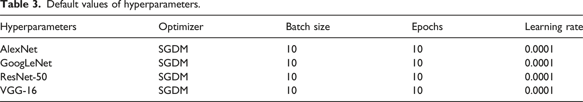
Air compressors are critical components in many industries whose catastrophic failure results in huge financial losses and downtime leading to accidents. Hence, real time fault diagnosis of air compressor is essential to predict the health condition of air compressor and plan scheduled maintenance thereby reducing financial losses and accidents. Fault diagnosis using transfer learning aids in real time fault detection. In the present study, five air compressor conditions were considered namely, check valve fault, inlet and outlet reed valve fluttering fault, inlet reed valve fluttering fault, outlet reed valve fluttering fault, and good condition. The raw vibration data was converted to radar plot images that were pre-processed and classified using four pre-trained networks (ResNet-50, GoogLeNet, AlexNet, and VGG-16). The hyperparameters like epochs, batch size, optimizer, train-test split ratio, and learning rate were varied to find out the best network for air compressor fault diagnosis. ResNet-50 among all other pre-trained networks produced the maximum classification accuracy (average of five trials) of 98.72%.

Keywords

Pre-trained models deep learning air compressor ResNet-50 GoogLeNet AlexNet and VGG-16

Introduction

Air compressors are devices that compress and store air by converting power, commonly sourced from a gasoline engine, diesel engine, or electric motor. Air compressors primarily store the potential energy in the form of compressed air by increasing the pressure of the air. This compressed air can be applied for multiple purposes, including operating industrial machinery, inflating tires, supplying air for HVAC systems and powering pneumatic tools. Numerous industries such as wood products, plastics, power generation, pharmaceuticals, glass manufacturing, mining, medical, food and beverage, general manufacturing, chemical manufacturing, electronics, aerospace, automotive, and many more have adopted the use of compressors. Air compressors can vary in size and type, from compact portable models to heavy-duty industrial versions. An air compressor that pressurizes and compresses air in one piston movement and then transfers it to a storage reservoir or other device is known as a single-stage, single-acting air compressor. The piston moves downwards in this process to pull air from the environment into the tank or system through the intake valve, then moves upwards to compress the air and send it out through the outlet valve.

Frequent observations state that mechanical apparatus is expected to experience wear and tear. The faults stem from various factors such as improper fittings, inappropriate working environment, corrosion, manufacturing defects, fatigue, external damage, electrical issues, overheating, contamination, improper sizing, and so on. Defects in the check valve, fluttering of the inlet reed valve, fluttering of the outlet reed valve, and fluttering of both the inlet and outlet reed valves are frequently noted faults in reciprocating air compressors used in industries. These faults can affect the reliability and performance of the air compressor and can also result in low output pressure, overheating, excessive vibration, oil leaks, excessive noise, and so on. According to research, 272 mishaps out of a total of 773 were caused by defective machinery. Thirteen of those mishaps caused immediate injury to people. An unintentional event occurs for about 68.8% of faults. Wear and strain on machines are unavoidable due to the constant and prolonged usage. Such scenarios may hinder the process and possibly lead to serious problems in commercial situations. Unexpected equipment failures can sometimes result in fatalities and even cause significant financial losses for businesses. Therefore, it is vital for industries to regularly monitor and diagnose machine faults to prevent such mishaps.

Manual methods of defect identification such as visual examination, sound tests, airflow tests, and pressure tests are undesirable or impractical for a variety of reasons. Manually defect detection is a sluggish and monotonous procedure that requires a high level of instrument knowledge and proficiency. Numerous fault identification techniques are available among which thermal imaging, oil analysis, vibration monitoring, and acoustic emission monitoring are frequently used in air compressors. Due to the fact that a sensor is not connected to the compressor, techniques that rely on thermal and acoustic data are referred to as non-invasive. The techniques widely adopted for fault diagnosis are briefly explained.

Oil analysis

To find possible issues in an air compressor, lubricant sampling is used. Using this method, a sample of the lubricant acquired from the compressor is examined for various contaminants such as metal fragments, water, and other substances that signify wear or harm to the internal components of the compressor. By determining the viscosity of the oil and lubricating properties, oil analysis can also aid in lubrication system optimization. However, oil analysis is difficult and complicated technique^1,2 that can yield inaccurate findings. Additionally, oil analysis can detect faults in components which come in contact with the oil and time-consuming as the sample should be taken to the laboratories to conduct the tests. As a result, real-time fault diagnosis may not be feasible, which could result in downtime.

Thermal imaging

Identification of air compressor faults can be aided by the use of thermal analysis. This is due to the fact that numerous faults in air compressors result in temperature fluctuations that can be monitored and studied using thermal imaging or other temperature-measuring equipment. Fault diagnosis using thermal imaging has numerous advantages like early detection, high resolution, non-invasive, comprehensive analysis, efficient, and quick. Even though thermal imaging has numerous advantages there are some potential disadvantages like interference, cost, skill, and training which make its use limited.^3,4

Acoustic based

The term acoustic analysis describes the use of sound data to pinpoint mechanical faults including those in air compressor. It entails identifying and classifying variations in sound patterns that are related to specific flaws or failures such as bearing wear, imbalance, or misalignment. The major advantages in using acoustic signal-based method for fault detection in air compressor are early detection, reduced downtime, elimination of catastrophic failure, non-invasive, cost-effective, and ease of data collection. The main disadvantage of this method is that external noise and unwanted sound signals may influence the results thereby affecting the accuracy, elevating the time and level of difficulty of pre-processing.^5–7

Vibration signal based

One common practice in identifying faults in mechanical systems is to analyze vibration signals. This method basically entails observing the vibrations that the system creates during operation. Faults can be identified when there is a change in the vibration signals produced. The intensity and type of faults depend on the produced vibration signals. Typically, moving components like bearings, gears, pistons and valves can malfunction in air compressors. These flaws may change the compressor vibration patterns that can be identified and assessed using signal processing methods and vibration monitors. The advantages of this method include cost-effectiveness, downtime reduction, and catastrophic breakdown limitation that aids in real time fault detection. Scheduled maintenance can be planned well in advance since comprehensive information about the faults including the severity and type of faults can be performed repeatedly over time. Vibration analysis is an invasive method and the optimal area for positioning the sensor must be found out to get the best and effective results.^8,9

After weighing the benefits and drawbacks of the available techniques, the vibration-based approach was selected as the preferred method for this investigation. Researchers frequently capitalized on machine learning techniques for classifying defects in vibration-based fault diagnosis. The literature provides significant results for creating a reliable and efficient fault diagnosis method which are described below. Golmoradi et al. conducted a study on the blades of a compressor to diagnose faults. A radial basis kernel function was equipped with support vector machines (SVM) to classify the extracted features and detect faults in blade of compressor.¹⁰ Tran et al. conducted a study that employed a hybrid deep belief network that combined Boltzmann machines and adaptive resonance theory map (ARTMAP) for the purpose of diagnosing air compressor faults. Statistical features were extracted from three signals: pressure, vibration, and current to diagnose faults.¹¹ An intelligent fault diagnosis study was performed by Liu et al., to detect four conditions of air compressor with the aid of stacked de-noising auto encoder (SDAE) and local mean decomposition (LMD).¹² Mohan and Sundaram conducted a study to diagnose faults in a compressor using different machine learning methods. They tested the compressor under seven different conditions and used principal component analysis (PCA) to extract features. To classify the faults, several techniques including k nearest neighbor (kNN), recursive partitioning and regression trees (RPART), C50, and SVM were used. The highest accuracy in classification was achieved by SVM with 97.25%.¹³ Prashanth and Elangovan used tree-based classifier family to classify the statistical features extracted from vibration signals acquired for various air compressor conditions to carry out fault diagnosis.¹⁴ Tang and Lin used adaptive waveform decomposition to diagnose multiple air compressor faults from vibrational signals.¹⁵ Machine learning techniques are now frequently used to spot faults in air compressors and perform classification. Tong et al. conducted a study on leakage faults in air compressors by analyzing infrared thermal images. Wavelet threshold algorithm (WTA) were used to pre-process the thermal images that were further improved with the help of firefly algorithm (FA). Otsu-Grab algorithm was used for image segmentation while histogram of oriented gradient (HOA) and gray level co-occurrence matrix (GLCM) were used majorly for calculating the features. SVM was used to classify the extracted features.¹⁶ An important aspect inside fault diagnosis is the concept of remaining useful life prediction which has been clearly explained in several works of literature involving multi hop cross pooling generative adversarial network¹⁷ and adaptive noise estimation & capacity regeneration.¹⁸ The following steps are followed to classify faults in machine learning process:

• Data collection: This is the first step in the machine learning process where the raw data is collected in the form of vibration, acoustic, speed, pressure, thermal image, current, and so on.

• Feature Extraction: The process of feature extraction entails taking significant and pertinent information out of raw data so that it can be used as input for a machine learning algorithm. Or, to put it another way, it involves choosing and transforming raw data into a set of features that can more effectively depict the data. This is done by using processes like wavelet transforms, principal component analysis, statistical feature extraction, Fourier spectral analysis, and many more.¹⁹

• Feature Selection: In this process, the features which play a vital role in determining the final accuracy are retained while those features that do not contribute much are excluded. This also helps in reducing the dimensionality of the data.¹⁴

• Classification: This is the final stage where the selected features are classified and faults are detected. This is done with the help of many classifiers like support vector machines,²⁰ miscellaneous classifiers, self-organizing maps,²¹ naïve Bayes,²² k-nearest neighbor,²³ decision trees,²⁴ etc.

Verma et al. evaluated various transformations that can be applied to vibration data to derive characteristics and determine the right transform for a given defect to improvise on the accuracy obtained.²⁵ Thus, from the above literature, it is evident that the features extracted play a crucial role in determining the final accuracy. However, the act of choosing the suitable method for extracting features for a specific issue demands a higher level of proficiency and understanding in the relevant field. Furthermore, manual feature selection has many disadvantages like labor-intensive, slow, and difficult.²⁶ Also, while extracting features manually, there is a high chance of rejecting good features that can improvise accuracy. Hence, manual feature selection is not a reliable fault diagnosis method. Therefore, there exists a high necessity to create an intelligent and efficient fault diagnosis method that can solve all the above said problems. A novel and effective solution to this problem is by deploying artificial intelligence through deep learning.

Deep learning refers to a specialized area of machine learning that employs artificial neural networks that contain numerous layers to comprehend and simulate intricate data patterns. In contrast to conventional machine learning techniques (that typically necessitate manually designed feature engineering), deep learning algorithms are capable of directly learning feature representations from the unprocessed input data. Deep learning algorithms are believed to serve as the building blocks in the upcoming industrial technology due to the boom in learning capabilities and potential applications.²⁷ Hinton and a team of researchers first introduced the idea of deep learning in 2006. Deep neural networks can yield excellent results in classification and regression-related problems when they are trained appropriately.²⁸ In machine learning, there is a significant fall in accuracy with the growing size of the dataset. Moreover, a high computational time is required to train the model if the size of the dataset is huge. However, these advantages are called off when deep learning is used since the accuracy of deep learning models increases with increase in the size of the dataset.²⁹ Machine learning and deep learning have some parallels in terms of pre-processing, model development, training, and categorization. The feature extraction procedure is not automated in machine learning, whereas it is in deep learning, which serves as great importance. The best features will be selected and as a result the classification accuracy will improve with reduced complexity thereby eradicating high level of domain expertise.³⁰ Thus, deep learning is more preferable for problems with huge number of datasets.³¹ The functioning of neural networks mimics that of the neurons present in the human brain, where connections between nodes in one layer are made with those in neighboring levels. The number of layers within the network determines its depth.

In this present study, fault diagnosis is done on single stage single acting air compressor using four different deep leaning networks namely, ResNet-50, GoogLeNet, AlexNet, and VGG-16. The networks are pre-trained and five hyperparameter namely, epochs, batch size, optimizer, train-test split ratio, and learning rate were varied to find out the best classification accuracy with the best hyperparameter selection. The following are the technical contributions made in this study:

• The study described in this article employs radar plots to display vibration signals in a clear and understandable manner. This technique is simpler than other image generation methods such as fast Fourier transforms and empirical mode decomposition, as it does not demand computer expertise or extensive mathematical knowledge.

• In this experimental work, various conditions that occur in air compressors such as check valve fault (PRV), inlet and outlet reed valve fluttering fault (IOVF), inlet reed valve fluttering fault (IVF), outlet reed valve fluttering fault (OVF), and good condition were considered.

• Transfer learning assisted classification was carried out using pre-trained deep learning networks such as ResNet-50, GoogLeNet, AlexNet, and VGG-16 due to the strong computational capabilities.

• To find the best setup for each pre-trained network, a series of experiments involving the modification of the hyperparameters such as epochs, batch size, optimizer, train-test split ratio, and learning rate were performed. The goal was to determine the optimal configuration for each network.

• Further, to eliminate randomness, five trails were run for each network with their optimal configuration and the best performing network was selected to diagnose faults in a single stage single acting air compressor.

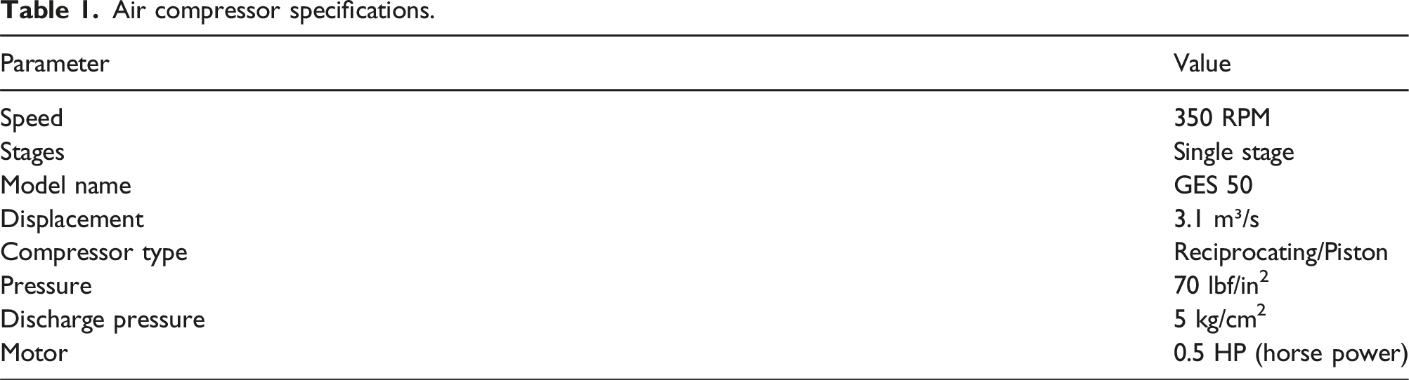
Experimental setup

The current study utilizes a single stage reciprocating air compressor whose specifications are as displayed in Table 1. The placement of accelerometer (sensor) was pre-determined for acquiring the vibration signals that necessitates a trustworthy data collection spot to make fault detection easier. The adhesive mounting technique was used to mount the accelerometer. In this study, vibration data were collected using a piezoelectric type accelerometer, the DYTRAN 3055 B1 model. This accelerometer weighs 10 g, has a 500 g working range, a sensitivity of 10 mV/g, a highest frequency response greater than 10 kHz and can operate between −15°C and 121°C. The accelerometer was mounted using adhesive in a vertical position over the piston head of the compressor to effectively collect signals. Furthermore, the sensor was linked to the NI-4432 DAQ system for better analog measurement. The fault circumstances for the research were created manually. The overall workflow is presented in Figure 1 while the adopted experimental setup is presented in Figure 2.

Table 1.

Air compressor specifications.

Parameter	Value
Speed	350 RPM
Stages	Single stage
Model name	GES 50
Displacement	3.1 m³/s
Compressor type	Reciprocating/Piston
Pressure	70 lbf/in²
Discharge pressure	5 kg/cm²
Motor	0.5 HP (horse power)

Figure 1.

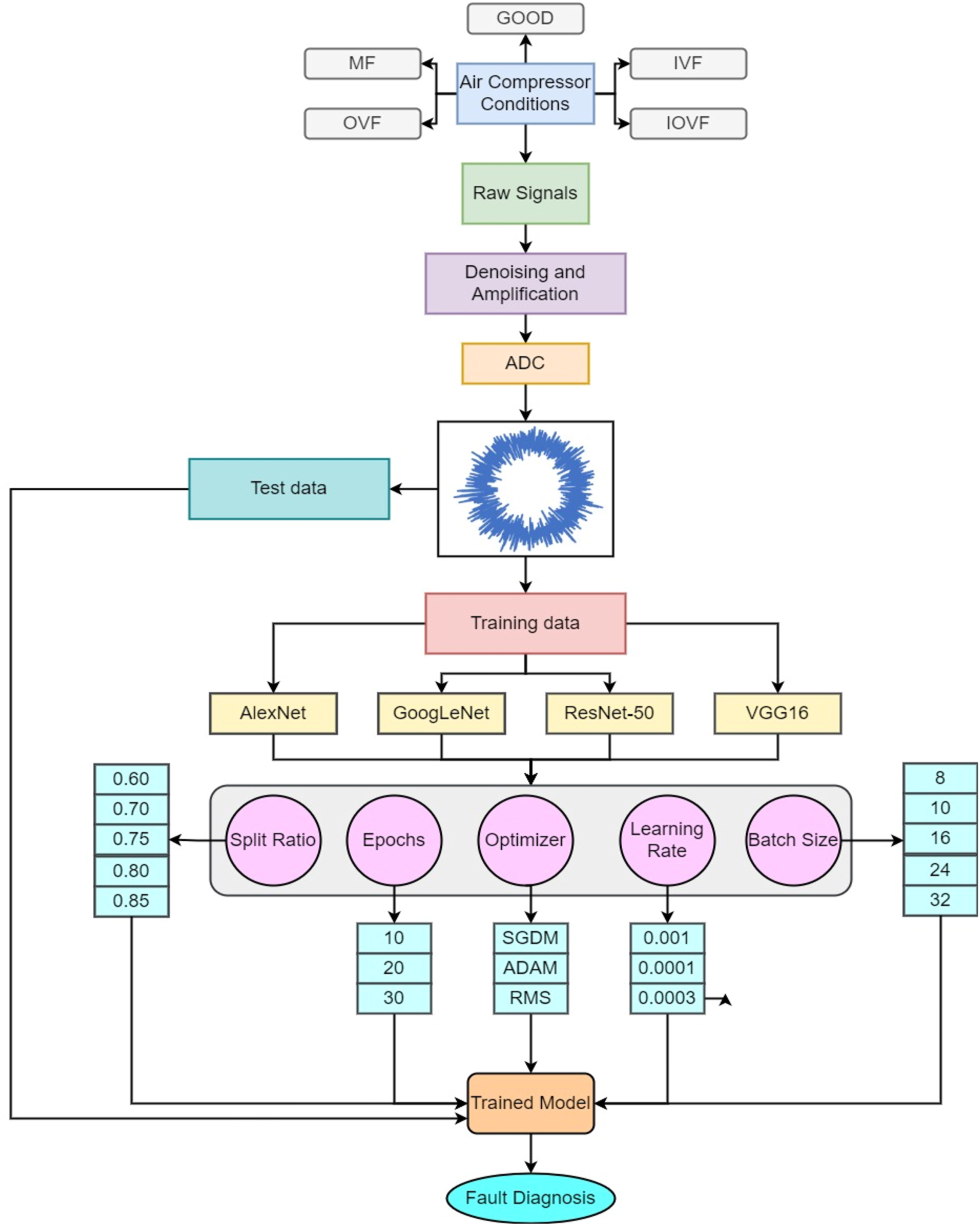
Overall methodology for fault diagnosis of air compressor.

Figure 2.

Experimental setup.

Data acquisition

The accelerometer sensor generates analog data which is then converted into digital format through the data acquisition (DAQ) system. This process enables the storage, analysis, and visualization of vibration signals. The analog signals are conditioned, processed, and digitalized by the Ni- 4432 DAQ setup via an USB chassis, with LabVIEW software being utilized for the entire process. The collection of signal involves consideration of various parameters. A sample representation of various signals collected is presented in Figure 3.

Figure 3.

Sample vibration signals of different air compressor conditions. (a) PRV (b) OVF (c) IVF (d) IOVF (e) GOOD.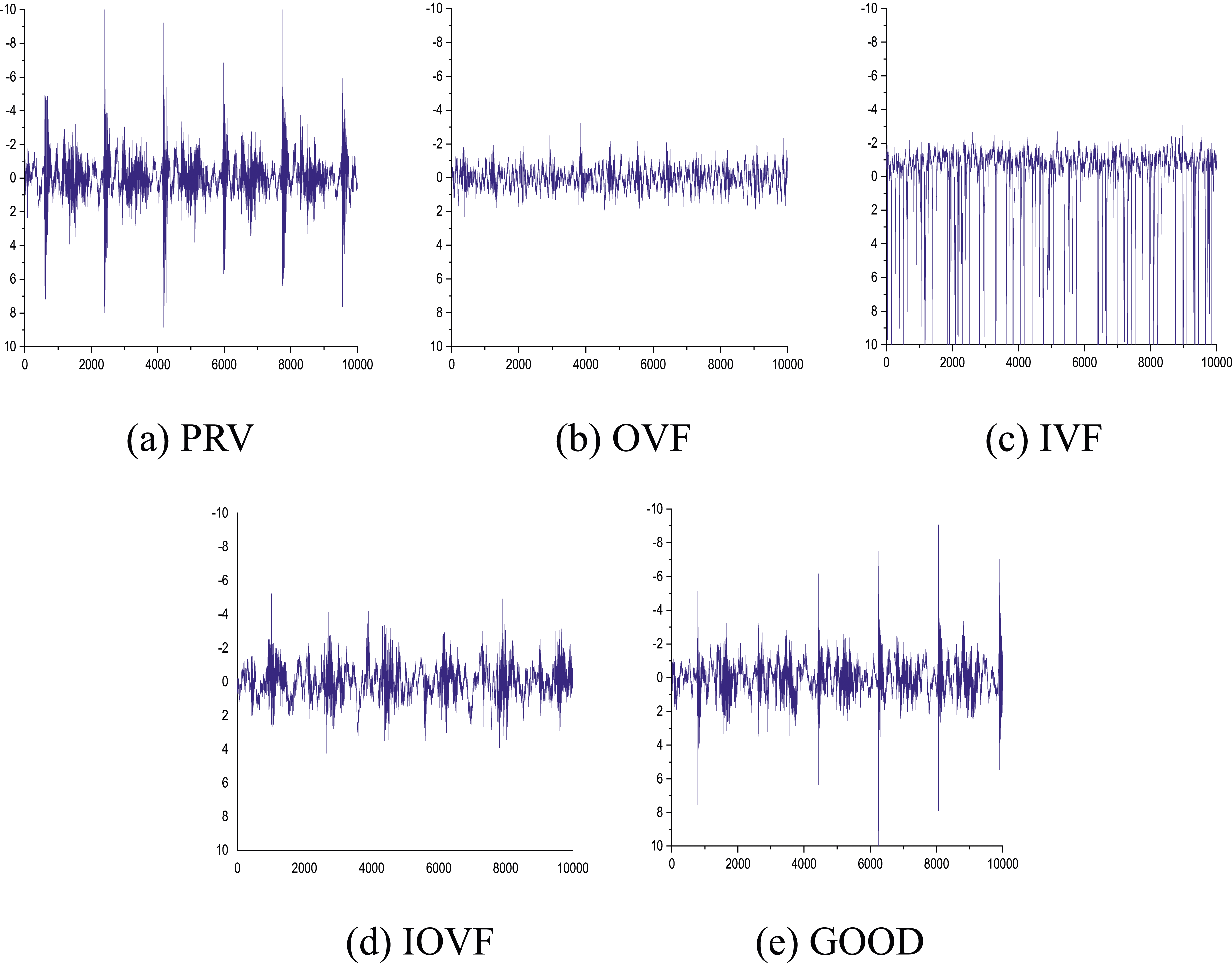

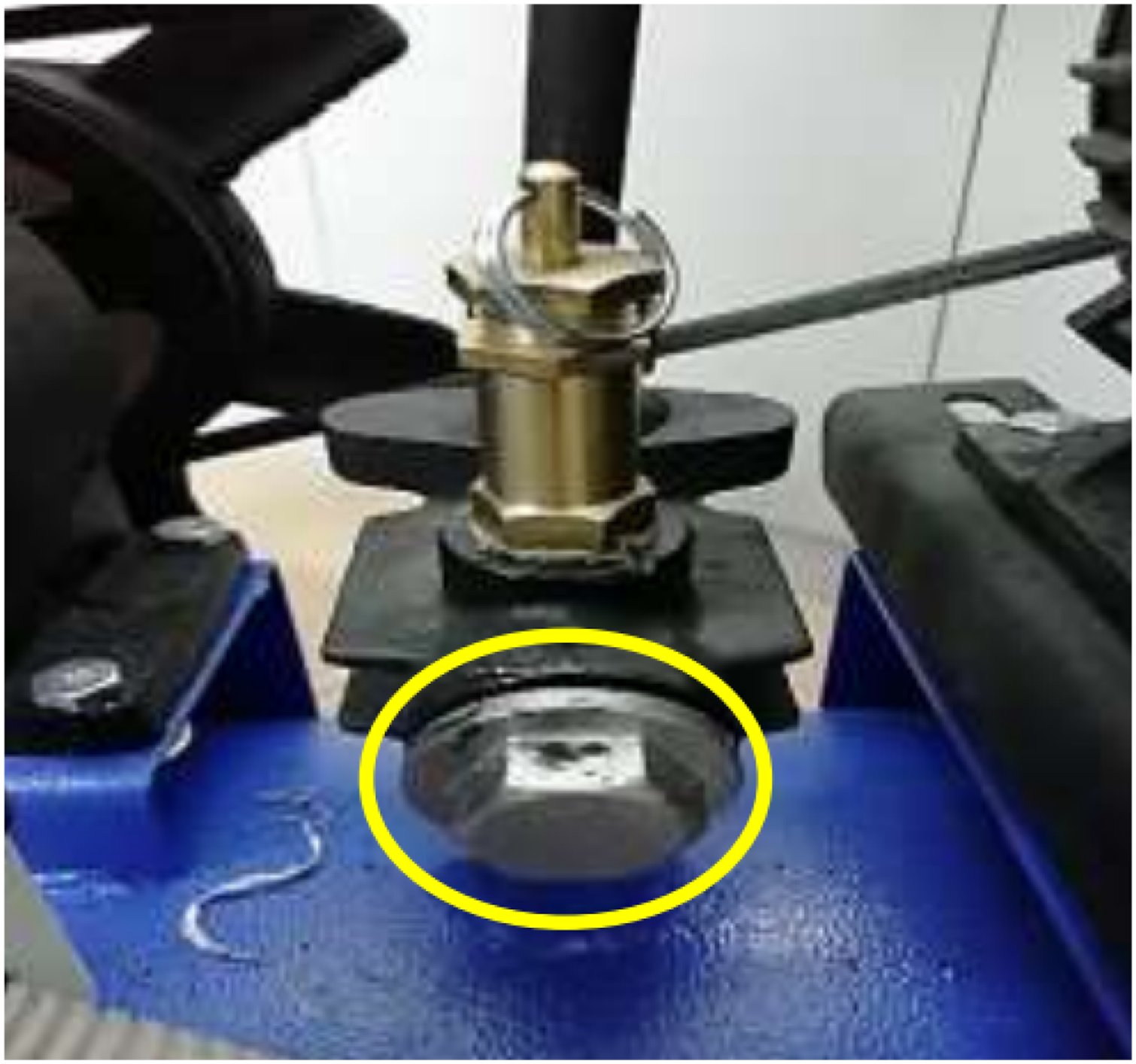
Faults in air compressor

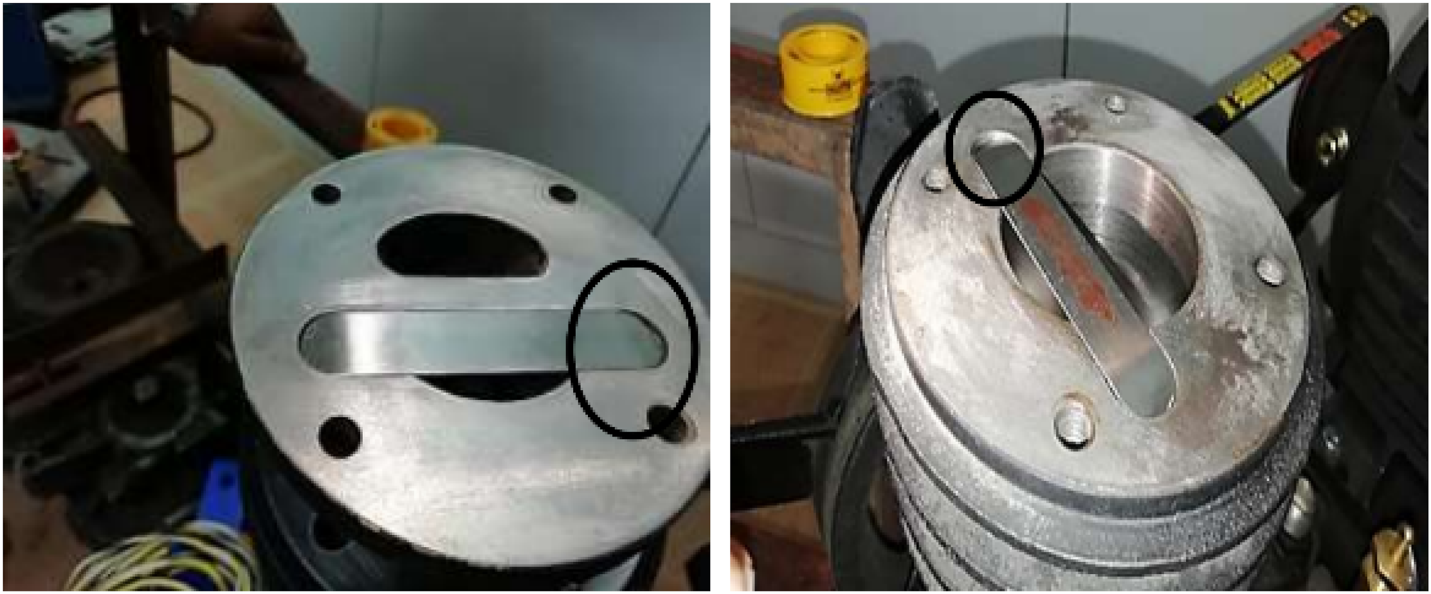
Due to wear and tear, air compressors are prone to a variety of inherent faults over time. The reliability, usefulness, and longevity of the system may be adversely impacted by these faults. Even though fault occurrences in machine components is a natural process, the faults considered in the study were intentionally reproduced for the purpose of research. There are five typical problems considered in the study that air compressors can experience.

1) Check valve fault: Check valve fault can be encountered when the valve arrangement has a leak and air particles exit as presented in Figure 4. Alternately, the issue can be directly reproduced by inserting a diaphragm material (broken) in the check valve configuration.

2) Inlet and outlet reed valves plate fluttering: When the inlet and exit valves do not sit properly, fluttering can happen. This is frequently brought on due to the rust development brought on by the existence of moisture in those valves. The reed valves can be inverted to achieve the fluttering action manually. Figure 5 represents the condition.

3) Outlet reed valve plate fluttering: If the outlet valve does not settle correctly, rust may develop due to moisture in the valve that can induce fluttering. The reed valves can be inverted to achieve the fluttering action manually.

4) Inlet reed valve fluttering: If the inlet valve does not settle correctly, rust may develop due to moisture in the valve that can induce fluttering. The reed valves can be inverted to achieve the fluttering action manually.

Figure 4.

Check valve fault.

Figure 5.

Inlet and outlet valve fluttering (Inverting valve plates upside down).

Description of convolutional neural network

A very powerful deep neural network for pattern recognition, image processing, and speech processing is the convolution neural network. Yann LeCun originally presented the idea in the 1980s. The fundamental tenet of CNN is that there is no spatial correlation between the features. The initial layer of the convolution neural network is the convolutional layer which is followed by subsequent convolutional layers, pooling layers and a fully connected (FC) layer at the very end. The complexity of the network rises with the number of layers. Using a hierarchical approach, the picture data is analyzed, starting with smaller aspects like colors and borders and working up to bigger ones like object forms. In a CNN, artificial neurons undertake mathematical operations to determine the weighted sum of multiple inputs and outputs of an activation value, similar to how biological neurons work. With an image as its input, a convolutional neural network creates several activation maps using different layers. Each input pixel patch is multiplied by weights, added together, and then the activation function is applied to it. The name convolutional network refers to the technique of convolution which involves adding the weights and pixel values together.

The difficult, yet crucial task is the process of training a neural network. By adjusting their weights, the neurons of the neural network are trained to recognize the proper characteristics in pictures. The weights of the neurons are initially adjusted at random, and the output is then compared with the appropriate label. The weights are slightly changed to reduce mistake if the output is inaccurate. Instead of randomly changing the units, the backpropagation approach is utilized to determine which neurons need to be altered in order to optimize this process. A whole cycle across the whole training dataset is referred to as epoch. The network becomes better at adjusting after each epoch, leading to a satisfactory fit ultimately. The network is tested using a different dataset that was not used during training once the training phase is complete. This will guarantee that the network can function well with fresh, untested data. In testing, similar to training, the output from the network is compared to the original label of the dataset. The network is said to be overfitted if it performs well during training but badly during testing. The network should be trained using a variety of datasets to avoid this problem. Convolutional neural network has a general architecture as represented in Figure 6.

Figure 6.

Fundamental structure of convolutional neural networks.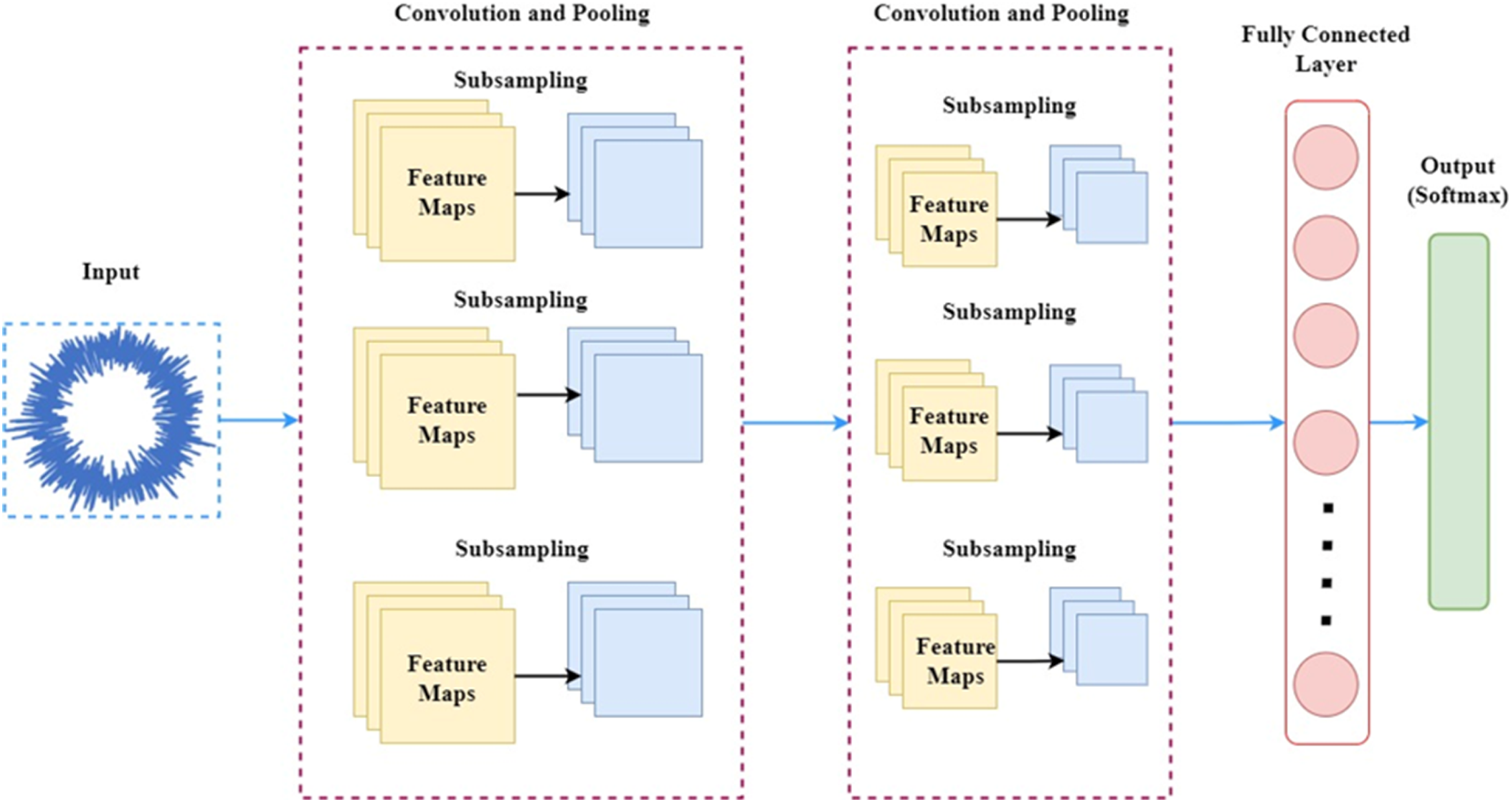

Convolutional layer

A convolution layer, which is composed of a group of parameterized learnable filters or kernels, is used throughout the learning process in CNN. These kernels are built to support a variety of inputs while being dispersed across a smaller area of space. For each picture input into the filter during convolution, two-dimensional activation maps are created. The scalar product of weights and volume is generated for each image data point that passes through the convolution gradient kernel. The network can recognize important properties in the spatial domain owing to the value each activation produces. Through tweaks to hyper-parameters like depth (number of filters), zero-padding (boundary of the input picture by enclosing it with zeros), and stride (filter movement in a single direction), the convolution layer may also lessen model complexity while improving performance.³² The mathematical operation performed in a convolution layer can be described in equation (1) wherein $a$ represents the input image, $b$ is the filter, and $\times$ represents the convolution operation

(a \times b) (t) = \sum_{τ = 0}^{T - 1} a (τ) . b (t - τ)

(1)

Furthermore, each convolution operation is accompanied by an activation function that introduces non-linearity into the model. Equation (2) represents the most commonly used activation function, rectified linear unit (ReLU). The presence of activation function helps in breaking the linearity among complex patterns such that the network can learn extensively

R e L U (z) = \max (0, z)

(2)

Pooling layer

The output from the convolution layer, such as its width and height, are reduced in spatial dimensions by the pooling layer of a CNN. It down samples each feature map in order to do these using methods like average pooling or maximum pooling. In addition to lowering the number of parameters in the network and preventing overfitting, this down sampling also strengthens the resistance of the network to input picture translations. Pooling can be done periodically or after each convolutional layer to further minimize the dimensionality. The down sampling results in smaller feature map sizes and faster training.³³ Equation (3) portrays the working of max pooling function wherein $P$ represents the pooled feature map, $s$ is the size of the pooling filter and $k$ is the input feature map

P_{a, b} = \max {k_{a + c, b + d}} for 0 \leq c, d < s

(3)

Fully connected layer

The output of final pooling layer is fed as input for fully connected layer which are some end layers of the network and are just uncomplicated feed-forward neural networks.³⁴ The fully connected layer aids in the connection of every neuron in one layer to the neurons in the next layer. The fully connected layer works on the operation expressed in equation (4) wherein $b$ is the output, $W$ is the weight matrix, $x$ is the bias vector, and $a$ is the input

b = W a + x

(4)

Fault diagnosis of air compressor using pre-trained models

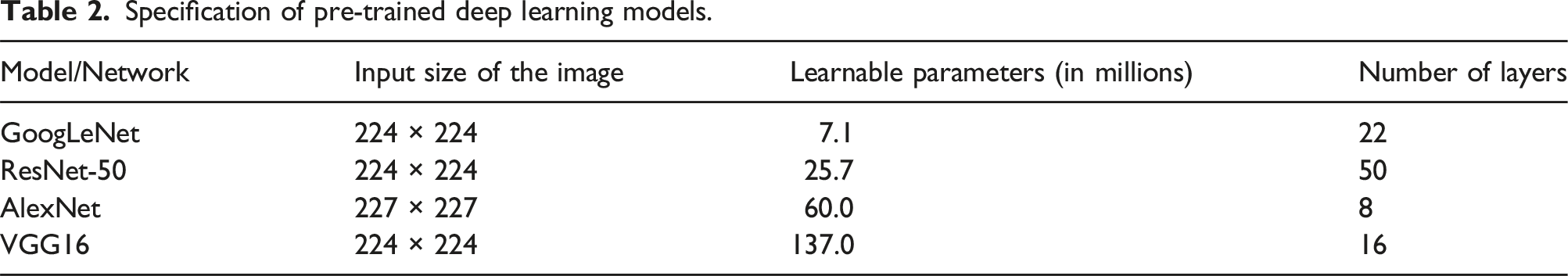
This section talks in detail about the methodology and process involved in air compressor fault diagnosis and also about the pre-trained models used. The present study uses the raw data acquired from the accelerometer and converts it in the form of radar plots. Radar plots are a graphical representation of data that represents every variable in the axis with same origin point. The variable values of every element are further plotted along the respective axis in a series of point resulting in a polygonal shaped plot. Radar plots are preferred in the current study due to the following advantages: (i) multiple dimensional data visualization, (ii) easy interpretation, (iii) comparable, (iv) simple display of complex data, (iv) unique pattern, and (v) flexible nature. The acquired radar images were pre-processed and converted into two image sizes of 227 × 227 and 224 × 224 pixels, to feed the pre-trained network as per their image input size requirements. Then the images were fed into four pre-trained networks namely ResNet-50, GoogLeNet, AlexNet, and VGG-16, after which image classification was done to detect faults in air compressor. The hyperparameters like epochs, batch size, optimizer, train-test split ratio, and learning rate were varied to find the best value of each hyperparameter for each network, so as to achieve the highest possible classification accuracy. The whole workflow of air compressor fault classification using pre-trained networks is depicted in Figure 7. Table 2 describes a quick overview of the pre-trained models specifications used in the study.

Figure 7.

Overall workflow of air compressor fault classification using pre-trained networks.

Table 2.

Specification of pre-trained deep learning models.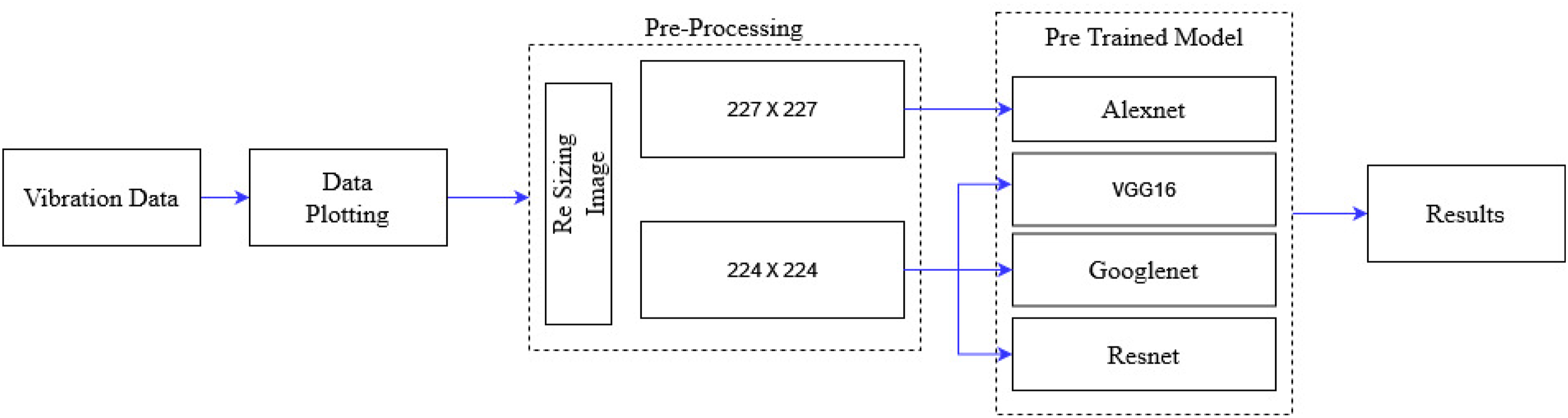

Model/Network	Input size of the image	Learnable parameters (in millions)	Number of layers
GoogLeNet	224 × 224	7.1	22
ResNet-50	224 × 224	25.7	50
AlexNet	227 × 227	60.0	8
VGG16	224 × 224	137.0	16

Dataset creation and pre-processing

The vibration signals were obtained for four defective conditions namely, check valve fault, inlet and outlet reed valve fluttering fault, inlet reed valve fluttering fault, outlet reed valve fluttering fault, and good condition. The acquired raw vibration signals were converted into radar plots with the help of Microsoft EXCEL. For each compressor condition, 75 radar plot images were obtained accounting to a total of 375 images. The radar plot images were pre-processed and resized to 227 × 227 and 224 × 224 pixels using MATLAB such that the images were in acceptable sizes for the pre-trained network. A sample of the radar plots depicting all condition of air compressor is shown in Figure 8.

Figure 8.

Vibration plots of various air compressor conditions. (a) Inlet and outlet reed valve fluttering fault. (b) Good condition. (c) Inlet reed valve fluttering fault. (d) Outlet reed valve fluttering fault. (e) Check valve fault.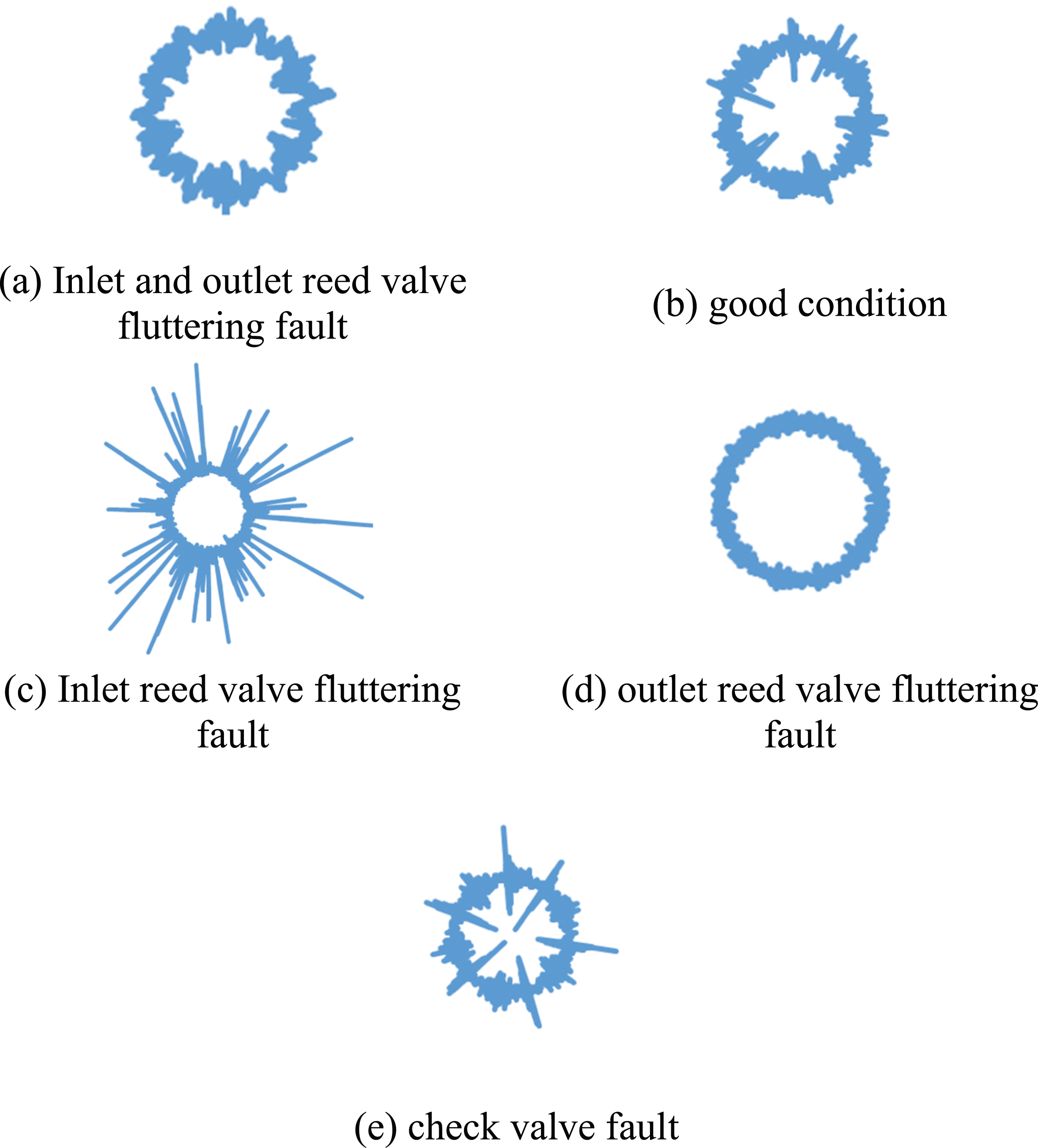

AlexNet

AlexNet, created by Alex Krizhevsky, is an eight-layer convolutional neural network comprising five convolutional layers, two fully connected layers, and one output layer. It became well-known during the ImageNet Challenge, featuring 61 million parameters and trained on 1.2 million images. The network employs ReLU activation, dropout layers, and data augmentation techniques. It processes images with dimensions of 227 × 227 pixels, reducing them to 13 × 13 pixels, and then uses fully connected layers and a softmax layer for classification, harnessing GPUs for enhanced efficiency.³⁵

ResNet pre-trained network

ResNet, introduced by Kaiming He and colleagues in 2015, tackles the vanishing gradient problem with its deep architecture, achieving first place in ILSVRC-2015 with a 3.75% error rate. Initially trained on the COCO dataset, ResNet’s architecture comprises stacks of residual units, along with convolutional, pooling, and fully connected layers. Being eight times deeper than VGG, it is capable of learning more features.

GoogLeNet pre-trained network

GoogLeNet, introduced by Szegedy et al. in the paper “Going Deeper with Convolutions,” achieves a lower error rate than both AlexNet and VGG. Its 22-layer architecture employs 1 × 1 convolutions and global average pooling for computational efficiency. The network includes nine inception modules, linked by convolutions, max-pooling, average pooling, fully connected layers, and softmax layers, effectively reducing image size while maintaining spatial information.³⁶

VGG-16 pre-trained network

VGG-16, developed by Karen Simonyan and Andrew Zisserman in 2014, was a leading performer in ILSVRC-2014. Unlike AlexNet, VGG-16 uses multiple 3 × 3 filters instead of single large filters. It consists of 13 convolutional layers, 3 fully connected layers, 5 max-pooling layers, and a final classification layer. VGG-16 processes 224 × 224 RGB images, with mean RGB values subtracted during preprocessing. Despite its depth and non-linearities, VGG-16 suffers from slow training speed and significant weight sizes.³⁷

Result and discussion

The vibration signals were obtained using an accelerometer and the raw data was converted into vibration plots. A total of 375 images were obtained, 75 images for one air compressor condition (check valve fault, inlet and outlet reed valve fluttering fault, inlet reed valve fluttering fault, outlet reed valve fluttering fault, and good condition). Four pre-trained networks namely, ResNet-50, GoogLeNet, AlexNet, and VGG-16 were deployed. The hyperparameters such as epochs, batch size, optimizer, train-test split ratio and learning rate were varied to find the best values of hyperparameters for each network, in order to obtain the highest classification accuracy possible. AlexNet was fed with input image of size 227 × 227 pixels while the other three networks were fed with image size of 224 × 224 pixels.

Effect of training – test ratio

From the total dataset, a specific percentage is dedicated to train the model and the other part of the dataset called the test dataset is used to assess the predictions of the trained model. For example, if a train-test ratio of 0.70 was assigned, 70% of the data will be used for training and 30% for testing. 0.60, 0.70, 0.75, 0.80, and 0.85 were the five train-test ratios that were varied in this experiment. The ratio that delivered the highest classification accuracy was fixed for each network. The default values were set for the other hyperparameters which is depicted in Table 3. The classification accuracies for various train – test split ratio is depicted in Table 4.

Table 3.

Default values of hyperparameters.

Hyperparameters	Optimizer	Batch size	Epochs	Learning rate
AlexNet	SGDM	10	10	0.0001
GoogLeNet	SGDM	10	10	0.0001
ResNet-50	SGDM	10	10	0.0001
VGG-16	SGDM	10	10	0.0001

Table 4.

Classification accuracies for various train-test split ratio.

Train test ratio	AlexNet (%)	GoogLeNet (%)	ResNet-50 (%)	VGG-16 (%)
0.60	97.3	94.0	96.7	98.7
0.70	97.3	96.4	97.3	96.4
0.75	98.9	96.8	100.0	98.9
0.80	98.7	97.3	97.3	97.3
0.85	100.0	92.7	98.2	96.4

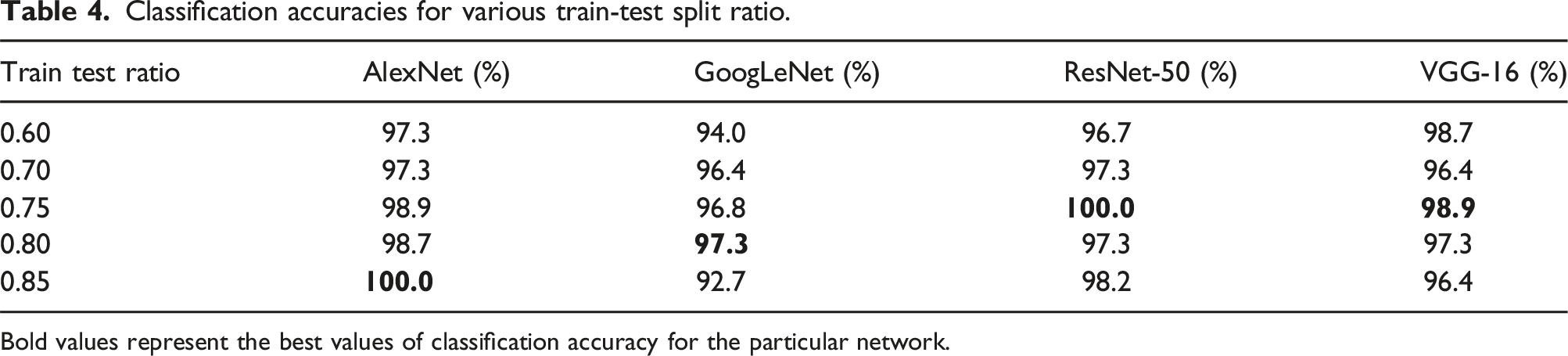
Bold values represent the best values of classification accuracy for the particular network.

Effect of optimizers

An algorithm or function known as an optimizer can change parameters like learning rate and weights to enhance the effectiveness of classification while minimizing total loss. Experiments were carried out employing optimizers such root mean squared propagation (RMSPROP), adaptive moment estimation (ADAM) and stochastic gradient descent (SGDM) to gauge the model performance in fault classification. The train-test ratio which gave the best classification accuracy (section 5.1) was fixed. For instance, the train test ratio for ResNet-50, GoogLeNet, AlexNet, and VGG-16 were fixed as 0.75, 0.80, 0.85, and 0.75, respectively. Further the optimizers were varied, fixing batch size, epochs and learning rate to their default values. The respective optimizer and their classification accuracy is depicted in the below Table 5.

Table 5.

Classification accuracies for various optimizers.

Optimizer	AlexNet (%)	GoogLeNet (%)	ResNet-50 (%)	VGG-16 (%)
SGDM	98.2	97.3	98.9	97.9
ADAM	92.7	98.7	83.2	94.7
RMSPROP	90.9	97.3	95.8	56.8

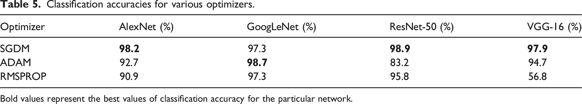
Bold values represent the best values of classification accuracy for the particular network.

Effect of batch size

The batch size refers to the size or number of samples used for training the dataset for each iteration. An increased batch size will result in more space consumption since a greater number of samples were used per iteration. In this study, five batch sizes namely 8, 10, 16, 24, and 32 were considered. The best performing optimizer and train-test ratio with highest efficiency for each network was fixed. For ResNet-50, AlexNet, and VGG-16 the optimizers were fixed as SGDM while GoogLeNet adopted ADAM. The epochs and learning rate were set to default values and the batch sizes were varied. The results obtained are depicted in Table 6.

Table 6.

Classification accuracies for various batch size.

Batch size	AlexNet (%)	GoogLeNet (%)	ResNet-50 (%)	VGG-16 (%)
8	98.2	94.7	97.9	96.8
10	100.0	94.7	97.9	96.8
16	98.2	97.3	98.9	92.6
24	100.0	100.0	96.8	98.9
32	100.0	96.0	94.7	94.7

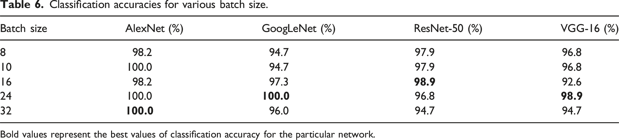
Bold values represent the best values of classification accuracy for the particular network.

Effect of epochs

The number of epochs signify the number of times the learning algorithm runs over the dataset dedicated for training. In this study, various values of epochs such as 10, 20, and 30 were considered. The learning rate was set to default and the values of train test ratio and optimizer was fixed to their optimal value from the previous sections. The batch size 24 for VGG-16 and GoogLeNet gave the highest classification accuracy while for ResNet-50 and AlexNet a batch size of 16 and 32, respectively, gave the best classification accuracy. Three batch sizes were fixed for their respective network and their epochs were varied. The classification accuracy was found and is depicted in Table 7.

Table 7.

Classification accuracies for various epochs.

Epochs	AlexNet (%)	GoogLeNet (%)	ResNet-50 (%)	VGG-16 (%)
10	94.5	97.3	98.9	98.9
20	98.2	97.3	97.9	96.8
30	100.0	98.7	97.9	100.0

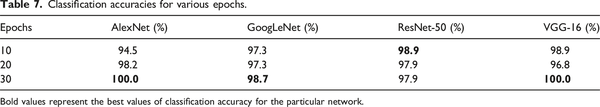
Bold values represent the best values of classification accuracy for the particular network.

Effect of learning rate

The learning rate is a critical factor in determining the accuracy as it the pace at which a model learns/adapts to a challenge. The learning rates considered in the study are 0.0001, 0.0003, and 0.001. The train-test ratio, epochs, batch size, and optimizers were fixed to their optimal values form the previous results. The epoch of 30 was found to be the best for AlexNet, VGG-16, and GoogLeNet and ResNet-50 had the best classification accuracy for a epochs of 10. These values were fixed and the learning rate was varied, whose results are depicted in Table 8.

Table 8.

Classification accuracies for various learning rate.

Learning rate	AlexNet (%)	GoogLeNet (%)	ResNet-50 (%)	VGG-16 (%)
0.0003	98.2	97.3	96.8	96.8
0.0001	100.0	100.0	95.8	100.0
0.001	92.7	86.7	98.9	98.9

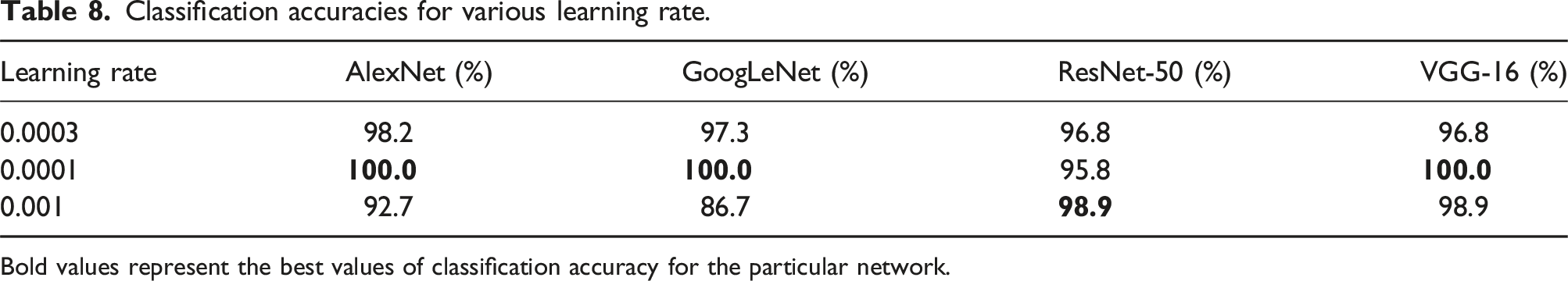
Bold values represent the best values of classification accuracy for the particular network.

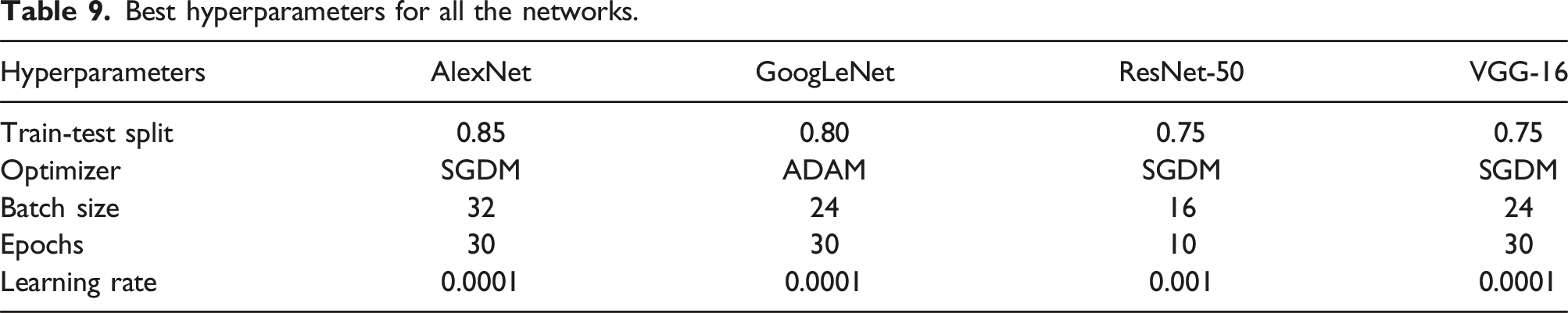
The best hyperparameters for all the networks were fixed, which is depicted in Table 9. Further these values were utilized for every network and run for five trails. To determine the efficient network, highest classification accuracy is considered as the evaluation criterion. The mean of five trails were taken and the network giving the highest classification accuracy was chosen to be the best which is depicted in Table 10. The trial runs were carried out in the present study to eliminate the randomness issue. Also, the trials were performed to eliminate the black box result projection. Table 10 shows the results for the five trials. From the above trials the best performing network was found to be ResNet-50 with a mean classification accuracy of 98.72% of all the four networks. Classification accuracy of 100.0% was the most frequent and highest classification accuracy for ResNet-50 that has occurred three out of the five trials. Hence, the confusion matrix and training progress for the most frequent classification accuracy is shown in Figures 9 and 10. Furthermore, the visualization of the image through every layer of ResNet-50 is presented in Figure 11. From Figure 11, one can understand how simple and complex features of an image are learned by a network. The figure represents 49 layers of visualization before being classified.

Table 9.

Best hyperparameters for all the networks.

Hyperparameters	AlexNet	GoogLeNet	ResNet-50	VGG-16
Train-test split	0.85	0.80	0.75	0.75
Optimizer	SGDM	ADAM	SGDM	SGDM
Batch size	32	24	16	24
Epochs	30	30	10	30
Learning rate	0.0001	0.0001	0.001	0.0001

Table 10.

Classification accuracy for five trails with best hyperparameters.

Trails	AlexNet (%)	GoogLeNet (%)	ResNet-50 (%)	VGG-16 (%)
1	98.2	98.7	96.8	98.9
2	98.2	97.3	100.0	100.0
3	96.4	96.0	100.0	96.8
4	89.1	97.3	100.0	96.8
5	98.2	97.3	96.8	97.9
Mean	96.02	97.32	98.72	98.08

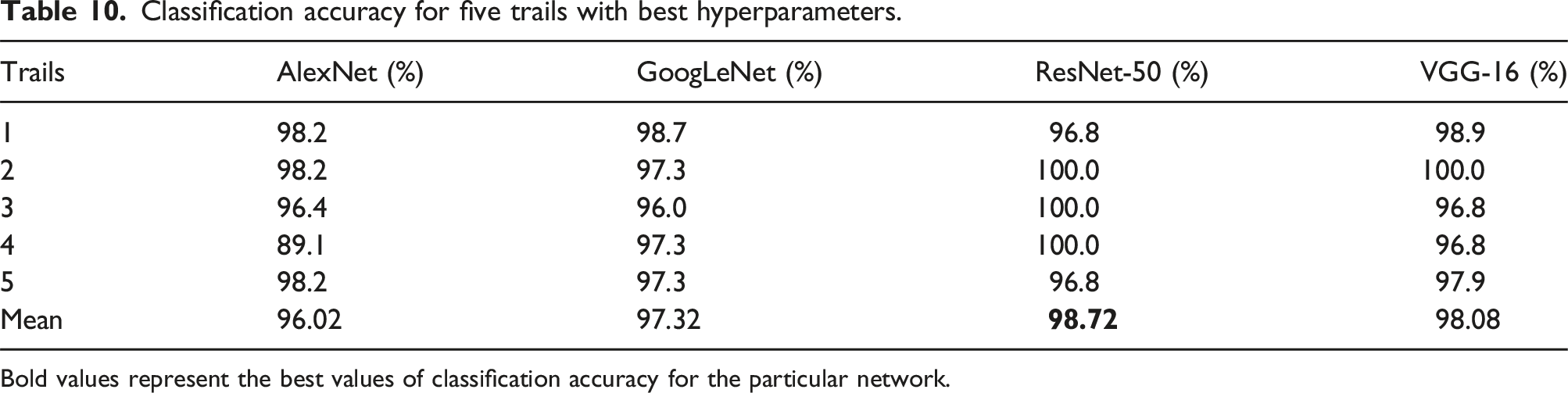
Bold values represent the best values of classification accuracy for the particular network.

Figure 9.

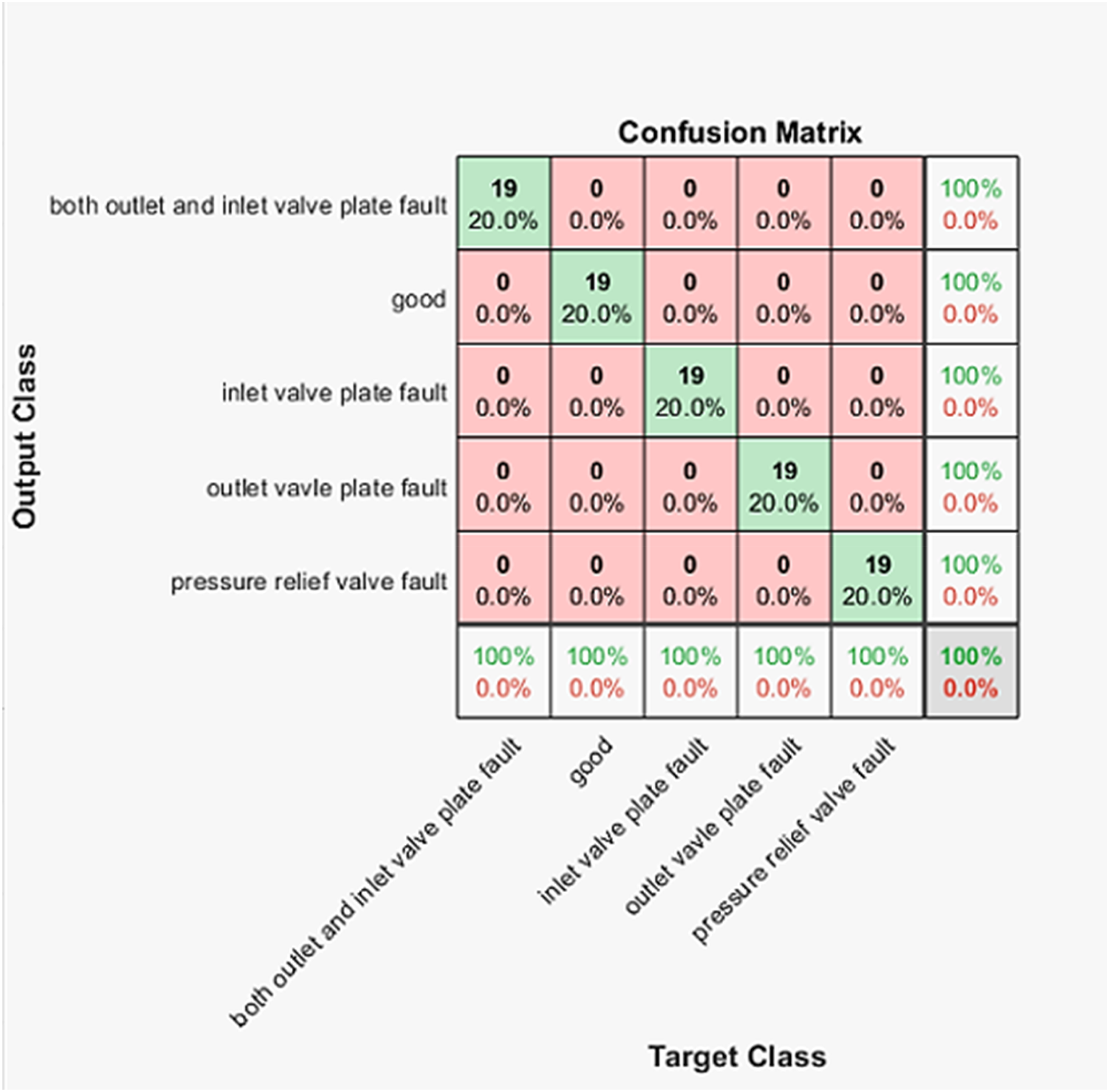
Confusion matrix of highest classification accuracy achieved in ResNet-50.

Figure 10.

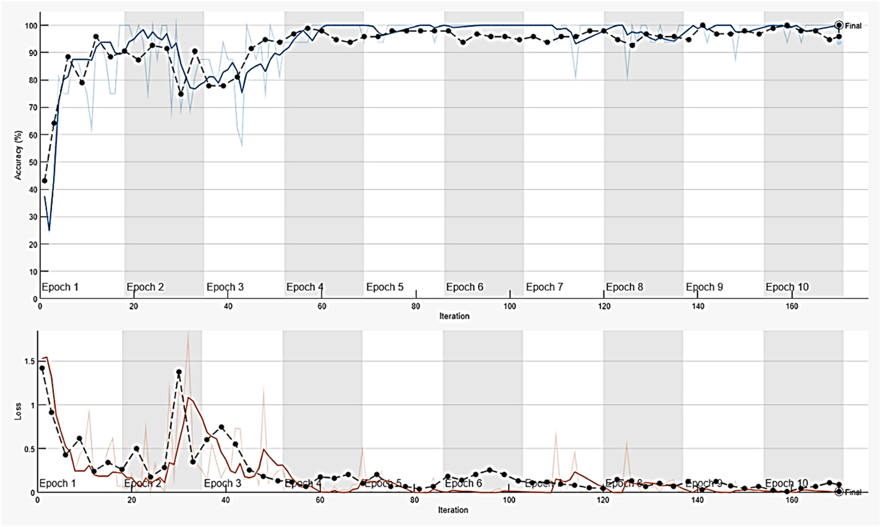
Training progress of highest classification accuracy achieved in ResNet-50.

Figure 11.

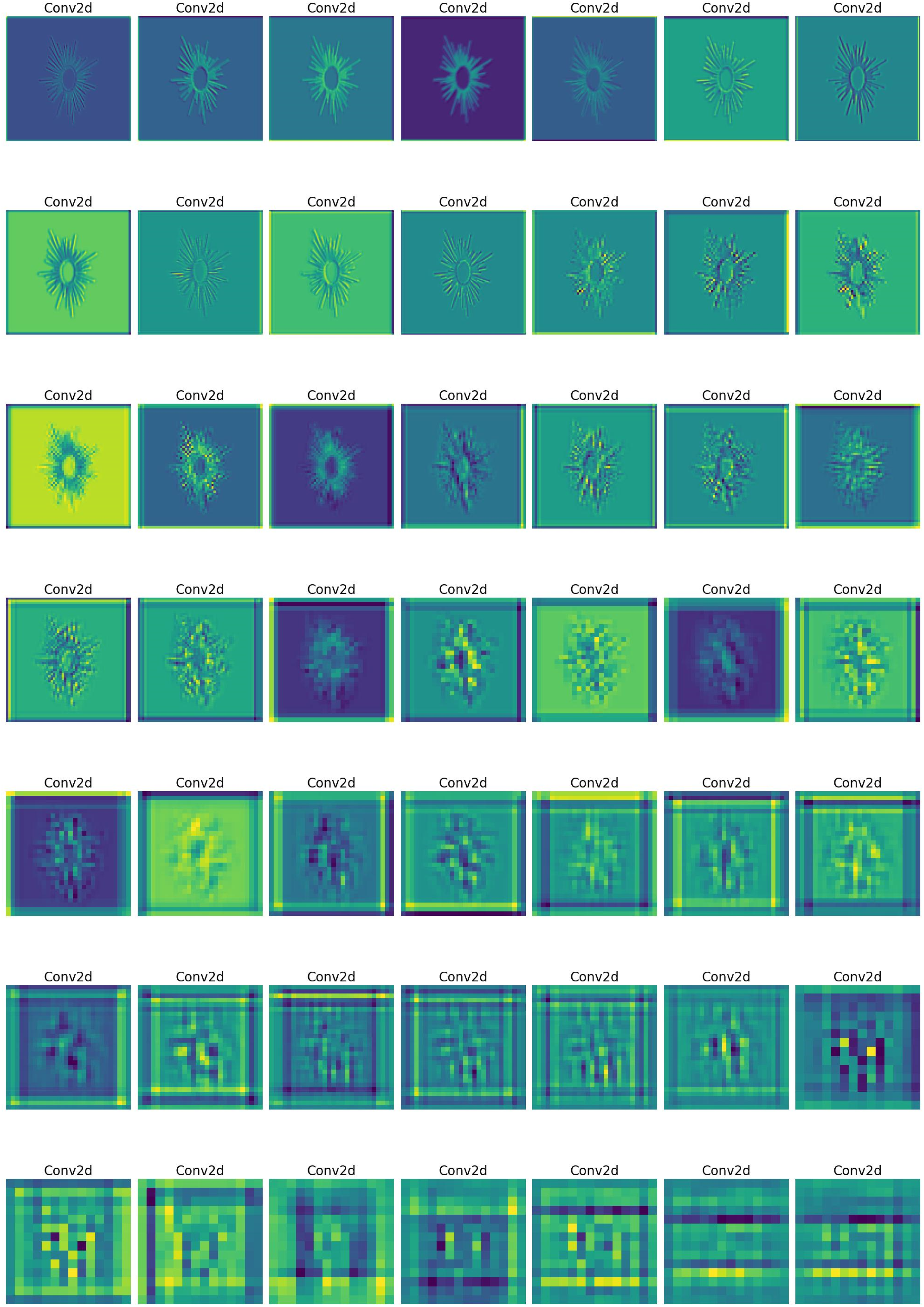
Visualization of ResNet-50 layers for inlet valve fault.

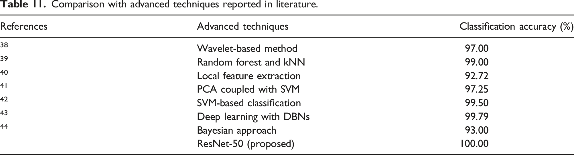
To establish the effectiveness of the proposed method, several state of the art techniques were compared in the present study as presented in Table 11.

Table 11.

Comparison with advanced techniques reported in literature.

References	Advanced techniques	Classification accuracy (%)
³⁸	Wavelet-based method	97.00
³⁹	Random forest and kNN	99.00
⁴⁰	Local feature extraction	92.72
⁴¹	PCA coupled with SVM	97.25
⁴²	SVM-based classification	99.50
⁴³	Deep learning with DBNs	99.79
⁴⁴	Bayesian approach	93.00
	ResNet-50 (proposed)	100.00

Conclusion

In this study, the efficacy of four pre-trained networks namely, ResNet-50, GoogLeNet, AlexNet, and VGG-16 were investigated for real-time fault detection in air compressors. Five distinct conditions of the air compressor were considered including check valve fault, inlet and outlet reed valve fluttering faults, inlet reed valve fluttering fault, outlet reed valve fluttering fault, and a healthy, operational state. To transform raw vibration signals into a suitable format for analysis, radar plot images were employed, resulting in a dataset comprising 375 images (75 images per condition). To optimize the performance of each pre-trained network, the hyperparameters such as epochs, batch size, optimizer, train-test split ratio, and learning rate were systematically varied. By identifying the most effective combination of hyperparameter values, five trials for each network were conducted to obtain a reliable estimate of classification accuracy. The findings revealed that ResNet-50 achieved the highest classification accuracy of 98.72%, making it the most suitable network for air compressor fault diagnosis among the models tested. Looking ahead, the prospect of on-board fault diagnosis holds significant promise as a practical technique for real-world applications. The availability of numerous pre-trained network models in open repositories offers ample opportunities for leveraging advanced machine learning capabilities in fault detection systems. Furthermore, the integration of micro-electromechanical systems (MEMS) sensors presents a potential avenue for enhancing the development of next-generation compressor diagnostics, potentially reducing sensor costs and facilitating broader implementation. In conclusion, the study underscores the importance of leveraging state-of-the-art machine learning techniques such as transfer learning with pre-trained networks for effective fault diagnosis in air compressors. By optimizing hyperparameters and exploring novel data representation methods, the study contributes to advancing the field of condition monitoring and predictive maintenance, ultimately striving towards safer and more efficient industrial operations.

Footnotes

Declaration of conflicting interests

The author(s) declared no potential conflicts of interest with respect to the research, authorship, and/or publication of this article.

Funding

The author(s) received no financial support for the research, authorship, and/or publication of this article.

ORCID iDs

V Sugumaran

Joshuva Arockia Dhanraj

Jenoris Muthiya Solomon

Data availability statement

The datasets generated and/or analyzed during the current study are available from the corresponding author on reasonable request.*

References

Pradhan

Mishra

. Analysis of ISO VG 68 bearing oil for condition monitoring collected from an externally pressurized ball bearing system. Mater Today Proc 2021; 44: 4602–4606.

Zhu

Erqinhu

, et al. Fault-diagnosis for reciprocating compressors using big data and machine learning. Simulat Model Pract Theor 2018; 80: 104–127.

Wan

, et al. Rotating machinery fault diagnosis based on convolutional neural network and infrared thermal imaging. Chin J Aeronaut 2020; 33: 427–438.

Zhiyi

Haidong

Xiang

, et al. An intelligent fault diagnosis method for rotor-bearing system using small labeled infrared thermal images and enhanced CNN transferred from CAE. Adv Eng Inf 2020; 46: 101150.

Liu

Pei

Lodewijks

, et al. Acoustic signal based fault detection on belt conveyor idlers using machine learning. Adv Powder Technol 2020; 31: 2689–2698.

Verellen

Verbelen

Stockman

, et al. Beamforming applied to ultrasound analysis in detection of bearing defects. Sensors 2021; 21: 6803.

Verma

Sevakula

Dixit

, et al. Intelligent condition based monitoring using acoustic signals for air compressors. IEEE Trans Reliab 2016; 65: 291–309.

Liang

Cao

Tang

. Rolling bearing fault diagnosis based on feature fusion with parallel convolutional neural network. Int J Adv Manuf Technol 2021; 112: 819–831.

Praveenkumar

Saimurugan

Krishnakumar

, et al. Fault diagnosis of automobile gearbox based on machine learning techniques. Procedia Eng 2014; 97: 2092–2098.

10.

Golmoradi

Ebrahimi

Javidan

. Compressor fault diagnosis based on SVM and GA. Vibroengineering PROCEDIA 2017; 12: 49–53.

11.

Tran

AlThobiani

Tinga

, et al. Single and combined fault diagnosis of reciprocating compressor valves using a hybrid deep belief network. Proc Inst Mech Eng C J Mech Eng Sci 2018; 232: 3767–3780.

12.

Liu

Duan

Yuan

, et al. An intelligent fault diagnosis method for reciprocating compressors based on LMD and SDAE. Sensors 2019; 19: 1041.

13.

Mohan

. AN analysis of air compressor fault diagnosis using machine learning technique. JOURNAL OF Mechanics of Continua and Mathematical Sciences. 2019; 14. doi:10.26782/JMCMS.2019.12.00002.

14.

R Ozdemir

Hacioglu

Kasapoglu

, et al. Vibration based fault monitoring of a compressor using tree-based algorithms. IOP Conf Ser Mater Sci Eng 2019; 577: 012116.

15.

Tang

Lin

. Fault feature extraction of reciprocating compressor based on adaptive waveform decomposition and Lempel-Ziv complexity. IEEE Access 2019; 7: 82522–82531.

16.

Tong

Wang

, et al. A novel Pipeline leak recognition method of mine air compressor based on infrared thermal image using IFA and SVM. Appl Sci 2020; 10: 5991.

17.

Zhang

Tian

Yan

, et al. Multi-hop graph pooling adversarial network for cross-domain remaining useful life prediction: a distributed federated learning perspective. Reliab Eng Syst; Saf;: 244. doi:10.1016/j.ress.2024.109950.

18.

Zhang

Jiang

, et al. Remaining useful life prediction of lithium-ion battery with adaptive noise estimation and capacity regeneration detection. IEEE ASME Trans Mechatron. 28. doi:10.1109/TMECH.2022.3202642.

19.

Abdelfattah

Ibrahim

. Health monitoring of automotive suspension system using machine learning. In: Proceedings of the 7th International Conference on Vehicle Technology and Intelligent Transport Systems - VEHITS. SciTePress, 2021, pp. 325–332.

20.

Sharma

Patel

Acharya

. Automated detection of abnormal EEG signals using localized wavelet filter banks. Pattern Recogn Lett 2020; 133: 188–194.

21.

Zhong

Yuan

, et al. Bearing fault diagnosis using transfer learning and self-attention ensemble lightweight convolutional neural network. Neurocomputing 2022; 501: 765–777.

22.

Glowacz

Tadeusiewicz

Legutko

, et al. Fault diagnosis of angle grinders and electric impact drills using acoustic signals. Appl Acoust 2021; 179: 108070.

23.

Mehta

Goyal

Choudhary

et al. Machine learning-based fault diagnosis of self-aligning bearings for rotating machinery using infrared thermography. Math Probl Eng 2021. DOI: 10.1155/2021/9947300, Epub ahead of print 2021.

24.

Joshuva

Sivakumar

Sathishkumar

Deenadayalan

Vishnuvardhan

. Fault diagnosis of wind turbine blades using histogram features through nested dichotomy classifiers. Int J Recent Technol Eng. 2019; 8(2): 193–201.

25.

Verma

Gupta

Sevakula

et al. Signal transforms for feature extraction from vibration signal for air compressor monitoring. In: IEEE region 10 annual international conference, proceedings/TENCON, Bangkok, Thailand, 26 January 2015. DOI: 10.1109/TENCON.2014.7022275.

26.

Tran

Althobiani

Ball

. An approach to fault diagnosis of reciprocating compressor valves using Teager–Kaiser energy operator and deep belief networks. Expert Syst Appl 2014; 41: 4113–4122.

27.

Sarker

. Deep learning: a comprehensive overview on techniques, taxonomy, applications and research directions. SN Comput Sci 2021; 2: 1–20.

28.

Kim

Cho

. Zero-day malware detection using transferred generative adversarial networks based on deep autoencoders. Inf Sci 2018; 460: 83–102.

29.

Xin

Kong

Liu

, et al. Machine learning and deep learning methods for cybersecurity. IEEE Access 2018; 6: 35365–35381.

30.

Sarker

Abushark

Alsolami

, et al. IntruDTree: a machine learning based cyber security intrusion detection model. Symmetry 2020; 12: 754.

31.

Sarker

Furhad

Nowrozy

. AI-driven cybersecurity: an overview, security intelligence modeling and research directions. SN Comput Sci 2021; 2: 1–18.

32.

Jing

Tian

. Self-supervised visual feature learning with deep neural networks: a survey. IEEE Trans Pattern Anal Mach Intell 2021; 43: 4037–4058.

33.

Krizhevsky

Sutskever

Hinton

. ImageNet classification with deep convolutional neural networks. Adv Neural Inf Process Syst 2012; 25, https://code.google.com/p/cuda-convnet/ (accessed 7 April 2023).

34.

Zhao

Yan

Wang

, et al. Learning to monitor machine health with convolutional Bi-directional LSTM networks. Sensors 2017; 17: 273.

35.

Anwar

Eldeib

. EEG signal classification using convolutional neural networks on combined spatial and temporal dimensions for BCI systems. In: Proceedings of the annual international conference of the IEEE engineering in medicine and biology society. Montreal, QC, Canada, 20-24 July 2020, EMBS, pp. 434–437.

36.

Michalski

Plechawska-Wójcik

. Comparison of LeNet-5, AlexNet and GoogLeNet models in handwriting recognition. Journal of Computer Sciences Institute 2022; 23: 145–151.

37.

Zhang

Shen

. Parallel mechanism of spectral feature-enhanced maps in EEG-based cognitive workload classification. Sensors 2019; 19: 808.

38.

Yang

Chen

. Air compressor fault diagnosis based on lifting wavelet transform and probabilistic neural network. IOP Conf Ser Mater Sci Eng. 2019; 657: 012053. doi:10.1088/1757-899X/657/1/012053.

39.

Cerrada

Macancela

Cabrera

, et al. Reciprocating compressor multi-fault classification using symbolic dynamics and complex correlation measure. Appl Sci 2020; 10: 1–21.

40.

Liu

Duan

Yuan

, et al. An intelligent fault diagnosis method for reciprocating compressors based on LMD and SDAE. Sensors; 19: 1041. doi:10.3390/s19051041.

41.

Mohan

. An analysis of air compressor fault diagnosis using machine learning technique. Journal of Mechanics of Continua and Mathematical Sciences 2019; 14: 12–27.

42.

Altobi

MAS

Bevan

Wallace

, et al. Fault diagnosis of a centrifugal pump using MLP-GABP and SVM with CWT. Engineering Science and Technology, an International Journal 2019; 22: 854–861.

43.

Tran

Althobiani

Ball

. An approach to fault diagnosis of reciprocating compressor valves using Teager-Kaiser energy operator and deep belief networks. Expert Syst Appl 2014; 41: 4113–4122.

44.

Cabrera

Guamán

Zhang

, et al. Bayesian approach and time series dimensionality reduction to LSTM-based model-building for fault diagnosis of a reciprocating compressor. Neurocomputing 2020; 380: 51–66.

Fault diagnosis of air compressors using transfer learning: A comparative study of pre-trained networks and hyperparameter optimization

Abstract

Keywords

Introduction

Oil analysis

Thermal imaging

Acoustic based

Vibration signal based

Experimental setup

Data acquisition

Faults in air compressor

Description of convolutional neural network

Convolutional layer

Pooling layer

Fully connected layer

Fault diagnosis of air compressor using pre-trained models

Dataset creation and pre-processing

AlexNet

ResNet pre-trained network

GoogLeNet pre-trained network

VGG-16 pre-trained network

Result and discussion

Effect of training – test ratio

Effect of optimizers

Effect of batch size

Effect of epochs

Effect of learning rate

Conclusion

Footnotes

Declaration of conflicting interests

Funding

ORCID iDs

Data availability statement

References