
Abstract
By the analytical method, this paper investigates the mode-coupling friction-induced instability and the resulting stick-slip self-excited vibration of the marine stern water-lubricated rubber bearing-shaft system. The 2-DOF simplified theoretical model is reasonably developed to characterize stern water-lubricated rubber bearing-shaft system. The complex eigenvalue analysis is conducted to analyze the instability behaviors of the model. Results show the normal force and nonlinear stiffness often deteriorate the stability of the model. Subsequently, two types of analytical expressions for stick-slip vibration amplitude of the model are by the Krylov-Bogoliubbov-Mitropolsky method, which match well with the results from numerical integration. Then, parameter discussion about the influences of friction coefficient, damping, normal force and nonlinear contact stiffness on self-excited vibration amplitudes are performed. The results indicate that the bearing-shaft system can keep the steady-state static equilibrium or the oscillations with small amplitude if the proper parameter values of the variables are chosen, which will benefits controlling the friction-induced vibration of the water-lubricated rubber bearing-shaft system. The novelty of this work is to give analytical expressions for stick-slip self-excited vibration amplitude of the simplified model.
Introduction
Water-lubricated bearings have been widely used in the propeller-shaft system of ships and under vehicle,1,2 due to its low cost and avoidance of water pollution. Due to the cantilever arrangement of the propeller, the hull uneven deformation, the inaccurate alignment of the shaft, hardly forming the liquid dynamic lubrication and so on, the water-lubricated stern bearing is often in the lubrication condition of dry friction. As the result, the stick-slip self-excited vibration occurs 3 frequently. It will aggravate the vibration and further destroy the acoustic stealth of the marine. Therefore, the works on the friction-induced vibration of marine stern water-lubricated rubber bearing is of great significance.4,5
So far, four kinds of instability mechanisms have been put forward, 6 of which the negative damping resulted from negative slope of friction-velocity curve is the most common7,8 and the mode-coupling instability is a kind of very important instability mechanism.9,10 In the mechanism of mode-coupling instability, even though the friction force keeps constant, the stability of the system may still be broken to cause the self-excited vibrations. Panovko and Gubanova 11 found that the self-excited oscillations happened only when the belt velocity was lower than a special value. Popp 12 presented numerical and experimental results for four systems that were similar to the mass-on-moving-belt. In order to avoid bad design, Sinou and Jezequel 13 studied the role of damping in mode-coupling instability and the amplitude of limit cycle, by utilizing a simple 2-DOF model with cubic nonlinear contact stiffness. Leine et al. 14 numerically simulated the stick-slip vibrations using several different friction models such as the smoothing and switching models. In the literature of Soobbarayen et al., 15 both linear and cubic contact laws were used in a simplified disk model, which fitted the experimental results of compression force against pad deformation under varying normal pressure. Li et al. 16 considered a 2-DOF slider with a cubic nonlinear spring moving on belt as the friction-induced self-excited model, gave the equations of motion in two different states between slider and belt (contact and separation). Feeny et al. 17 summarized a very readable historical review on dry friction and stick-slip phenomena. Nayfeh and Mook 18 and Tondl 19 described the self-excited oscillations of the mass-on-belt system, presented approximate expressions of the vibration amplitudes without taking stick effect into account between mass and belt. Fidlin and Thomsen 20 set up approximate expressions of stick-slip oscillation for a friction slider, which are still accurate even though there is very small difference between static and kinetic friction coefficients. Especially for 2-DOF self-excited model with nonlinear contact stiffness, little research has concentrated on deriving analytical expressions for the amplitude of friction-induced self-excited vibration, due to its complexity. Hoffmann et al. 21 determined the finite-amplitude limit cycles of 2-DOF model by the technique of Harmonic Balance and KBM, but only considered the linear contact stiffness instead of nonlinear contact stiffness which is actually contained in most real systems.
Distinct from the lots of works on the brake vibration, the open literature on the friction-induced vibration of the marine stern water-lubricated rubber bearings is rare. Bhushan 22 developed an experimental 3-DOF model to observe the type of rubber motion that occurs at the sliding interface, which has clearly demonstrated that the basic phenomenon is the stick-slip motion of the rubber surface, at times coupled with mechanical resonances of the bearing parts. Krauter 23 constructed a multi-layer bearing model, simulated the couple of the shaft neck torsion vibration and interface friction, and experimentally studied on the dynamic characteristics between shaft and bearing, pointed out the self-excited vibration resulted from the mode instability. Simpson and Ibrahim 24 analyzed the dynamic behavior of shaft-bearing system excited by friction, revealed the influence of physical parameters such as hardness and length on system stability. Zhang et al. 25 investigated the friction-induced vibration of a propeller-shaft system supported by the water-lubricated rubber bearing. They found that the negative damping was a key parameter through a series of analyses on the stability and vibration response of the system, and the bearing vibration played a dominant role in the present system. Lin et al. 26 and Ref. [27] proposed a 3-DOF mode-coupling model considering perturbations of the stochastic rough surface, and found a new phenomenon that the magnification of vibration will occur when two mode frequencies get close to each other, even the system is stable. This phenomenon is validated through a friction-induced noise experiment of the steel plates in the air.
Most of above researchers
28
employee the numerical method to study friction-induced self-excited vibration, and do not consider the nonlinear stiffness of the stern water-lubricated rubber bearings. Actually, due to the pre-pressure load, the stiffness of the stern rubber bearing has nonlinear characteristics like shown in the Figure 1.
29
The nonlinear characteristics of the rubber bearing: (a) testing bench for stiffness; (b) stiffness curve of the tested rubber.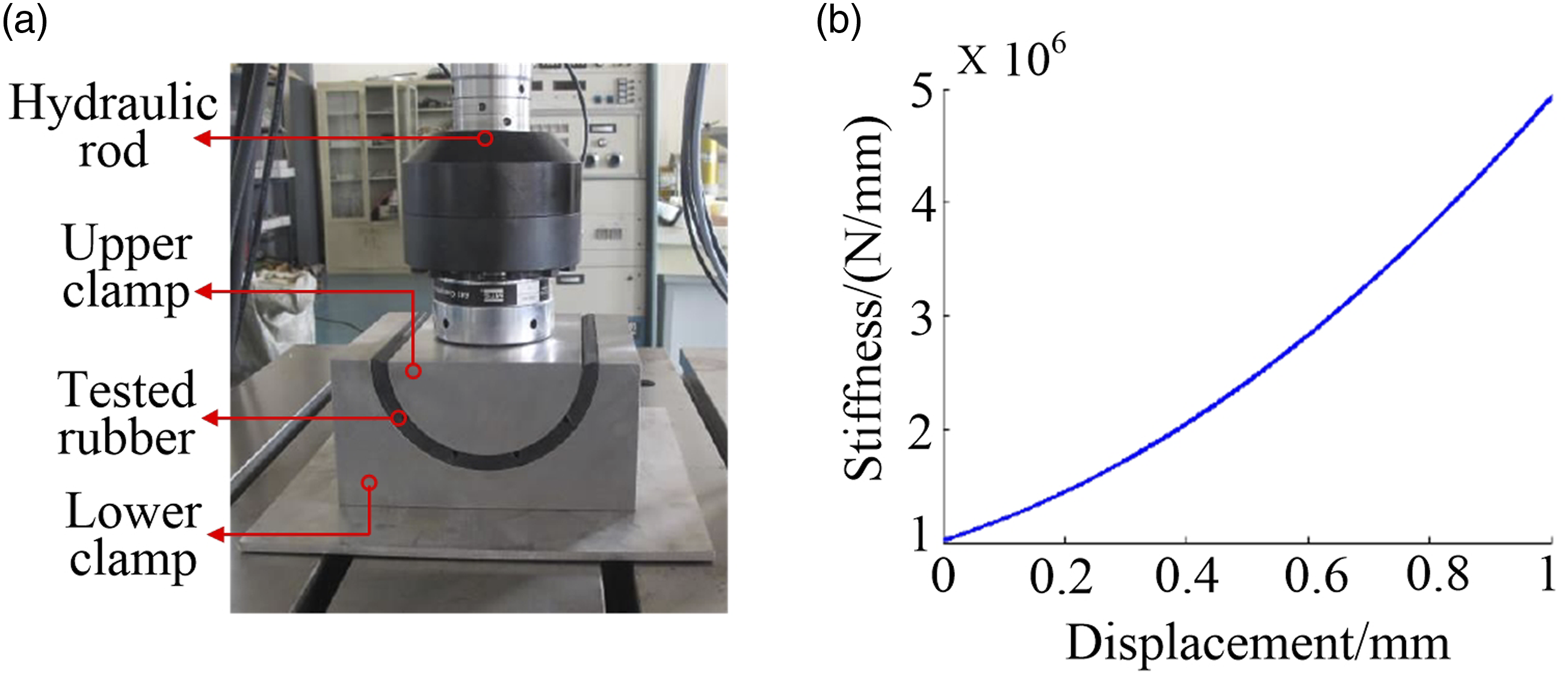
Therefore, this paper simplifies the water-lubricated rubber stern bearing-shaft system to be a 2-DOF mode-coupling simplified model considering the nonlinear stiffness of the rubber bearings, derives the analytical expressions for stick-slip vibration amplitude of the simplified model using KBM (Krylov-Bogoliubbov-Mitropolsky) method, performs the parameter discussion about the influences of friction coefficient, damping, normal force, nonlinear contact stiffness, and belt driving speed on self-excited vibration amplitudes. Different from the previously numerically investigating on the self-excited vibration of the water-lubricated rubber bearing-shaft system induced by the friction, this paper aims to provide the theoretic supports for the design and vibration controlling of the rubber stern bearing-shaft system of the marine by the analytical method.
Simplified model of the stern water-lubricated rubber bearing-shaft system
The marine stern water-lubricated rubber bearing-shaft system is seen in the Figure 2(b). When the elevations of bearings do not follow a horizontal line, it will happen that the shaft generates static deformation (as like the green line) and the pre-pressure load of the shaft becomes large. The Figure 2(a) shows enlarged section of the stern rubber bearing-shaft of the marine. The diagram of the marine stern water-lubricated rubber bearing-shaft system: (a) the enlarged section of the shaft-bearing of the ship; (b) A ship with error-elevation bearings.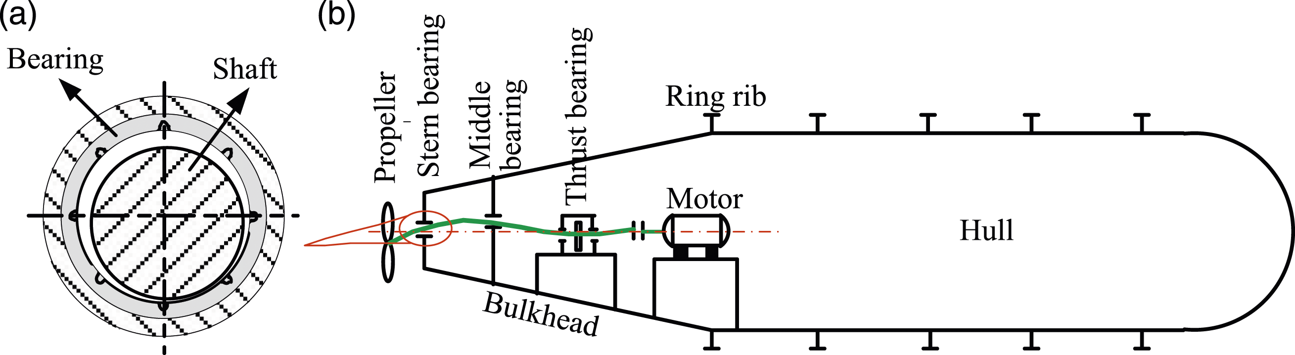
Under the condition of keeping the key dynamic characteristics similar, the stern water-lubricated rubber bearing-shaft of the marine can be described by the 2-DOF mode-coupling simplified model depicted. The simplified process is as the Figure 3. In the simplified theoretical model as the Figure 3(b), the block slider represents the shaft journal and the bearing is described by the belt and the nonlinear spring. The rotating velocity of shaft is described by the relative driving speed of the belt and regarding the speed of the slider as zero. The oblique spring represents the coupling effect between the torsional and transverse vibration of shaft. The pre-pressure load results from the error elevations of bearings; the nonlinear contact stiffness is caused by the water-lubricated rubber bearing; the horizontal and vertical oscillations, respectively, represent the torsional and transverse vibration of the shaft. The simplified process from the bearing-shaft system to 2-DOF mode-coupling simplified model: (a) simplified process; (b) 2-DOF mode-coupling simplified theoretical model.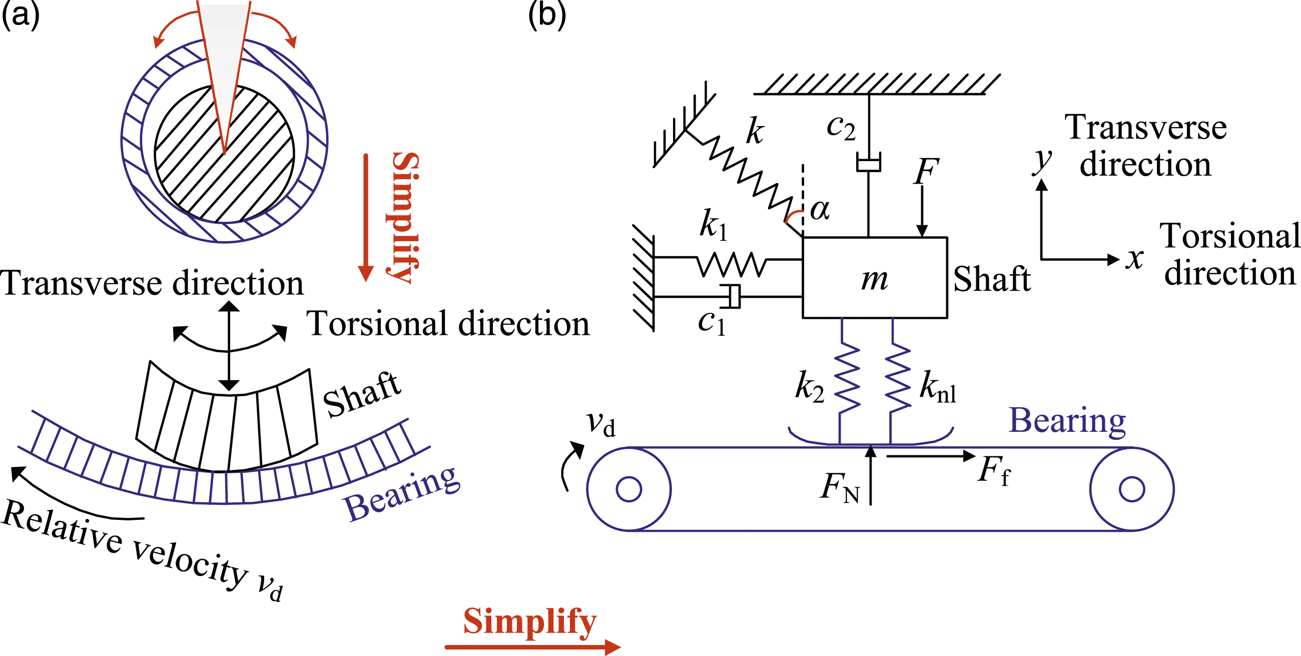
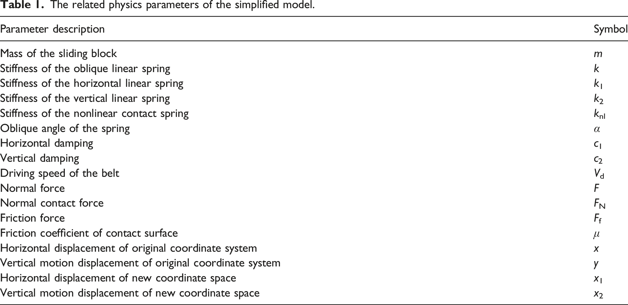
The related physics parameters of the simplified model.
The nonlinear dynamic equations of the system are as


Substitution of equations (2) and (3) into equation (1), and defining the oblique angle to be 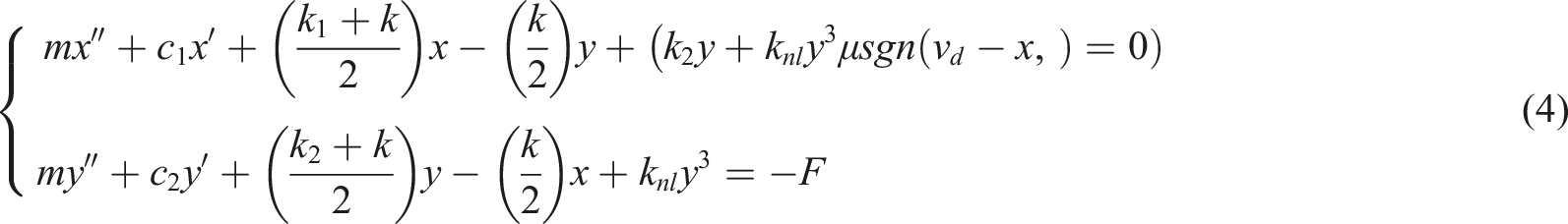
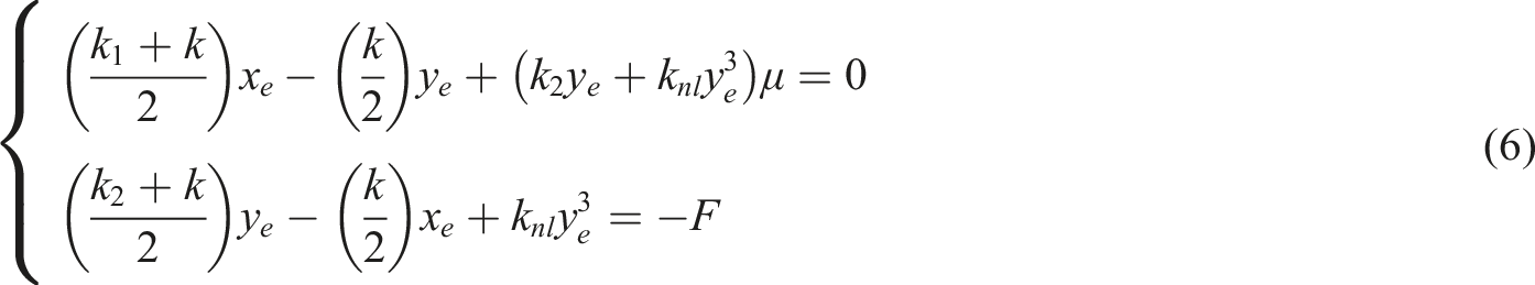
To determine the static equilibrium position, the first-order and second-order differential forms of x and y displacements are set to be zero. Substitution of equation (5) into equation (4), the nonlinear algebraic equations determining the static equilibrium position (x
e
, y
e
) are obtained, as following equation (6). Then, the static equilibrium position is capable to be obtained by solving the nonlinear algebraic equation (6) using the Newton–Raphson iterations.
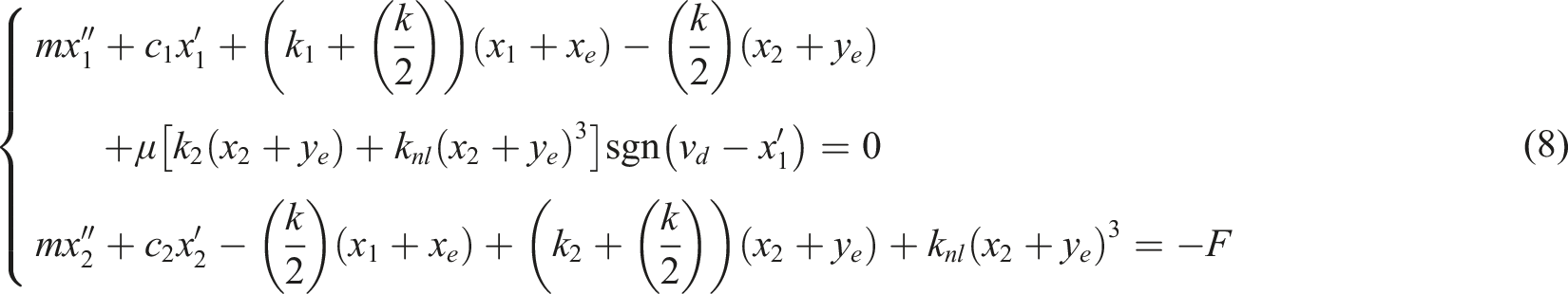
To study motions near this static equilibrium point, the new coordinate space x
1
-x
2
is set up by shift the original point as the following equation (7). In the new coordinate space, the equation (4) are rewritten as equation (8).
Substituting equation (6) into equation (8), and sorting out them, we obtain the following 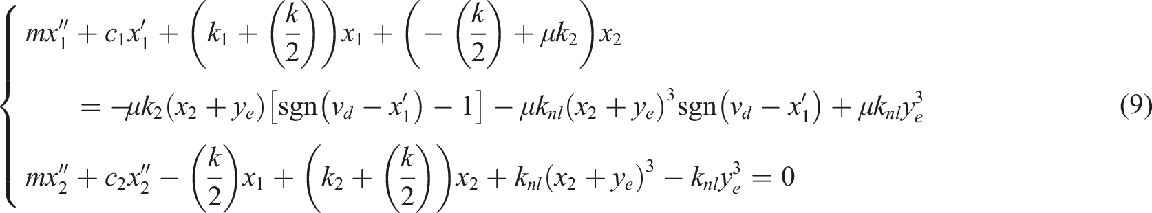
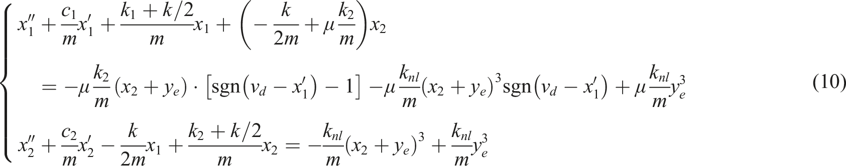

After sorting out the equation (10), the nonlinear differential governing equations of the system are as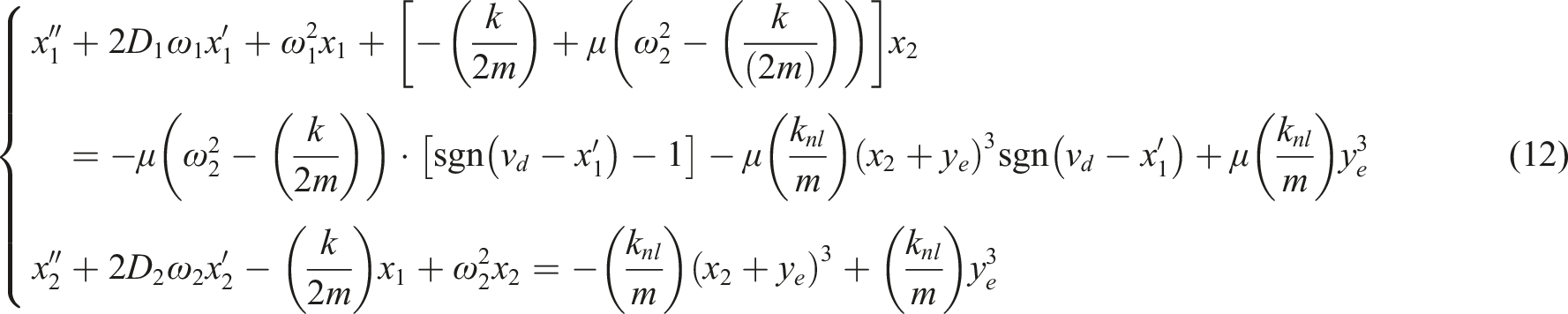
Stability study on the simplified model
It is well known that the stability behaviors of the derived system and the original nonlinear system are identical. We are therefore capable to master the stability of the original nonlinear system by investigating the stability of the derived system. The original nonlinear equation (12) of system can be linearized by the first-order Taylor series expansion around the static equilibrium position, and the linear governing equations of derived system are given as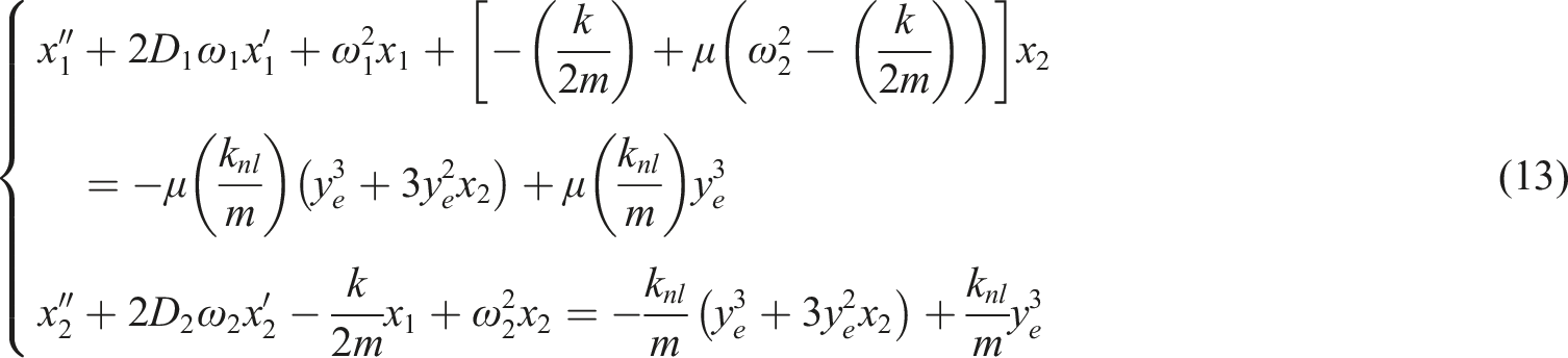
Simplifying the equation (13), they can be rewritten as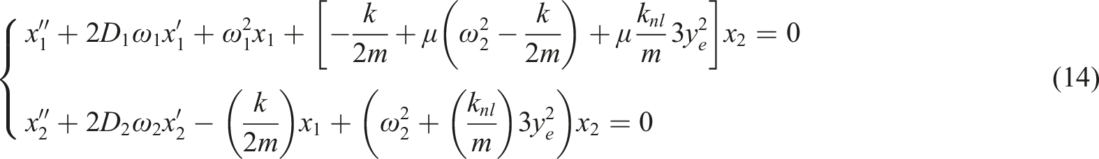
Setting four state variables as equations (15), 
The linear governing equation (14) of derived system are mapped into a state space by the equation (15). Then, the state equations of derived system are written as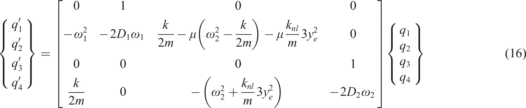
Letting function 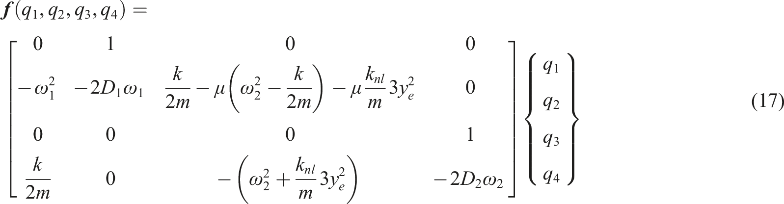
The Jacobian matrix 
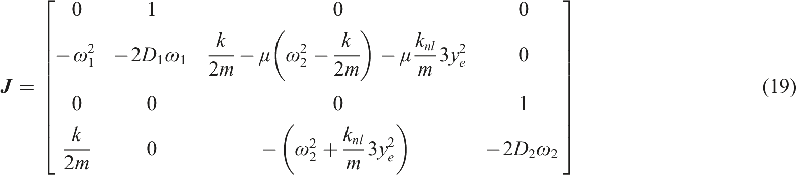
The stability of the equilibrium solution is then determined from the eigenvalue problem of the state system equation as given
The imaginary and real parts of the complex eigenvalues
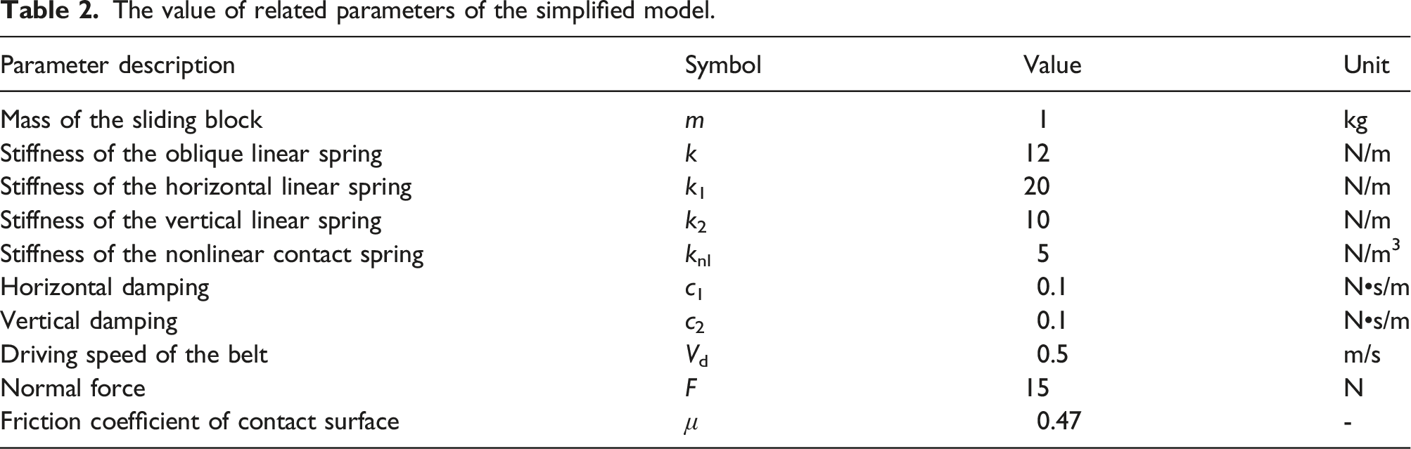
In order to investigate the instability mechanism and the influence of nonlinear stiffness, normal force and damping on the stability of the system, parameter analysis is conducted. In this section we therefore define the following fixed parameter values: the mass of the sliding block m is 1 kg; the stiffness of the oblique linear spring k, the horizontal linear spring k 1 and the vertical linear spring k 2 are, respectively, 12 N/m, 20 N/m and 10 N/m; the vertical damping c 2 is 0.1 N•s/m; the driving speed of the belt is 0.5 m/s. The parameter values of the remaining variables are flexible will be given in the corresponding cases.
Figure 4(a) and 4(b), respectively, show the 3D evolution plots of the real parts and the imaginary parts versus the μ-F parameter space with k
nl
=0 N/m3 and c
1
=0.1 N•s/m. It is obviously observed from Figure 4(b) that the system has two stable eigenmodes for friction coefficient μ<1.02, and the two eigenmodes start to merge at μ=1.02, when μ>1.02 an unstable coupling mode forms and remains. Corresponding to Figure 4(b), the real parts of complex eigenvalues in the Figure 4(a) begin to become positive from negative at the point of mode-coupling occurring, which means the instability of system takes place. This behavior is the typical mode-coupling instability, which is an important instability mechanism of friction self-excited oscillation of multi-degree-of-freedom system. Note that the points of mode-coupling occurring are actually the Hopf bifurcation points of the system. The set of the Hopf bifurcation points composites the critical curve that divides the parameter space into two subspaces, one is stable and the other is unstable. Evolution of the real parts (a) and the imaginary parts (b) versus the μ-F parameter space with k
nl
=0 N/m3 and c
1
= 0.1 N•s/m.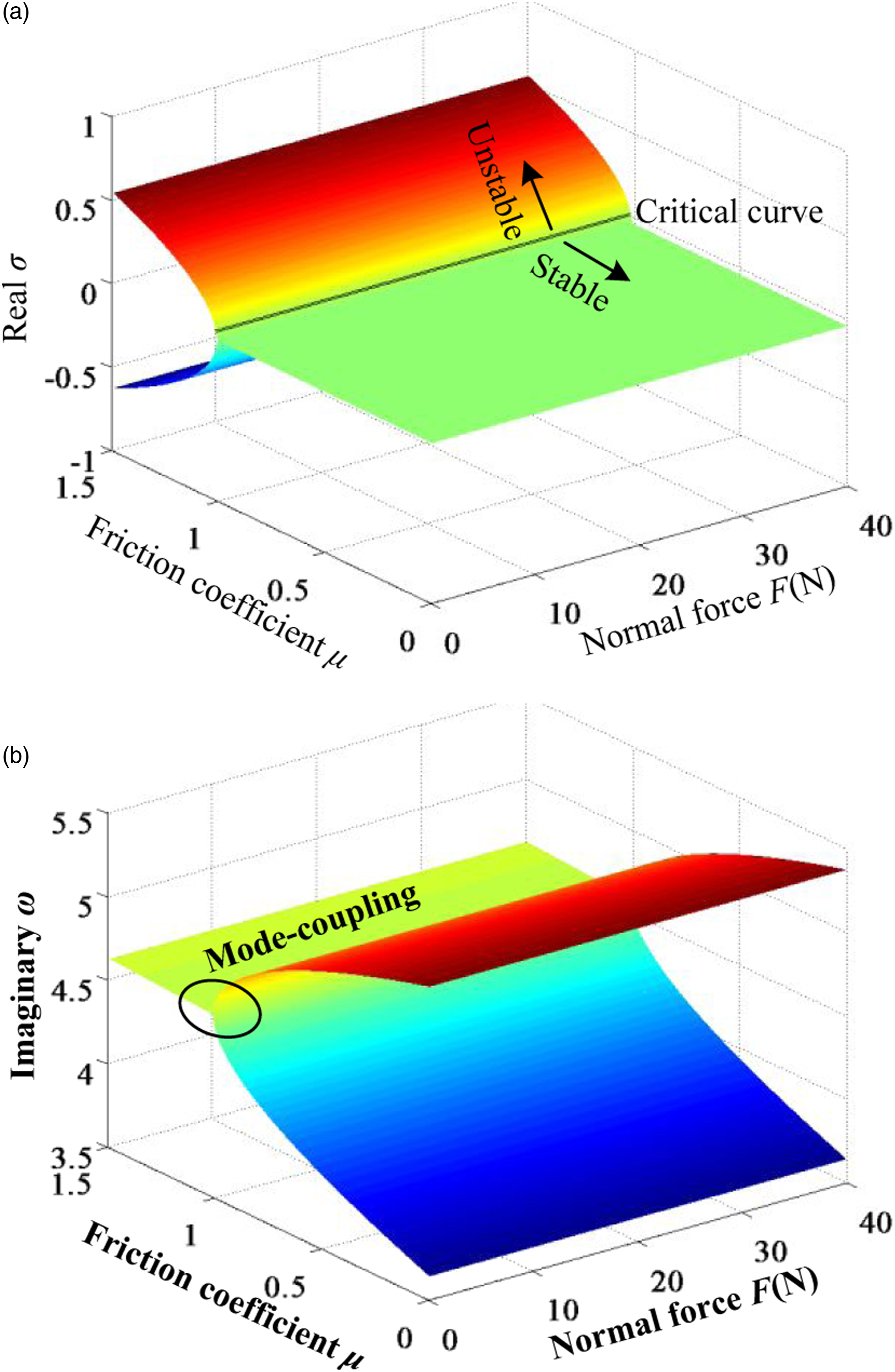
Similarly, the 3D evolution plots of the real parts and the imaginary parts versus the μ-F parameter space with k
nl
=5 N/m3 and c
1
=0.1 N•s/m are depicted in Figure 5(a) and 5(b). Different from the Figure 4, the positions of mode-coupling occurring vary with the parameter values of normal force F. Meanwhile, the critical curve is a crooked instead of a straight line, which implies the parameter values of nonlinear contact stiffness and normal force have an obvious influence on the stability of system. Evolution of the real parts (a) and the imaginary parts (b) versus the μ-F parameter space with k
nl
=5 N/m3 and c
1
= 0.1 N•s/m.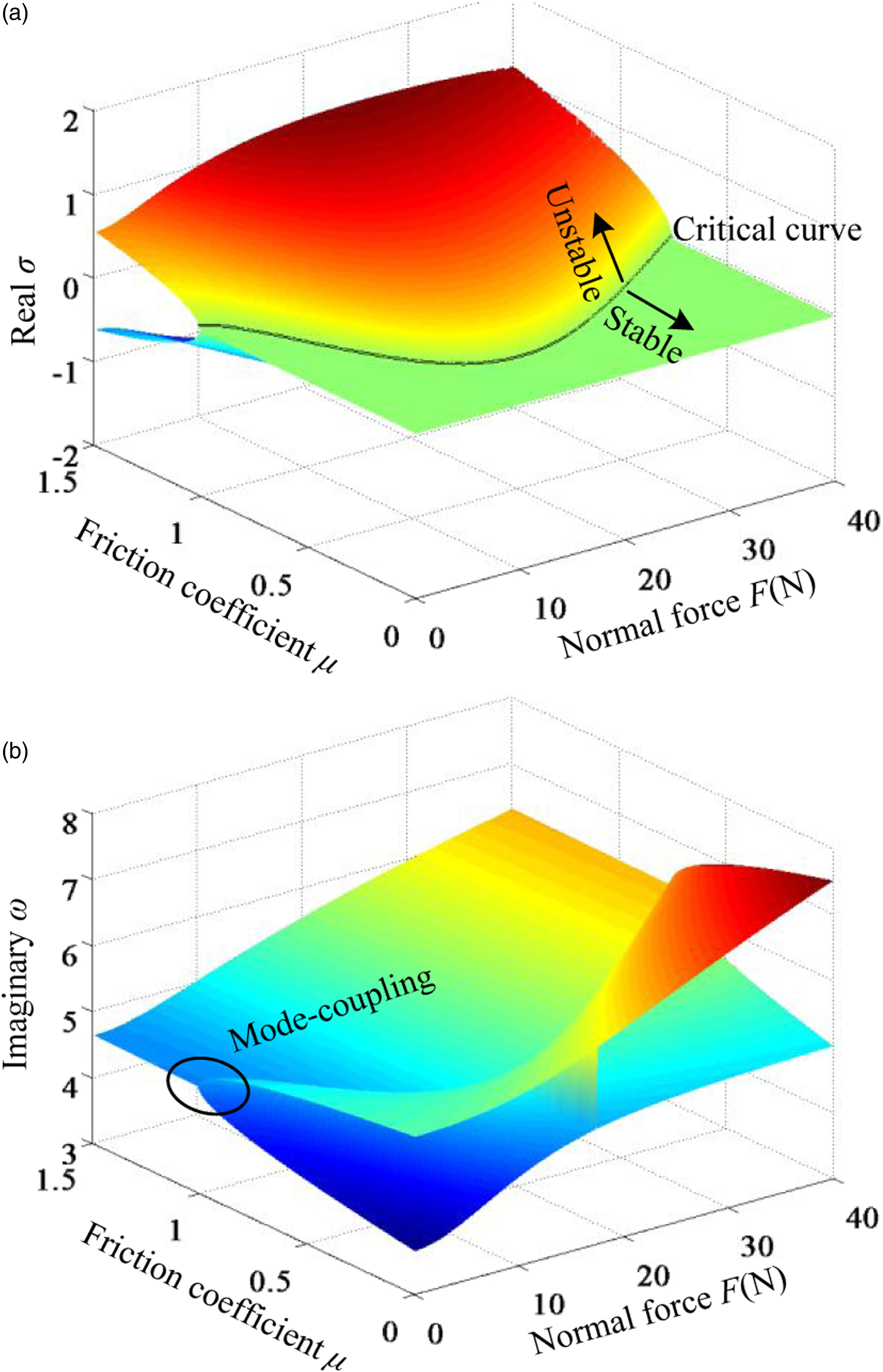
How do the system parameters influence its stability, such as nonlinear contact stiffness, normal force and horizontal damping? To answer this issue, a series of parametric studies are carried out. After the 3D evolution plots of the real parts versus the parameter space are cut by the plane of real parts σ=0, the critical curves appear, which denote the critical boundary between unstable and stable region. Mapping the critical curves into the parameter plane, the results are depicted in the Figures 6–9. The regions above each line are the unstable regions of the static equilibrium point, and the regions below each line are the stable regions. Various critical curves in the μ-F parameter plane corresponding to various nonlinear stiffness k
nl
with c
1
=0.1 N•s/m. Various critical curves in the μ-F parameter plane corresponding to various damping c
1
with k
nl
=5 N/m3. Various critical curves in the μ-c
1
parameter plane corresponding to various normal force F with k
nl
=5 N/m3. Various critical curves in the μ-c
1
parameter plane corresponding to various nonlinear stiffness k
nl
with F=5 N.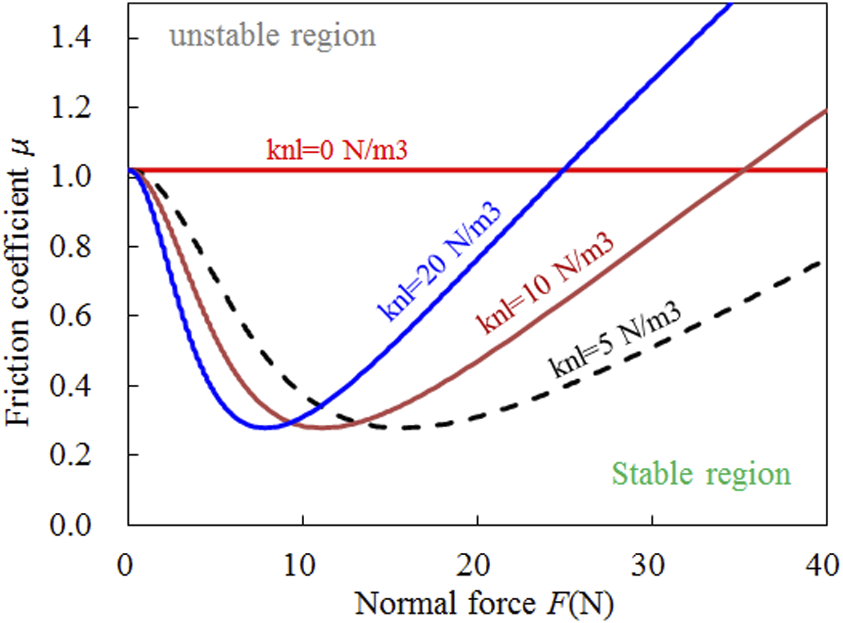
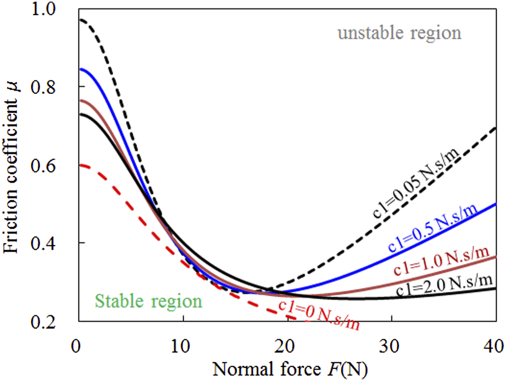
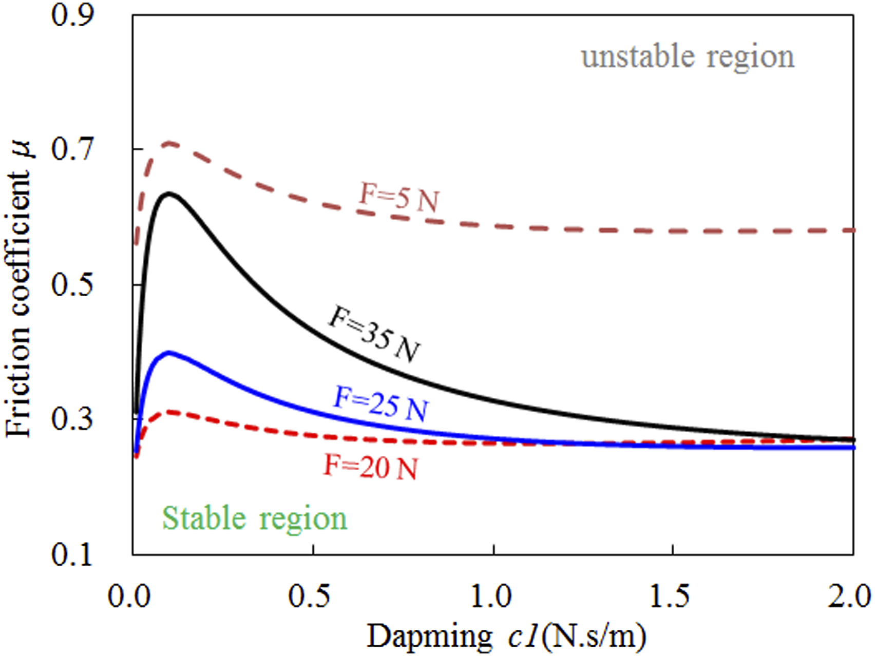
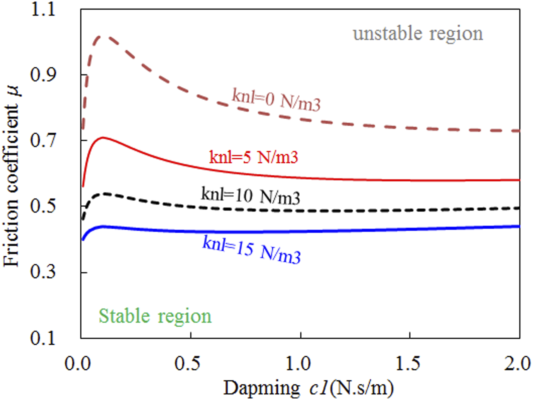
The effects of normal force and nonlinear contact stiffness on the stability are illustrated in the Figure 6. It can be seen normal force loses influence on the stability when nonlinear contact stiffness is zero, and the critical curves rapidly decrease and then increase after F=12 N when nonlinear contact stiffness is not equal to zero. Moreover, the system stability is extremely poor at F=12 N. Figure 7 shows how the normal force and horizontal damping influence system stability. With the increasing normal force, the critical curves decrease quickly and then gradually increase after F=15 N except zero horizontal damping. Especially, when horizontal damping is zero, stable region in μ-F parameter plane is the smallest, as means the system faces with the high risk of stability losing. Figure 8 presents the influences of horizontal damping and normal force on the stability. It is observed that the critical curves sharply rise and reaches a maximum value at c 1 =0.1 N•s/m, and then drop slowly with increasing horizontal damping. Furthermore, increasing normal force results in that stable region in μ-c 1 parameter plane decreases and then increases. As depicted in Figure 9, the critical curves increase drastically and then decline gradually after c 1 =0.1 N•s/m. Meanwhile, the stable region in μ-c 1 parameter plane reduces with the nonlinear contact stiffness increasing.
In conclusion, the influences of the nonlinear contact stiffness, the normal force and the horizontal damping on the system stability are extremely complex and not intuitive. Generally speaking, the stability of the system reduces sharply and then improves gradually with the normal force and the horizontal damping increasing, which implies that proper values of the nonlinear contact stiffness and the normal force can stabilize the system and some improper values may deteriorate the system stability. In addition, the effect of the horizontal damping stabilizing the system is slight once if the nonlinear contact stiffness is taken into account for the system. These characteristics of the system instability provide a significant reference for design and vibration controlling in engineering practices.
Solutions of the stick-slip vibration amplitudes of the simplified model
The KBM method is used to solve the nonlinear differential governing equations of the system in this section. After the equation (12) is sorted out, which can be rewritten as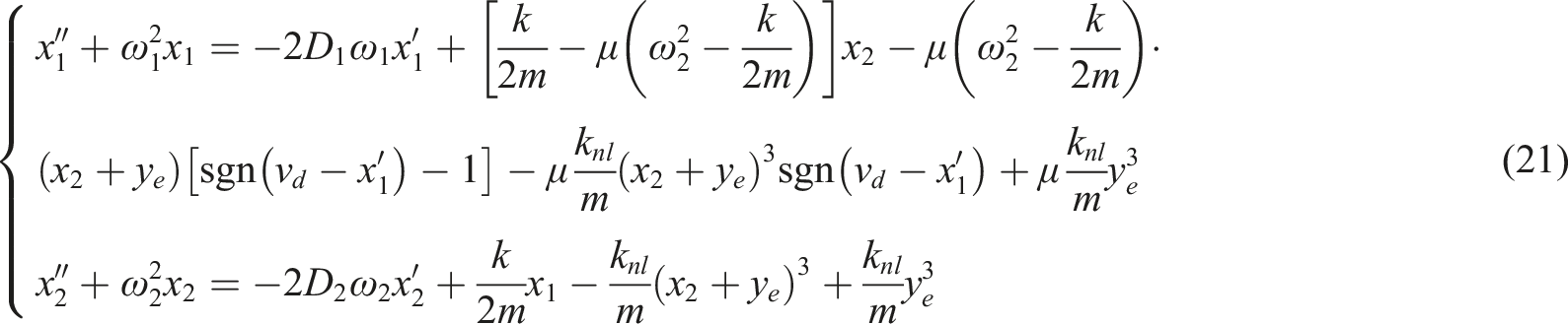
Assuming


Due to the similarity of the first and the second equation of the equation (25), the only one equation is used to derive the expressions of amplitudes and phases.
Differentiating the equation (26) with respect to time yields
Substitution of the equations (24) and (26) into the equation (27), the following equations are found.
Solving the equation (28) for 
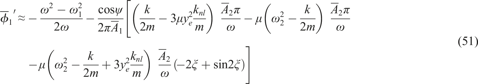
Therefore, the differentiations of amplitudes and phases with respect to time satisfy the following equations.


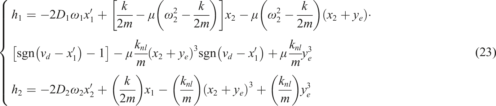
Approximations are conducted in the equation (23), after which the following equations are obtained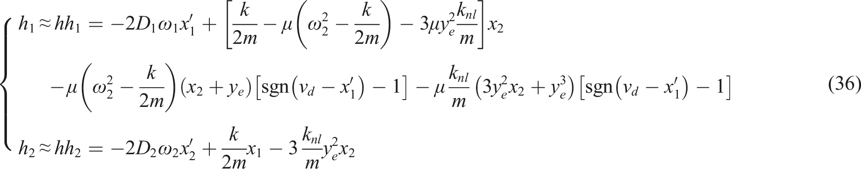
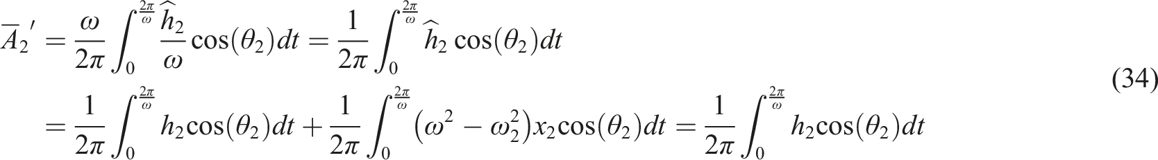
Substitution of the equation (36) into the equations (32)–(35), these equations can be rewritten as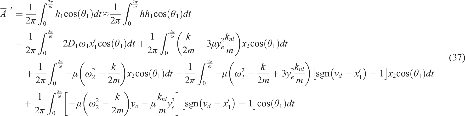
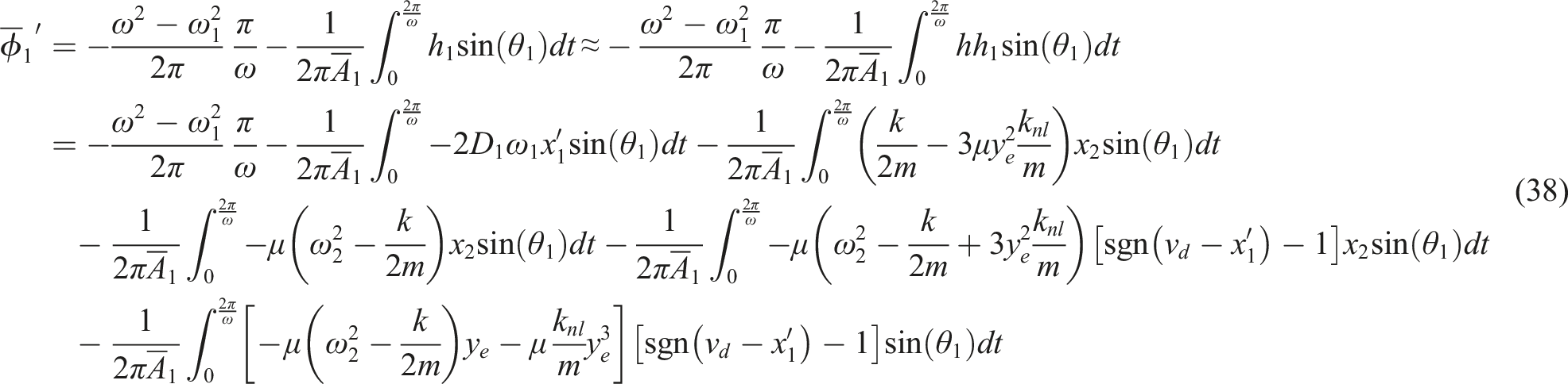
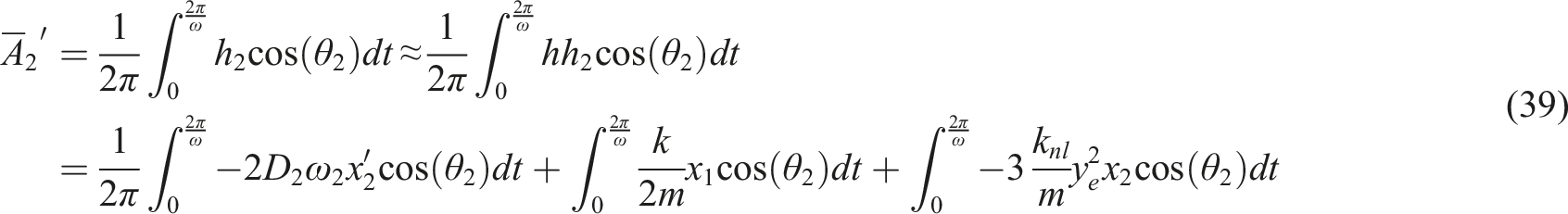
The derivative expressions of amplitudes and phases with respect to time can be obtained through performing the integrations on the equations (37)–(40). However, we have to face a problem how to perform the integrations about the sign function in these equations, which is the key point in the whole integral processes. If we only consider the pure slip vibration or ignored the stick phase of the stick-slip vibration, like the most of researchers, the vibration speed of the mass will be less than the driven speed of the belt, which means that the relative speed always is more than zero and the resulting value of the sign function will be invariant one. However, in practical engineering, the stick-slip phenomenon exists indeed and cannot be ignored. It means the vibration speed of the mass will be less or more than the driven speed of the belt, which leads to that the value of the sign function will be variant. Therefore, this paper separately considers the pure slip and the stick-slip vibration, and provides the analytical expressions for pure slip and stick-slip vibration amplitude in the following subsections.
The analytical expressions corresponding to the pure slip vibration amplitudes
When we only consider the pure slip vibration or ignored the stick phase of the stick-slip vibration, the sign function keeps invariable one. The integration about the sign function therefore satisfies the following equations.
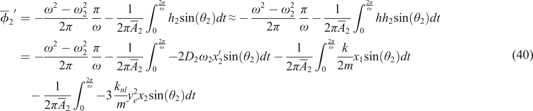
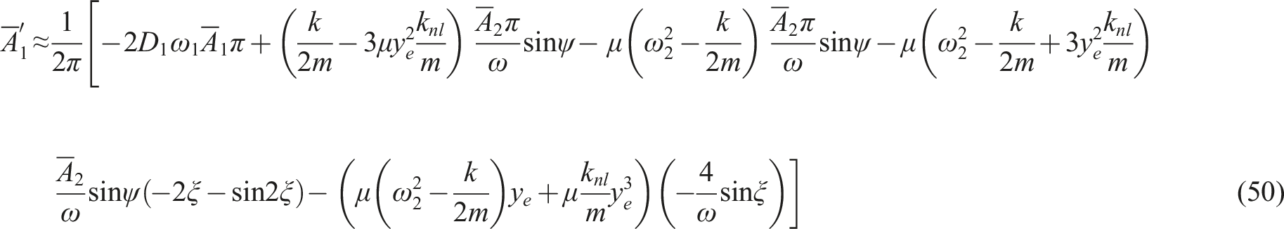
Substitution of the equation (41) into the equations (37)–(40), and performing the complex mathematical operations, the resulting equations are given as


The analytical expressions corresponding to the stick-slip vibration amplitudes
Actually, the stick-slip phenomenon exists indeed and cannot be ignored, which leads to the value of the sign function variant. Hence, the integration about the sign function is broken into three parts. That is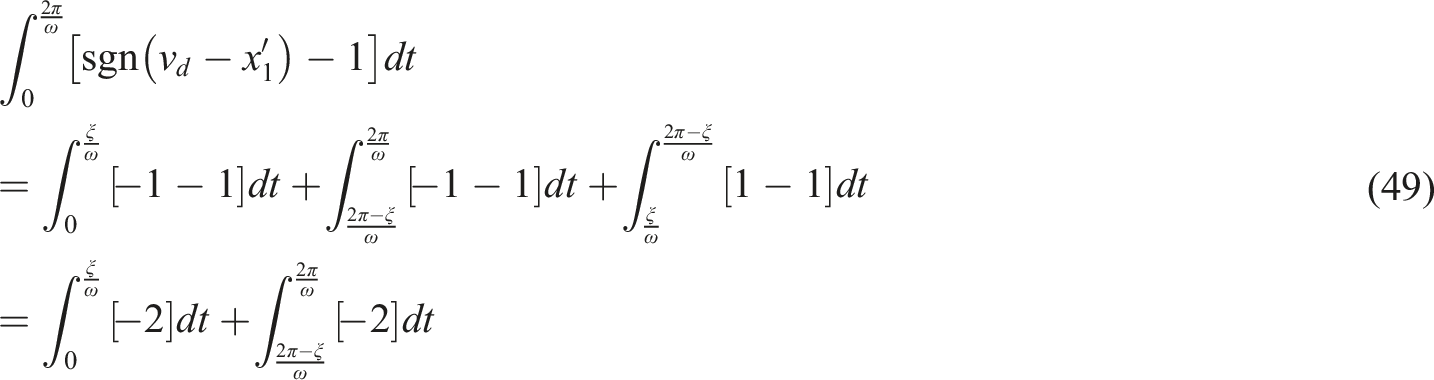


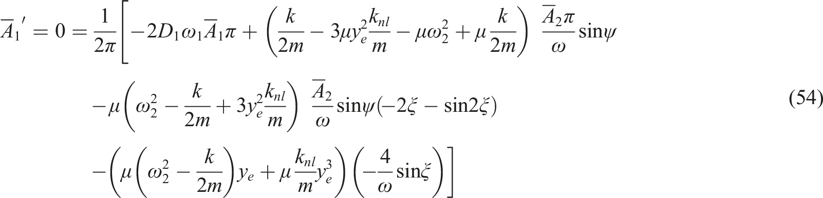

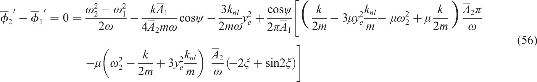
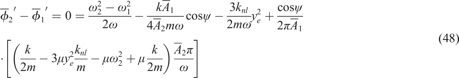
The solutions of the analytical expressions
Respectively, there are the three unknown variables
Numerical validation and parameter discussion
The value of related parameters of the simplified model.
Numerical validation
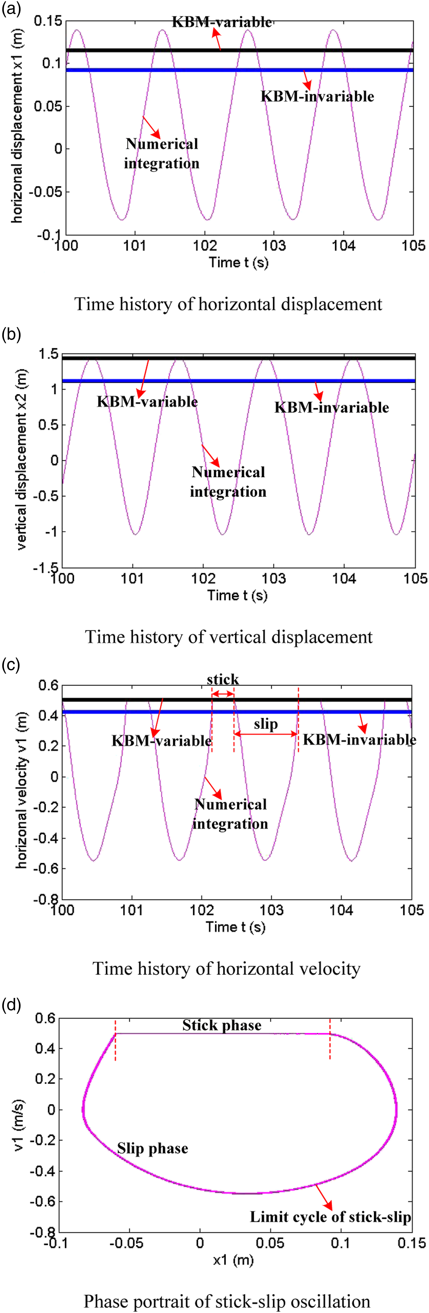
The Figures 10–11 depict the comparisons of the horizontal and vertical oscillation amplitudes of displacement and velocity between analytical prediction and numerical integration with friction coefficient μ=0.31 and μ=0.43. The blue thick line represents the analytical predictions considering the invariable sign function; the black thick line represents the analytical predictions considering the variable sign function, and the red thin line represents numerical integration. Comparisons of the horizontal and vertical oscillation amplitudes of displacement and velocity between analytical prediction and numerical integration with μ=0.31. (a) Time history of horizontal displacement; (b) Time history of vertical displacement; (c) Time history of horizontal velocity; (d) Phase portrait of pure slip oscillation. Comparisons of the horizontal and vertical oscillation amplitudes between analytical prediction and numerical integration with μ=0.43. (a) Time history of horizontal displacement; (b) Time history of vertical displacement; (c) Time history of horizontal velocity; (d) Phase portrait of stick-slip oscillation.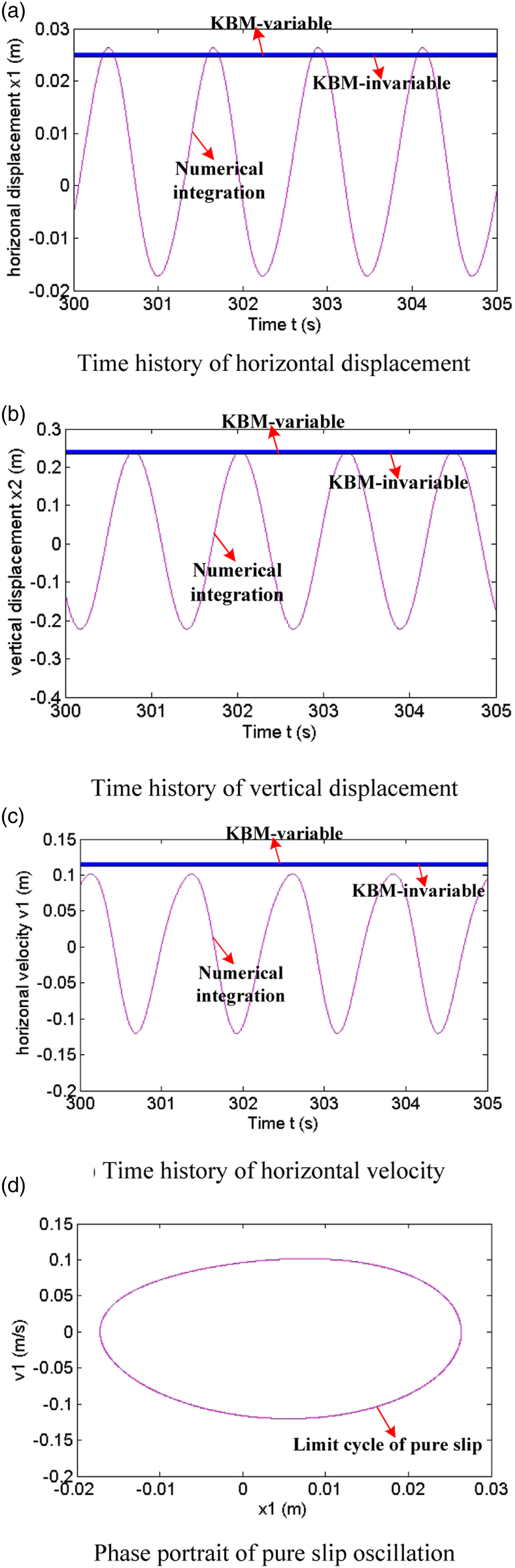
The self-excited pure slip oscillation is depicted in Figure 10. When the self-excited oscillation reaches the steady state, the displacement and velocity responds in the time interval from 300 s to 305 s are chosen to be shown in Figure 10. It is obvious that the agreement of the analytical predictions (blue thick line and black thick line) with numerical integration (red thin line) is perfectly good. Furthermore, the analytical predictions considering the invariable sign function (blue thick line) and the invariable sign function (black thick line) coincides, which exposes they are identical when the type of the self-excited oscillation is pure slip. As shown in the Figure 10(d), the limit-cycle behavior of pure slip oscillation appears which is induced by the friction force of the system.
The self-excited stick-slip oscillation is shown in Figure 11. Similarly, when the self-excited oscillation reaches the steady state, the displacement and velocity responds in the time interval from 100 s to 105 s are chosen to be depicted in Figure 11. The analytical predictions considering the variable sign function well matches with numerical integration, and the distinction between the analytical predictions considering the invariable sign function is not small. It is revealed that the supposition of the invariable sign function may be untenable, when the type of the self-excited oscillation is stick-slip.
Thus, no matter the type of the self-excited oscillation is pure slip or stick-slip, the analytical predictions considering the variable sign function has a good accuracy, although its calculation is complex. To the contrary, the analytical predictions considering the invariable sign function can maintain its precision only in the condition of self-excited pure slip oscillation, because it neglects the contribution of the stick effect to the displacement and velocity responds. Additionally, the error of analytical predictions also comes from the harmonic assumption of KBM. However, the horizontal and vertical oscillations are not actually strict harmonic behavior, which can be seen in the Figure 10(d) and 11(d).
We have analyzed the stability property of the two-degree-of-freedom model with nonlinear stiffness and normal force via linear stability analysis which is used by most of researchers, in section “Stability study on the simplified model”. Generally, the theory of linear stability analysis is true. However, to the stability analysis of the friction-induced self-excited vibration model described in this paper, it is not exactly accurate, which has been raised in the form of open questions by Kruse.
23
In order to expose the questions, this paper therefore reanalyzes the stability property of the model in the situation of k
nl
=10 N/m3 as is one of the critical curves shown in the Figure 6, through the numerical stability analysis. Observed from the Figure 12(a), it is obvious that the trend of the two critical curves is same, but they are not absolutely identical to each other. There is a conflicting region between the two critical curves in which the stability property obtained from linear and numerical stability analysis is opposite. Which result about the stability property of the model is right in the end? Maybe, the responds of the red dot (corresponding to the parameters F=35 N and μ=0.87) located in the conflicting region in the Figure 12(a) can tell us answer. The Figure 12(b) depicts the transient-state responds of the vertical displacement at the red dot with a slightly initial condition. We can see from the Figure 12(b) and 12(d) that the stick-slip self-excited vibration occurs and it reaches its steady state after 200 s, instead the response converges into the static equilibrium point. In addition, the Figure 12(c) shows the comparison of the steady-state horizontal velocity, respectively, obtained from the KBM and numerical integration, which imply that KBM also has a good precision in this situation. Now, we can answer the above question. To the stability analysis of the friction-induced self-excited vibration model, numerical stability analysis is absolutely right. But it will take numerous computational efforts. The linear stability analysis only can make the qualitative analysis, by which the exactly quantitative bounds of the stability region cannot be obtained. The stability analysis in the conflicting region between the two critical curves. (a) The comparison of critical curves obtained from linear and numerical stability analysis in the μ-F parameter plane with k
nl
=10 N/m3, (b) Transient-state time history of vertical displacement at the red dot of the left figure, (c) Steady-state time history of horizontal velocity, (d) Phase portrait of stick-slip oscillation.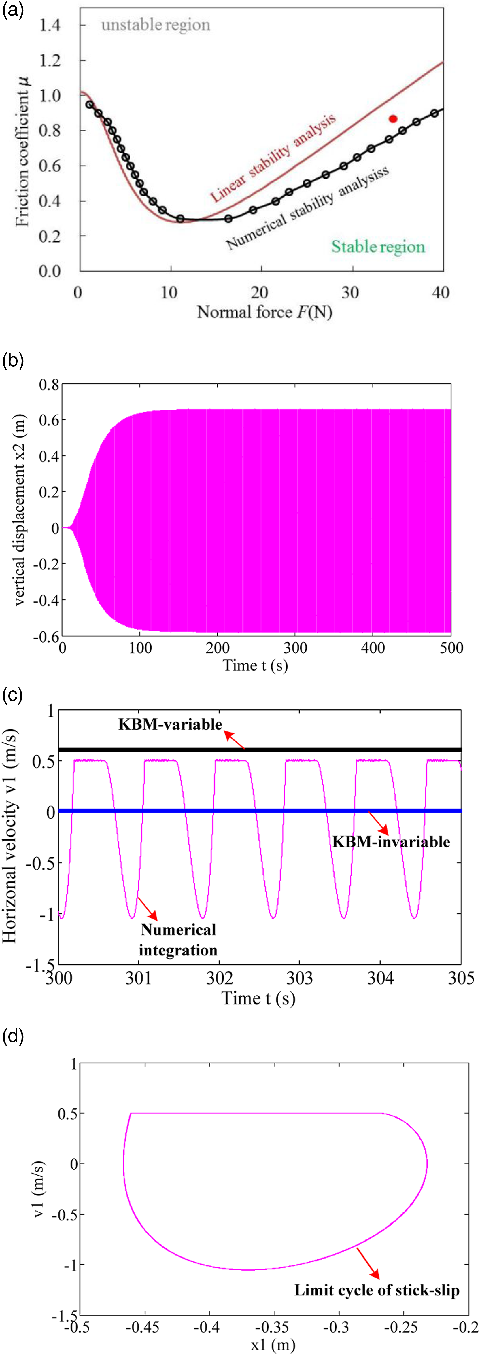
Parameter discussion
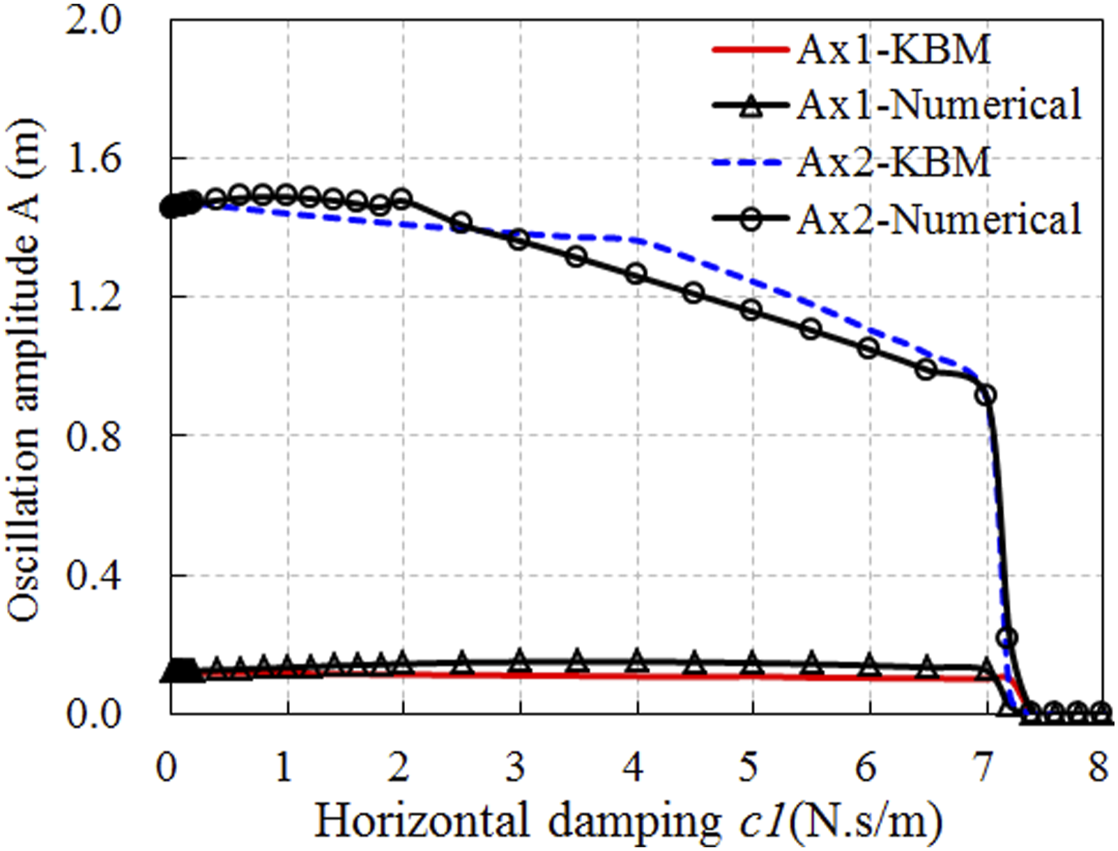
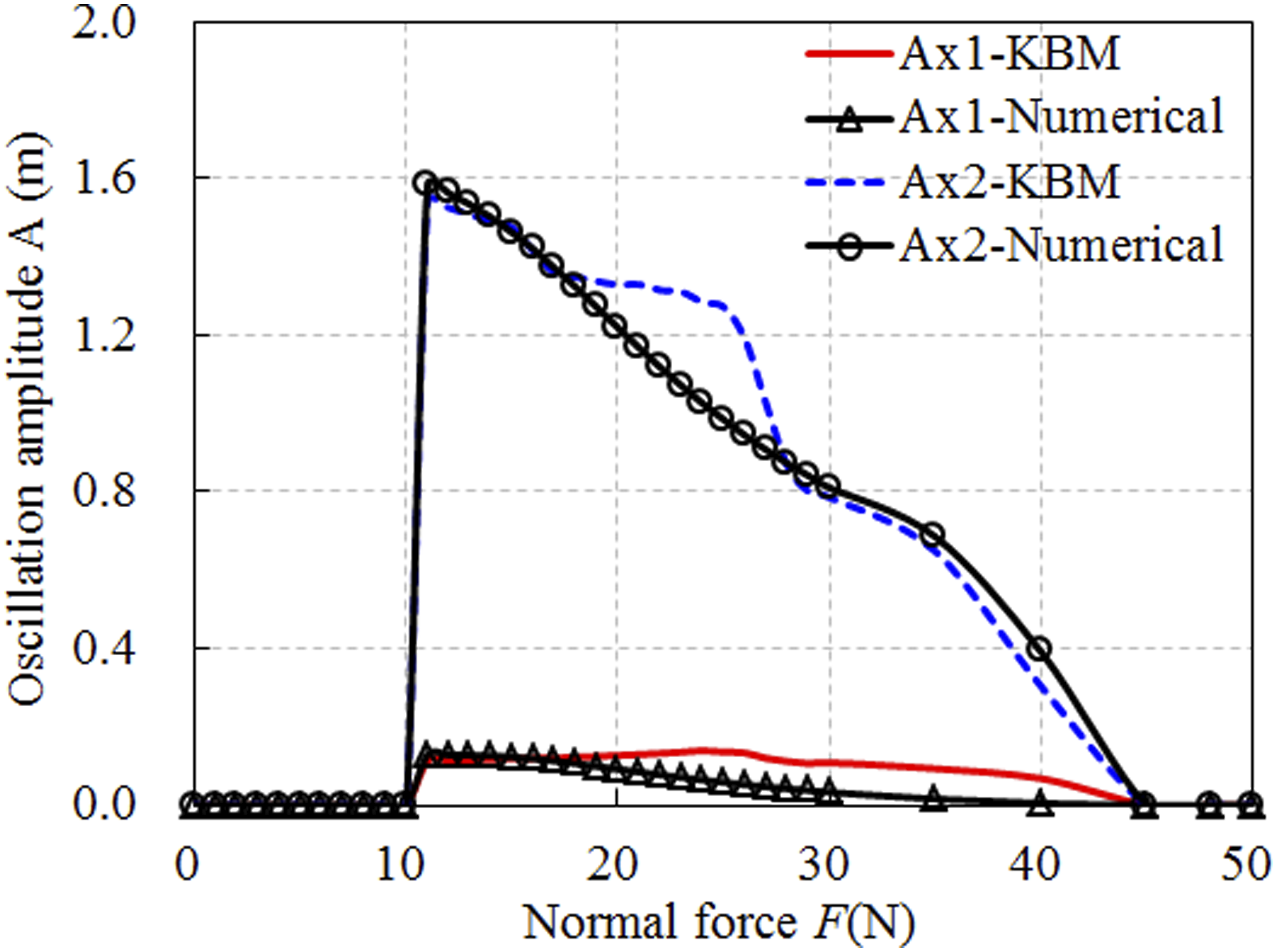
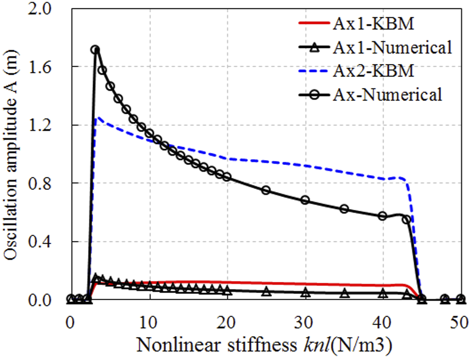
The effects of a series of system parameters on the horizontal and vertical oscillation amplitudes are illustrated in the Figures 13–16. It is seen from the Figures 13–14 Horizontal and vertical oscillation amplitudes for various friction coefficient μ. Horizontal and vertical oscillation amplitudes for various horizontal damping c1. Horizontal and vertical oscillation amplitudes for various normal force F. Horizontal and vertical oscillation amplitudes for various normal stiffness knl.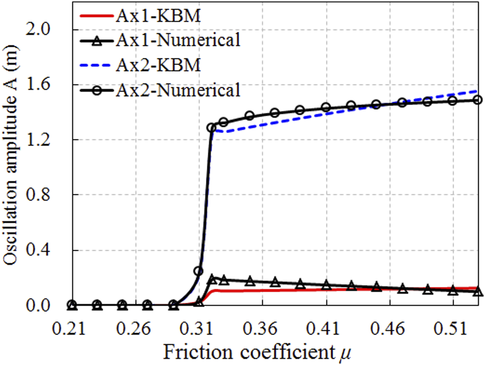
Conclusions
The originality of the present work, in this paper, is that two types of analytical expressions for stick-slip vibration amplitudes in the friction-induced self-excited model with nonlinear contact stiffness are derived by using KBM method. Moreover, the friction-induced instability behaviors of the model are exposed.
The influences of the nonlinear contact stiffness, the normal force and the horizontal damping on the system stability are extremely complex and not intuitive. The appropriate values of the nonlinear contact stiffness and the normal force can stabilize the system. Furthermore, the effect of the horizontal damping stabilizing the system is slight once if the nonlinear contact stiffness is taken into account for the system.
When the self-excited oscillation reaches the steady state, it is obvious that the agreement of the analytical predictions considering the variable sign function is generally good and the analytical predictions considering the invariable sign function has a weak precision. The error mainly comes from the harmonic assumption of KBM. However, the horizontal and vertical oscillations are not actually strict harmonic behavior. According to the influences of the system parameters on self-excited vibration amplitudes, the system can keep the steady state of static equilibrium or the oscillations with small amplitude if some appropriate parameter values of the variables are chosen, which is helpful to control the friction-induced vibration of the water-lubricated rubber bearing-shaft system.
Especially note that the present method for predicting the stick-slip vibration amplitude in mode-coupling friction self-excited model with nonlinear contact stiffness must satisfy the limited condition: the stick-slip oscillation has the approximate or absolute harmonic behavior.
Footnotes
Declaration of conflicting interests
The authors declared no potential conflicts of interest with respect to the research, authorship, and publication of this article.
Funding
The author(s) disclosed receipt of the following financial support for the research, authorship, and/or publication of this article: research is supported by Fundamental Research Funds for the Central Universities (3072023CFJ0501).