Sage Journals: Discover world-class research

Abstract

The effectiveness of an active noise barrier is heavily dependent on the positioning of secondary sources and error sensors. Typically, these components are located at the edge of the barrier; however, research suggests that alternative distributions may improve the performance of the active barrier. This paper utilizes a genetic optimizer to determine optimal transducer locations based on specific criteria. Two approaches are employed: the Two-step approach which, first identifies optimal control source positions and then seeks the best error microphone locations, and the Multi-parameter approach, which optimizes all active noise control parameters simultaneously. The acoustic fields of primary and secondary sources are analyzed for various numbers of control sources progressively increasing from 2 to 10 units. Results indicate that the Multi-parameter approach achieves higher outcomes and requires less computational effort. This approach is more desirable than the Two-step approach. The best configuration for the active noise barrier is determined to be control sources and error microphones placed at a height below the barrier’s edge and are distributed with an interval between a half and a full wavelength. The number of error sensors should be close to the number of secondary sources and both transducers should be placed at the farthest distance from the barrier surface, but oppositely. Furthermore, the study shows that when the primary noise source is close to the barrier adjacent transducers should not be spaced uniformly.

Keywords

Active noise barrier genetic algorithms transducers’ location optimization extra insertion loss noise cancellation noise attenuation

Introduction

Research has shown that active noise control significantly enhances the performance of acoustic barriers at low-frequency noise bands.^1–4 Despite the existence of various parameters that affect the efficiency of active noise barriers, few studies have optimized them.^5–7 Some of these parameters include the number, location, and distance between adjacent control sources and error microphones. Previous investigations have typically examined the impact of these parameters separately. For instance, Omoto et al.⁸ studied the effect of the space between error microphones when located on the barrier’s edge. They showed the active control system performs more efficiently when the distance between the error microphones is less than the noise half wavelength. Similarly, Shao et al.⁹ demonstrated that more attenuation can be achieved by increasing the number of error microphones compared to control sources when using the same setup as Ref. 8. Niu et al.¹⁰ studied the effect of distance between control sources and error microphones on the performance of an active noise barrier with a rectangular profile.¹⁰ They suggested an optimal value for this distance when the transducers were placed next to the top edge of the barrier.

Previous studies have focused on improving the performance of active noise barriers by examining only a few configurations or variables. Sohrabi et al.^11,12 addressed this issue by systematically calculating the insertion loss for numerous candidate positions of control sources and error microphones in an infinite active noise barrier. They found that the active noise control system is more efficient when control sources are placed at the incident side and below the top edge of the barrier, and error microphones are located in barrier’s the shadow zone. However, this method is time-consuming and several variables were not optimized.

To address these limitations, an optimization method can be employed to determine the best configuration for transducers. Various optimization methods such as Bracketing, Local descent, First-order, Annealing algorithms, and Genetic algorithms can be used to optimize different parameters of an objective function. While some methods utilize the derivative of the objective functions to determine optimal parameter values, these methods are not effective for non-differential objective functions or those functions that derivatives can only be computed for a single or specific domain.¹³ On the other hand, differential-free optimization algorithms such as Direct, Evolutionary, and Stochastic algorithms operate directly on the objective functions. Genetic algorithms (GAs) which are global optimization methods fall into this category.^14–16

Although previous studies have optimized passive barriers using genetic algorithms,^17–21 no studies have reported using these optimization algorithms for active noise barriers. This study aims to optimize different parameters of an active noise barrier using genetic algorithms. The objective is to determine the optimal positions for transducers of an active noise barrier to achieve maximum attenuation at a target area in the shadow zone. This study optimizes parameters such as the positions, intervals, and number of control sources and error microphones.

The primary objective of this article is to improve the performance of active noise sound barriers. The study employs a diffraction model to simulate the propagation of sound waves around the barrier and proposes two optimization approaches to determine the optimal location of transducers of the active noise barrier. In the following section the theory utilized for the diffraction model is explained in detail. The optimization methodologies employed in this study are defined in Methodology. Subsequently, the results obtained through these methodologies are presented and analyzed. Finally, in the Conclusions section, the main findings of this study are summarized, highlighting the significance of the optimization approaches proposed in methodologies.

Theory

Diffraction model

The sound field at an arbitrary receiver point around a barrier depends on the relative positions of the noise source and the receiver, but generally, it can be decomposed into diffracted, reflected, and direct fields.^11,22

In the present study, the diffracted field of an infinite barrier is calculated by Macdonald’s model (equation (1))

P_{D} = {\frac{k^{2} ρ c}{4 π} q}_{0} [s i g n (ζ_{1}) \int_{| ζ_{1} |}^{\infty} \frac{H_{1}^{(1)} (k R_{1} + s^{2})}{\sqrt{s^{2} + 2 k R_{1}}} d s + s i g n (ζ_{2}) \int_{| ζ_{2} |}^{\infty} \frac{H_{1}^{(1)} (k R_{2} + s^{2})}{\sqrt{s^{2} + 2 k R_{2}}} d s]

(1)

where

k

(m⁻¹) is the wavenumber,

q_{0}

(m³.s⁻¹) is the complex strength of the source,

ρ

(kg.m^{− 3}) and c (m.s⁻¹) are the air density and speed of sound in air, respectively.

H_{1}^{(1)} ()

is the Hankel function of the first kind,

R_{1}

and

R_{2}

are the distances (in meters) from the source and its barrier image to the receiver, respectively.

s

is the variable of the contour integral and the limits of the two contour integrals in equation (1) are determined according to

ζ_{1} = s i g n (| θ_{s} - θ_{r} | - π) \sqrt{k (R^{'} - R_{1})}

(2)

ζ_{2} = s i g n (θ_{s} + θ_{r} - π) \sqrt{k (R^{'} - R_{2})}

(3)

where

s i g n ()

is the sign function, and

θ_{s}

and

θ_{r}

are the source and receiver angles with the top edge of the barrier, respectively, and

R^{'}

is the shortest path from the source to the receiver through the edge.

In regard to the direct and the reflected pressures, they are computed by the following expression

P_{d} = (\frac{- i k ρ c}{4 π} q_{0}) \frac{e^{i k R_{1}}}{R_{1}}

(4)

P_{r} = (\frac{- i k ρ c}{4 π} q_{0}) \frac{e^{i k R_{2}}}{R_{2}}

(5)

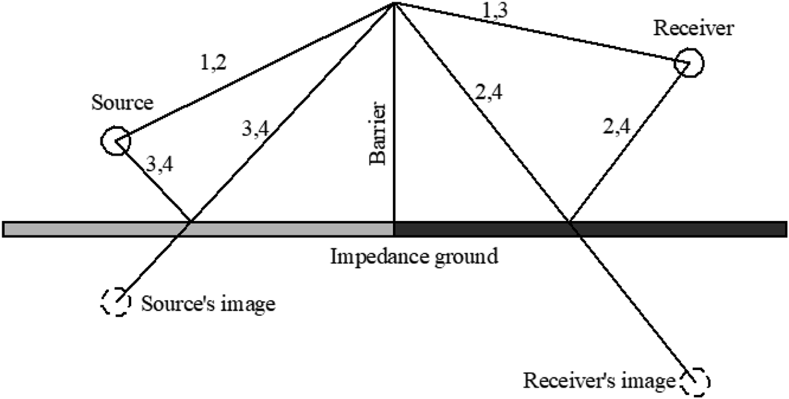
The effect of the soil’s reflection can be considered based on the image method.²³ Figure 1 shows all possible paths from a source to a receiver in the shadow zone. The total pressure ( $P_{T}$ ) at the receiver is the summation of the pressures of all these wavefronts and describe as $P_{T} = P_{1} + {Q_{r} P}_{2} + Q_{s} P_{3} + Q_{r} Q_{s} P_{4}$ , where $Q_{s}$ and $Q_{r}$ are the spherical wave reflections at the source and receiver sides, respectively, and depend on the acoustical characteristic of the ground and the source/receiver geometry.^24,25

Figure 1.

Diffracted wave paths from a source to a receiver point in the shadow zone of a barrier.²²

Minimization of square pressure at error microphones

In an active noise control system, the sound pressure at a given point is the superposition of the primary fields and the secondary fields, which are the contributions of secondary sources. Equation (6) denotes the total sound pressure at a point

P_{t o t} = Z_{P} q_{P} + Z_{s} q_{s}

(6)

where

Z_{P}

is the vector of complex acoustic transfer impedances of the primary source with a strength of

q_{P}

, and

Z_{s}

is an

M \times N

matrix, corresponds to the transfer impedance matrix of

N

control sources at the positions of

M

points. In equation (6),

q_{s}

denotes the vector of the complex strength of the control source,²⁶ and is determined by minimizing the total squared pressure at the error microphones. The total squared acoustic pressure is expressed in equation (7)

J_{p} = P^{H} P = {{| q_{p} |}^{2} Z}_{P}^{H} Z_{P} + q_{p}^{*} Z_{P}^{H} Z_{s} q_{s} + q_{s}^{H} Z_{s}^{H} Z_{p} q_{P} + q_{s}^{H} Z_{s}^{H} Z_{s} q_{s}

(7)

The unique value for the strengths of control source that minimizes equation (7) is given by²⁶

q_{s} = - {(Z_{s}^{H} Z_{s})}^{- 1} (Z_{s}^{H} Z_{p} q_{P})

(8)

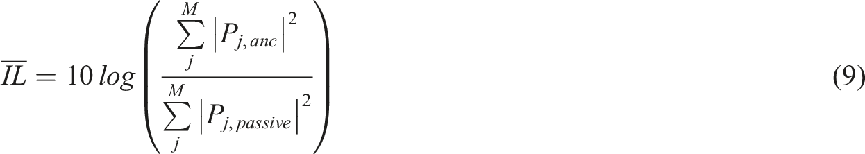
Average insertion loss in an area

In this work, the performance of the active noise barrier is evaluated by determining the average extra attenuation achieved in the target zone through active means. This value is computed as the difference between the average squared pressure level at the target zone after and before the application of active noise control, as expressed in equation (9)

\bar{I L} = 10 \log (\frac{\sum_{j}^{M} {| P_{j, a n c} |}^{2}}{\sum_{j}^{M} {| P_{j, p a s s i v e} |}^{2}})

(9)

where

P_{j, a n c} = Z_{\Pr} q_{P} + Z_{s r} q_{s}

represents the sound pressure at M observation points in the target zone after active noise control is activated, which is calculated as the sum of

Z_{\Pr} q_{P}

and

Z_{s r} q_{s}

. Here,

Z_{\Pr}

and

Z_{s r}

denote the impedance matrices of primary and secondary sources, respectively.

P_{j, p a s s i v e}

refers to the total sound pressure at the same observation points prior to the implementation of active noise control. Therefore, throughout this study,

\bar{I L}

refers to the extra noise reduction contributed by the active noise control system.

Methodology

There are various methods to solve differential equations. The variational iteration algorithm^27–30 is a numerical method that involves the construction of an iterative series solution that converges to the exact solution of the differential equation. The algorithm first represents the differential equation’s unknown solution with a trial function before using the variational principle to generate a series of correction functional equations. With each iteration, the approximation of the solution to these correction equations is improved.

The Riccati transformation method is another mathematical method for resolving linear second-order differential equations.³¹ In this approach, a change in variables, more specifically a Riccati transformation, is used to convert a second-order differential equation into a first-order differential equation. Following transformation, the equation can be solved using methods that are common for first-order differential equations. The Riccati transformation method is especially beneficial for resolving linear differential equations with variable coefficients or nonhomogeneous terms.

However, when the search space is large or the equation is complex it may be more advantageous to use alternative optimization techniques such as Genetic Algorithms (GAs). These algorithms are able to explore a large number of potential solutions in a relatively efficient manner. The objective of this study is to optimize variables of the equation (9) simultaneously, in a way to have the highest noise reduction by the active cancellation for the barriers. In this regard, genetic algorithms have been used to find the optimal values for each parameter. These algorithms enable to optimize multiple parameters at the same time.

Model description

The present study employs a genetic optimizer implemented in the MATLAB Global Optimization Toolbox³² to perform optimizations. The objective function during the optimization procedure is the averaged extra insertion loss achieved by the active noise control system at a designated target area (equation (9)). The target area has dimensions of 10 $\times$ 8 m² and a height of 1.65 m, located behind a $2.5$ m tall, thin, rigid infinite barrier. The effectiveness of the active noise barrier is evaluated by calculating the average noise reduction at 15 discrete observation points distributed evenly at the target zone. A primary monopole noise source with a tonal noise of 200 Hz is situated at a fixed point 7 m away from the barrier. The primary source has a complex strength of $q_{p}$ = 0.0674 (m³.s⁻¹), equivalent to a power output of 1 W.

Figure 2 schematically illustrates the target zone, barrier, and primary noise source. The “Error microphone zone” and “Control source zone” in the figure delineate the permissible areas for placing the candidate positions of error microphones and control sources, respectively.

Figure 2.

A schematic model of the target zone and observation points located behind the barrier.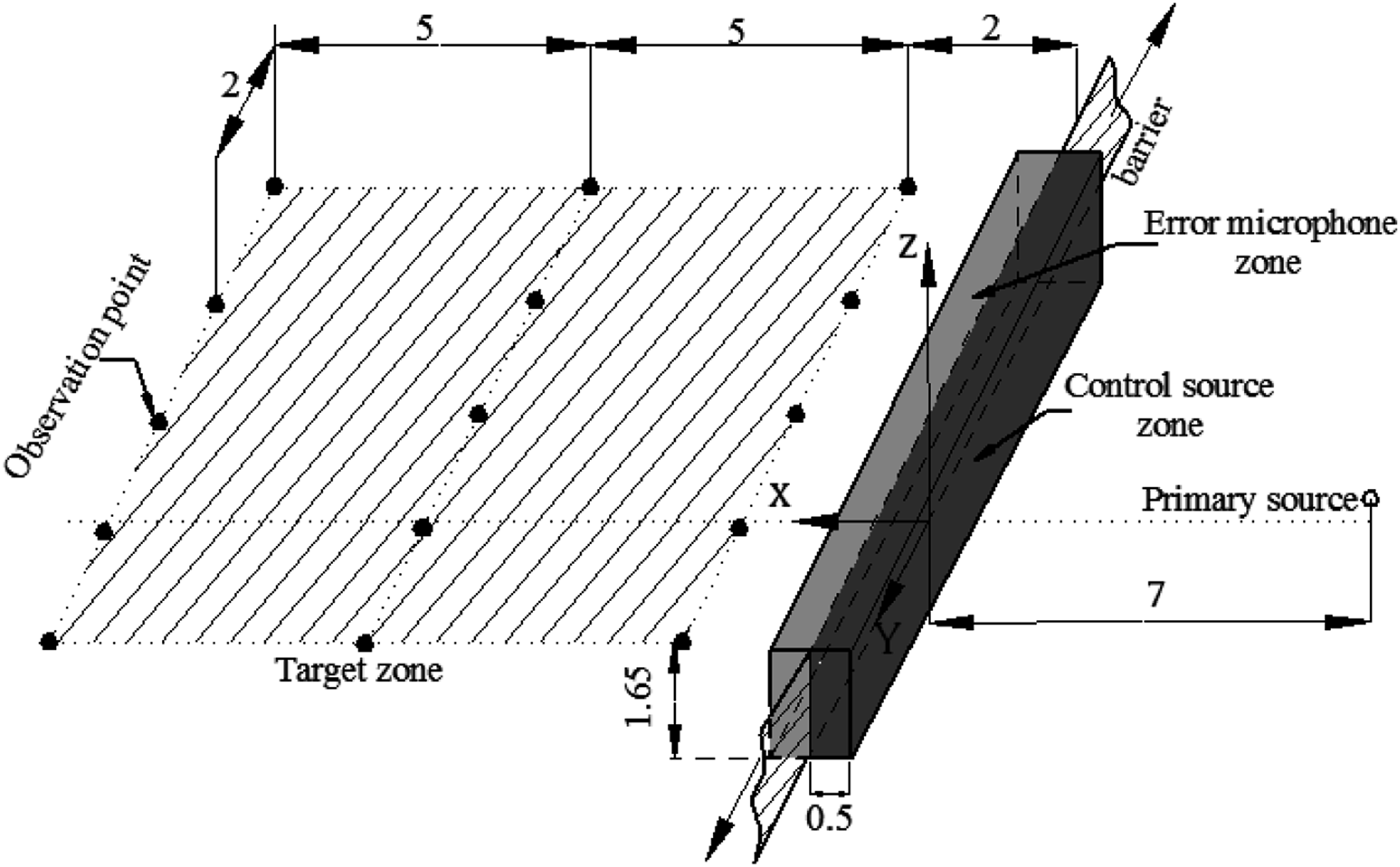

As demonstrated in a previous study¹¹ the performance of an active noise barrier can be improved by positioning the control sources on the incident side and below the barrier’s edge while ensuring that all observation points in the target zone are outside the direct field of the control sources. Error microphones, on the other hand, should be situated below the height of the barrier on the shadow side.

Based on the conclusions of Ref. 11 in this study the candidate positions are defined by a grid with 0.1 m spacing in the “Error microphone” and “Control source” zones. These candidate positions were selected deliberately close to the surface of the barrier to facilitate the real-world application of active noise barriers and to minimize the disruption to surrounding activities.

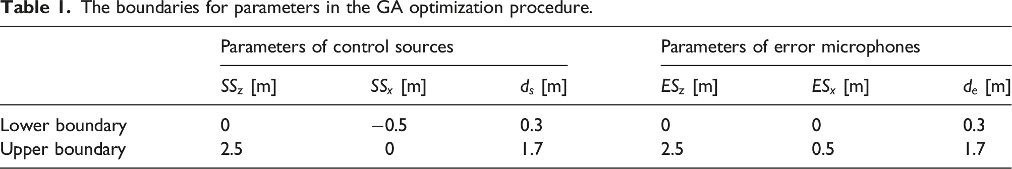
The optimization parameters considered in this study include the X- and Z- coordinates of the secondary sources’ location ( ${S S}_{x}$ and ${S S}_{z}$ ), the X- and Z- coordinates of the error sensors’ placement ( ${E S}_{x}$ and ${E S}_{z}$ ), and the distances between adjacent control sources ( $d_{s}$ ) and error microphones ( $d_{e}$ ). Figure 3 shows the optimization parameters schematically.

Figure 3.

Geometric parameters of an active noise barrier.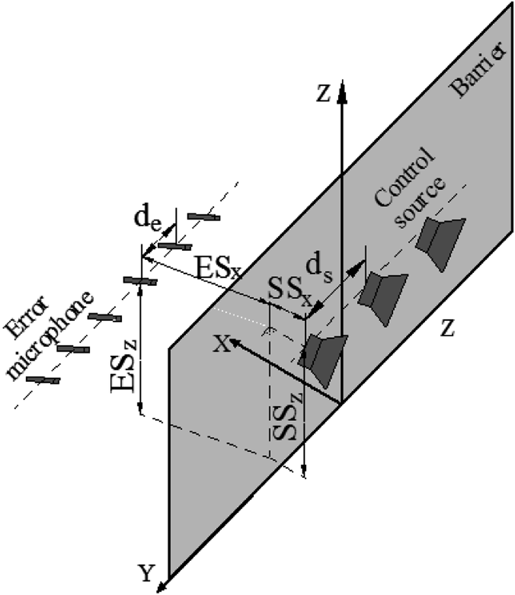

The optimization procedure sets the upper boundaries of

d_{s}

and

d_{e}

to be smaller than the wavelength,³³ while the lower boundary is set at 0.3 m, taking into account the practical size of low-frequency loudspeakers. Table 1 provides an overview of the parameters, as well as their corresponding lower and upper boundaries for use in the optimization process.

Table 1.

The boundaries for parameters in the GA optimization procedure.

	Parameters of control sources			Parameters of error microphones
	${S S}_{z}$ [m]	${S S}_{x}$ [m]	$d_{s}$ [m]	${E S}_{z}$ [m]	${E S}_{x}$ [m]	$d_{e}$ [m]
Lower boundary	0	−0.5	0.3	0	0	0.3
Upper boundary	2.5	0	1.7	2.5	0.5	1.7

Optimization approaches

The present study employs two approaches to determine the optimal values of the control parameters using the genetic algorithm GA, namely the “Two-step” and “Multi-parameters” approaches. The optimization procedure is terminated when either the maximum generation of 100 or a convergence tolerance of 10⁻⁶ is reached. All optimization procedures are carried out using a high-performance cluster with a 2 GHz Intel® Xeon® Gold 6138 CPU (counting 40 cores), however, the calculations are performed with 10 cores.

Two-step approach

The “Two-step” approach used in this study^11,33–35 involves optimizing the parameters through two separate steps using genetic algorithms. In the first step, the parameters associated with control sources ( ${S S}_{x}$ , ${S S}_{z}$ , and $d_{s}$ ) are optimized to minimize the squared pressures at observation points in the target zone, by calculating the complex strengths of secondary sources using equation (8). This step determines the optimal placement for the control sources, ensuring the maximum achievable noise level reduction in the target zone.¹ In the second step, the parameters for the error microphones ( ${E S}_{x}$ , ${E S}_{z}$ , and $d_{e}$ ) are optimized with the control sources positioned at the locations found in the previous step. The total squared pressure is minimized at the error microphone positions located in the Error microphone zone shown in Figure 2. The optimal values for the error microphone parameters are those that result in the highest average insertion loss at observation points in the target zone. The objective function for the GA optimizer during both steps is the average insertion loss at the observation points in the target zone (equation (9)).

Multi-parameter approach

In the “Multi-parameter” approach, all parameters listed in Table 1 are considered as design variables and the GA optimizes them simultaneously in a single step. The objective function for this approach is the average insertion loss achieved in the target zone, which is the same as in the “Two-step” approach.

Results and discussions

The implementation of the GA is first validated by comparing its outputs with the results obtained from the model presented in Ref. 11. Once the validation is confirmed, the two optimization approaches are applied to different numbers of control sources. Finally, the results of both approaches are compared and discussed.

Model validation

To validate the correctness of the optimization procedure, the outputs of the genetic algorithm are compared with the results presented in Ref. 11, which used 10 control sources and 41 error microphones arranged linearly in a zone close to the barrier. The optimization with GA is performed by the Two-step approach with the same conditions presented in Ref. 11 for the street area as the target zone.

The optimizations were repeated for various distances between the noise source and the barrier (

d_{pr}

), and the results are summarized in Table 2.

Table 2.

Validation of genetic algorithms with Ref. 11.

	Results of GA			Results of Ref. 11
$d_{pr}$ [m]	( ${S S}_{x}$ , ${S S}_{z}$ ) [m]	( ${E S}_{x}$ , ${E S}_{z}$ ) [m]	IL [dB]	( ${S S}_{x}$ , ${S S}_{z}$ ) [m]	( ${E S}_{x}$ , ${E S}_{z}$ ) [m]	IL [dB]
1	(−0.5, 0)	(0.5,2.4)	16.4	(−0.5, 0)	(0.5,2.4)	16.4
2.5	(−0.5,1.8)	(0.5,1.1)	11.9	(−0.5,1.8)	(0.5,1.1)	11.9
4	(−0.5, 1.8)	(0.5,0.9)	10.9	(−0.5, 1.8)	(0.5,0.9)	10.9
5.5	(−0.5, 1.8)	(0.4,0.4)	9.9	(−0.5, 1.8)	(0.4,0.4)	9.9
7	(−0.5, 1.8)	(0.4,0.2)	9.3	(−0.5, 1.8)	(0.4,0.2)	9.3

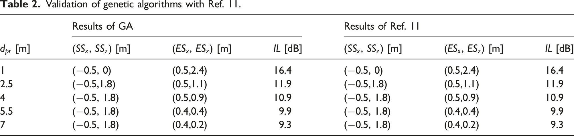
According to Table 2, under identical conditions, the positions of transducers found by the GA optimizer align with those found by the repetitive method outlined in Ref. 11 The calculations utilized a constant spacing of 0.2 m between adjacent transducers ( $d_{s} = d_{e} = 0.2$ m). Nevertheless, for further optimization, these parameters are regarded as variables.

Optimization with the two-step approach

Step 1: Square pressure minimization at the observation points

The study at hand does not treat the number of control sources as a variable because it is widely recognized that a higher number of control sources leads to greater reductions in the target zone.^36,37 Nonetheless, beyond a certain threshold, an increase in secondary sources has only a marginal effect on the rise of attenuation.²⁷ In light of this, to investigate the impact of the number of control sources on their optimal locations and the effectiveness of the active noise barrier, optimizations are conducted with increasing numbers of control sources, N_s, progressively increasing from 2 to 10 units.

Table 3 displays the optimized values for parameters associated with control sources (

{S S}_{z}

{S S}_{x}

, and

d_{s}

), along with the average insertion loss at the target zone and the calculation time. These values are obtained via the GA after the initial stage of the Two-step approach.

Table 3.

Optimized control source at 200 Hz obtained via the two-step approach.

$N_{s}$	2	3	4	5	6	7	8	9	10
${S S}_{z}$ [m]	0.5	0	2.5	0.4	0.4	0.9	1.7	2.5	2.5
${S S}_{x}$ [m]	−0.5	−0.5	−0.5	−0.5	−0.5	−0.5	−0.5	−0.5	−0.5
$d_{s}$ [m]	1.5	1.0	1.3	0.5	0.5	0.5	0.5	0.5	0.6
${I L}_{S t e p 1}$ [dB]	3.1	4.3	8.4	12.4	12.1	17.3	18.6	21.1	20.9
Time_Step1 [h]	0.8	1.0	2.2	3.4	4.1	5.2	7.3	8.6	9.6

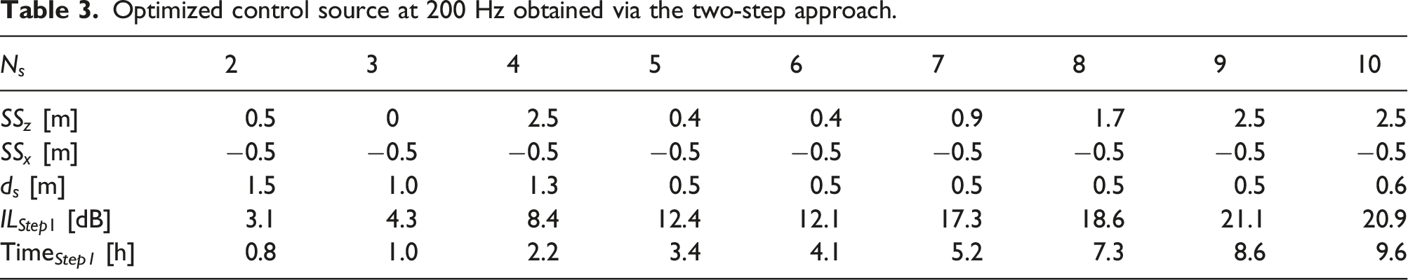
In general, higher insertion losses are observed as the number of control sources increases, as has been reported in prior research.^36,37 However, the results presented in Table 3 suggest that this general trend may not hold if the locations of control sources during the optimization process are restricted to specific numbers of candidate positions or regions. For instance, the optimizations at $N_{s} = 6$ , and $N_{s} = 10$ in Table 3 yield lower insertion losses than $N_{s} = 5$ , and $N_{s} = 9$ , respectively. In order to ensure that the genetic algorithms have obtained global optimal solutions, the optimization calculations were repeated multiple times for cases with a small number of variables. The results of these repetitions remained consistent or exhibited minor variations.

Additionally, Table 3 demonstrates that there is no consistent trend for the Z- coordinate of the secondary sources across different numbers of control sources. However, the optimal positions for SSx typically are farthest from the barrier and closer to the noise source.

Previous empirical research^8,38 found that when the distance between control sources is less than half a wavelength, better results are achieved. However, Elliot et al.³⁹ recently demonstrated that this distance should be less than a complete wavelength. In this study, the optimal spacing between control sources is mostly slightly less than half a wavelength ( $\frac{λ}{2} = 0.86$ m), which aligns with previous findings. However, when only a few control sources are included in the active control system, the GA outputs indicate that this spacing can be expanded beyond half a wavelength for better results, but they are always less than a wavelength.³⁹

Figure 4, depicts the distributions of insertion loss achieved at different heights of the shadow zone with 10 control sources placed at the positions presented in Table 3. In this figure, the rectangle dash represents the projection of the target zone on each plane. As shown, for planes above the target zone (heights greater than Z = 1.65 m), the cancellation is concentrated in the target zone. However, below the height of the target zone, the noise is attenuated in regions further from the center of the target zone.

Figure 4.

(Color online) IL [dB] distribution at various heights in the barrier’s shadow zone, with 10 control sources at the position presented in Table 3. Heights include (I): 2.5 m, (II): 2.0 m, (III): 1.5 m, (IV): 1.0 m, (V): 0.5 m, (VI): ground level. Rectangular dash indicates the projection of the target area on each plane. (Print in color).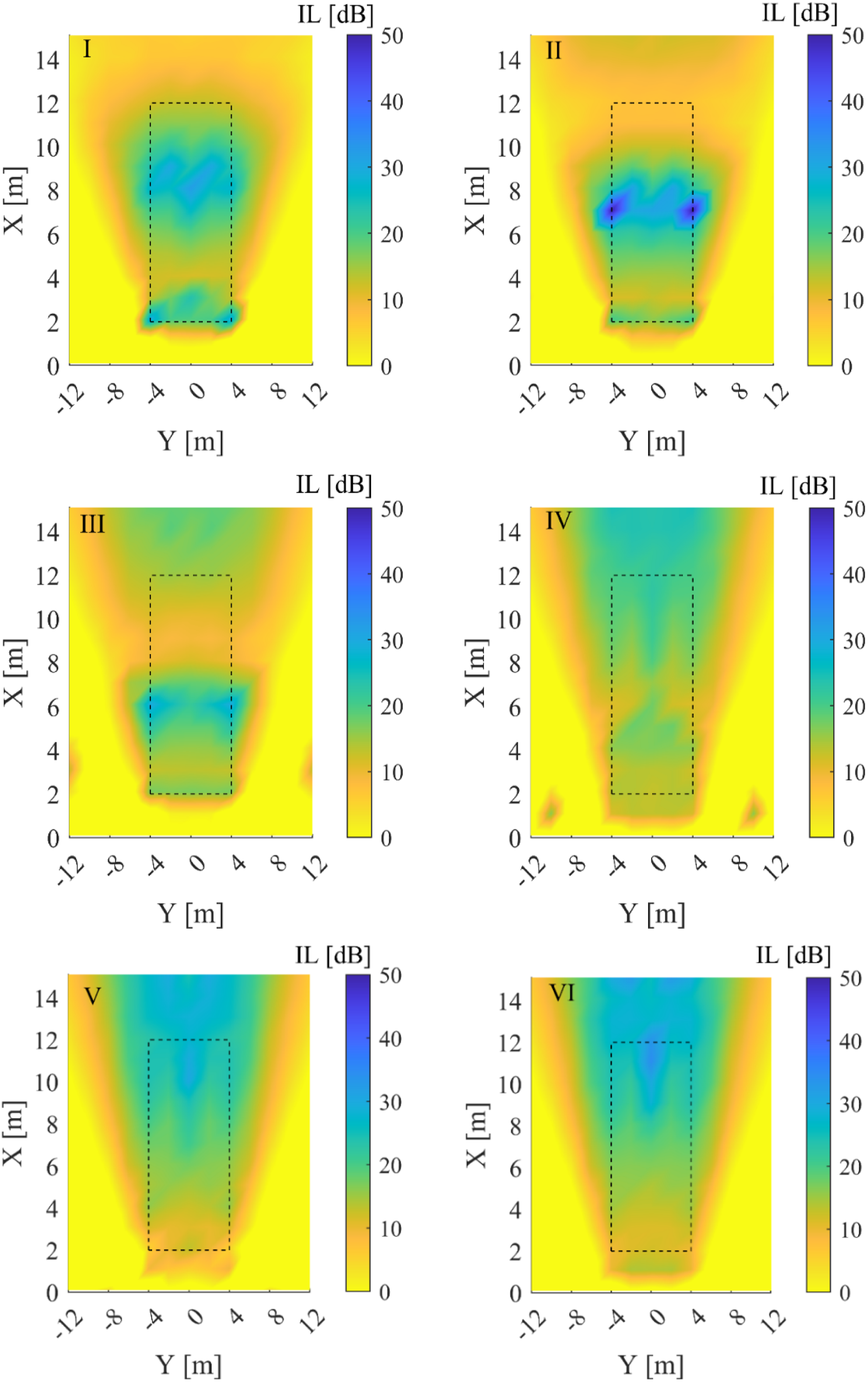

Step 2: Square pressure minimization at error microphones

The calculation of control source strength in Step 2 involves using error microphones. Research has shown that an increase in the number of error sensors can lead to greater attenuation in the target zone. However, this effect becomes negligible beyond a certain limit of error sensors.⁴⁰ To determine the upper limit of error sensors, a preliminary calculation is performed to compute the insertion loss at the target zone using $N_{s} = 3$ and $N_{s} = 4$ , with varying numbers of error microphones up to $N_{e} = 10$ (refer to Figure 5).

Figure 5.

Average insertion loss with different numbers of error microphones.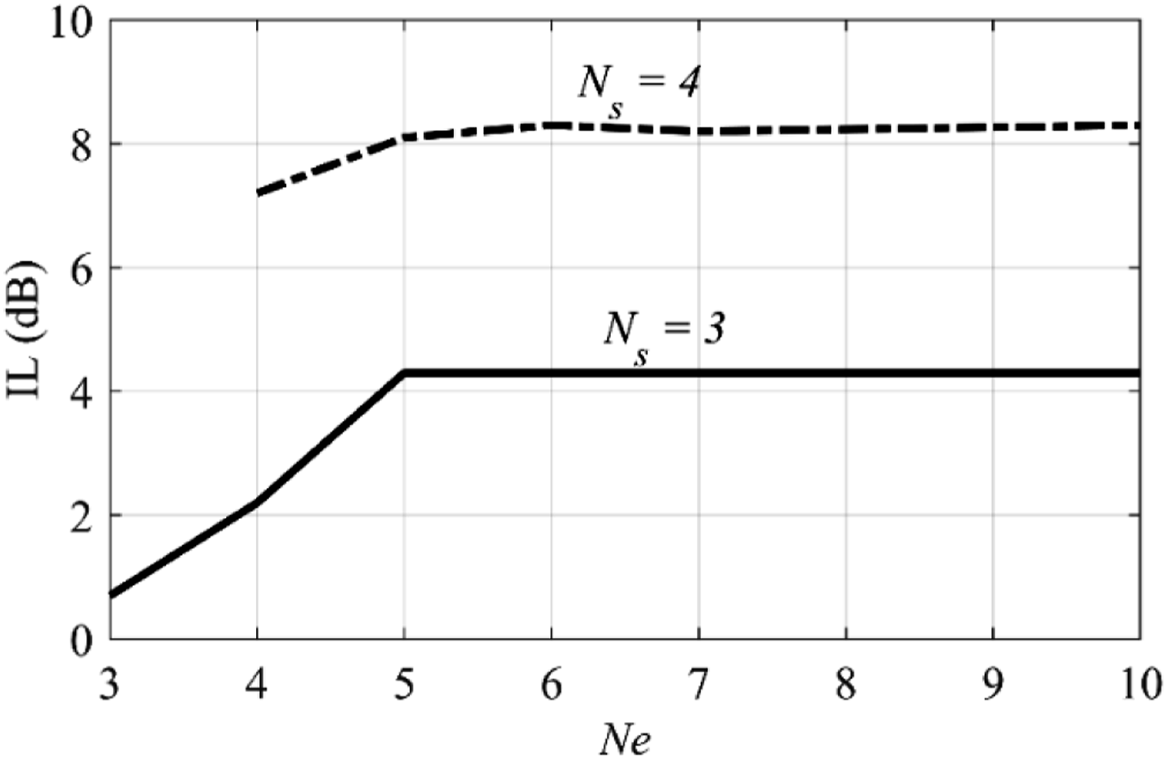

The findings indicate that in the Two-step approach increasing the number of error microphones beyond $N_{s}$ + 2 does not have a significant impact on the performance of the active noise barrier when the position of control sources is fixed. This is because, the large number of error sensors, $N_{e}$ , cover the target zone while the distance between them, $d_{e}$ , is less than the wavelength. Hence, additional error sensors will not enhance the performance of the active control system.

Therefore, further optimizations are conducted by varying the number of error microphones from

N_{e} = N_{s}

N_{e} = N_{s} + 2

. The best results of these calculations are presented in Table 4.

Table 4.

Optimized parameters of error microphones obtained by the Two-step approach at 200 Hz.

$N_{s}$	2	3	4	5	6	7	8	9	10
$N_{e}$ [m]	2	5	5	5	7	8	10	10	10
${E S}_{z}$ [m]	2.3	2.4	0.8	2.5	2.5	2.3	2.4	1.1	1.1
${E S}_{x}$ [m]	0.3	0.5	0.5	0.5	0.5	0.5	0.5	0.5	0.5
$d_{e}$ [m]	1.2	1.5	1.5	1.6	1.1	1.0	0.7	0.8	0.8
${I L}_{S t e p 2}$ [dB]	3.1	4.3	8.1	8.4	8.1	12.5	10.3	15.7	16.7
Time_{Step 2} [h]	1.9	3.0	3.7	5.4	9.1	10.4	12.0	13.3	14.5

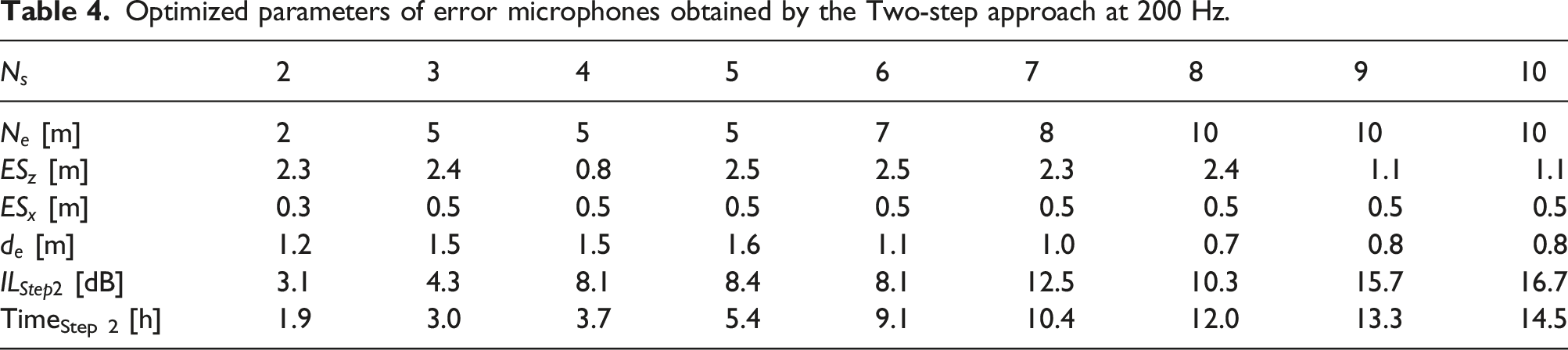
The comparison of Tables 3 and 4 clearly demonstrates that canceling the pressure at observation points leads to a higher average insertion loss than a setup with error microphones located far from the target zone, which is a predictable outcome. Table 4 reveals that there is no apparent pattern regarding the optimized locations of error microphones, but they should be situated as far away from the barrier surface as possible, similar to the results obtained for the control sources. Furthermore, the GA algorithm found that when the control sources are close to the ground, the optimal positions of error microphones are placed at heights close to the top edge. It is because when the secondary sources are close to the ground, the cancellation of the pressure at error sensors placed far from the edge would require higher control sound power. This amplification is due to the expansion of the distance between transducers and, above that, due to the increase of the diffraction angle. Probably, this amplification of acoustic power would lead to higher noise pressure levels in the target area that is far from the error sensors.

Conversely, when the control sources are situated near the top edge, the GA algorithm determined the optimal positions of error microphones at a height close to 1.0 m.

Figure 6 shows the distributions of insertion losses with 10 control sources, using the positions identified in Table 3 for Step 1 and the positions presented in Table 4 for error microphones.

Figure 6.

(Color online) IL [dB] distribution at various Zheights in the barrier’s shadow zone using the optimized configuration of the Two-Step approach for 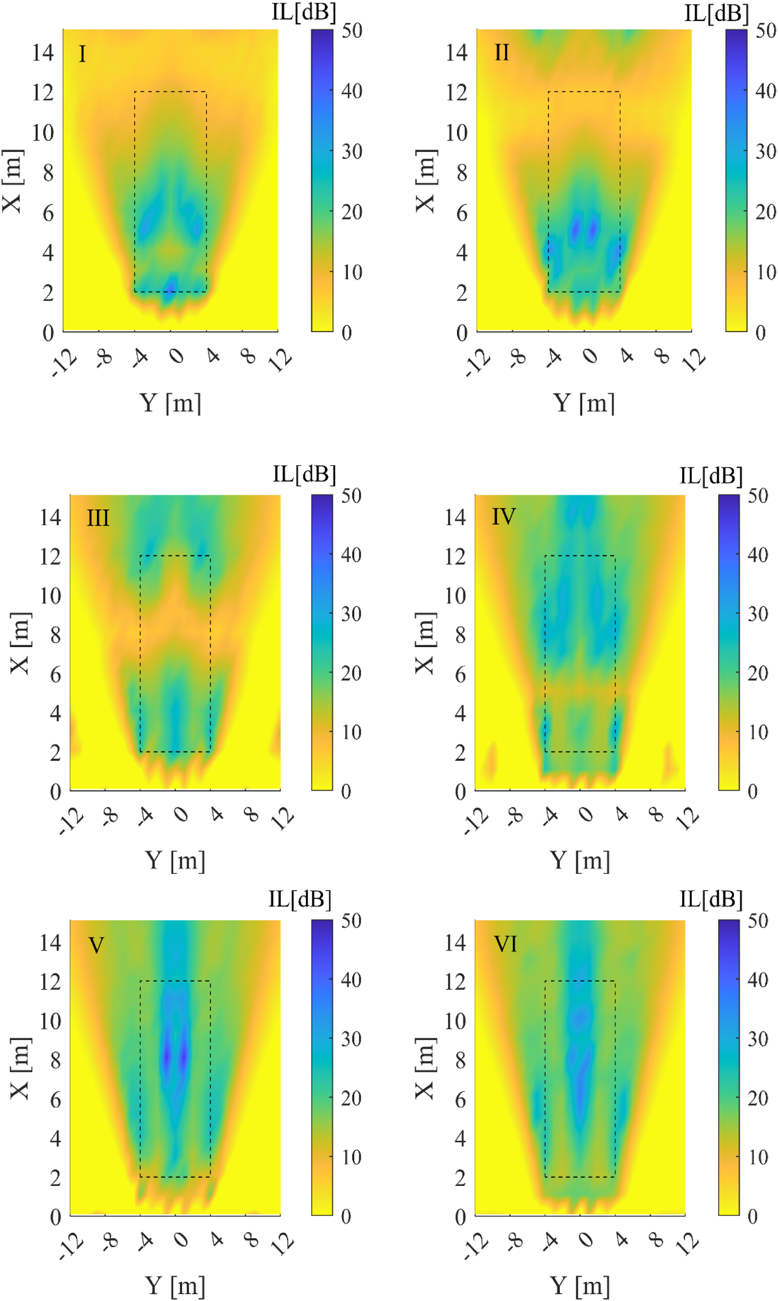$N_{s} = 10$ . Heights include (I): 2.5 m, (II): 2.0 m, (III): 1.5 m, (IV): 1.0 m, (V): 0.5 m, (VI): ground level. The rectangular dash illustrates the projection of the target area on each plane. (Print in color).

The distribution of insertion loss in Step 2, as shown in Figure 6, follows the same pattern as in Step 1 (Figure 4). The lower the height of observational points, the greater the attenuation achieve. However, the presence of error microphones has resulted in some irregular attenuation patterns close to the barrier. In Figure 4, the attenuation was mostly concentrated around the projection of the target area. On the other hand, optimizing the positions of error microphones, as illustrated in Figure 6, has led to higher noise reduction near the barrier.

Optimization with the multi-parameter approach

In this approach, the optimizations are carried out by taking into account all the parameters related to the positions of control sources and error sensors positions,

{S S}_{x}

{S S}_{z}

d_{s}, N_{e}, {E S}_{x}

{E S}_{z}

, and

d_{e}

, except for the number of control sources, which has remained constant in each calculation based on the criteria of Step 1 of the Two-step approach. The boundary limits for these parameters are the same as those presented in Table 1, and

N_{e}

should be less than

N_{s} + 2

, as previously demonstrated. Table 5 shows the optimal positions found for the transducers using the multi-parameter approach.

Table 5.

Optimal variable values of using the Multi-parameter approach at 200 Hz.

$N_{s}$	2	3	4	5	6	7	8	9	10
${S S}_{z}$ [m]	0.5	0	2.4	0.1	0.8	2.2	1.3	2.4	2.4
${S S}_{x}$ [m]	−0.5	−0.5	−0.5	−0.5	−0.5	−0.5	−0.4	−0.4	−0.5
$d_{s}$ [m]	1.5	1.0	1.3	0.9	1.1	0.5	1.1	0.8	0.7
$N_{e}$ [m]	2	5	6	7	6	9	10	11	10
${E S}_{z}$ [m]	1.4	2.4	0.7	2.3	2.3	0.4	0.2	1.0	1.1
${E S}_{x}$ [m]	0.1	0.5	0.3	0.5	0.4	0.5	0.2	0.4	0.5
$d_{e}$ [m]	0.9	1.5	0.9	1.0	1.0	0.9	1.1	0.8	0.9
$I L$ [dB]	3.1	4.3	8.0	9.5	10.3	12.9	13.0	16.7	16.9
Time [h]	1.8	2.4	2.8	3.6	5.3	6.8	8.0	9.4	11.3

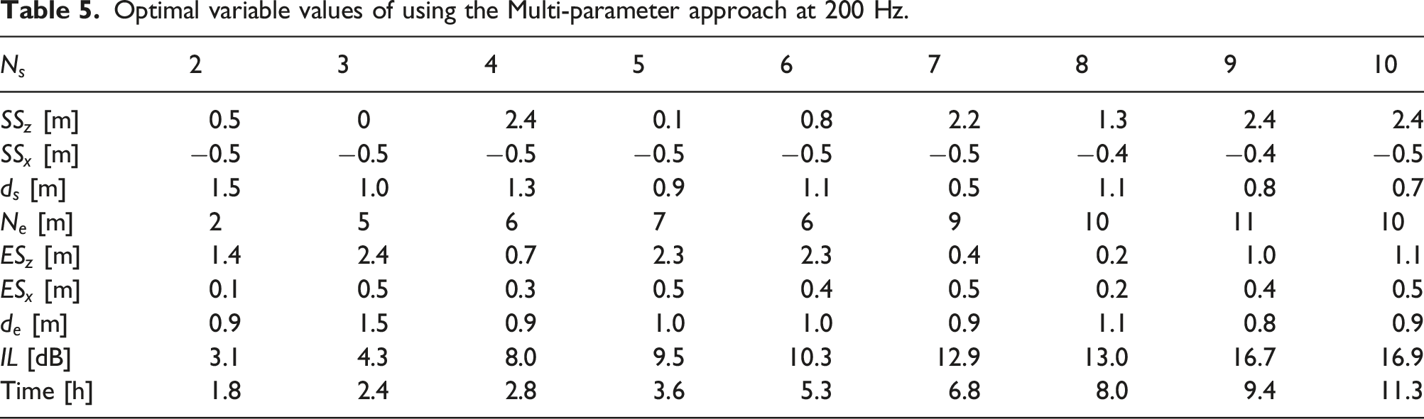
The GA optimization results for all of these parameters are presented in Table 5.

Table 5 reveals that the optimal positions for the secondary sources differ from those obtained through the Two-step approach (as shown in Tables 3 and 4). This indicates that even for the same target area, the positions that yield the best noise cancellation directly at the target area may not align with those obtained when the noise is canceled at the error microphones. However, the optimum X-coordinates of control sources ( ${S S}_{x}$ ) are typically farthest from the barrier’s surface, while the error microphones are distributed opposingly in the vertical plane, that is, when the control sources are positioned at high, the error microphones are positioned down, and vice versa.

Moreover, the Multi-parameter approach generally achieves higher attenuation than the Two-Step approach. This suggests that optimizing all parameters simultaneously can result in better performance, especially as the number of control sources increases. Additionally, due to the fewer number of generations required for the optimization process, the Multi-parameter technique demands less computational effort than the Two-step approach.

The reason for this improvement is that the Multi-parameter approach seeks the best configuration for the combination of sources and error sensors simultaneously in which it provides the maximum attenuation at the target zone. However, in the first step of the Two-step approach, the best location for control sources is searched in order to reduce the sound field across the “entire target zone,” without considering the error sensors in the calculation. Afterward, in the second step, the location of the control sources is blocked (fixed) and only the best position of the error sensors is found. Since the control sources are not optimally located with respect to the overall setup, the attenuation achieved by this method is lower than that of the multi-parameter approach.

The results also demonstrate that a control system with a few secondary sources can effectively suppress noise when the intervals between them are less than the wavelength ( $d_{s} < λ$ ), consistent with the results obtained through the Two-step calculations and supported by previous studies.^9,39 Furthermore, optimizing all parameters simultaneously results in a greater distance between control sources, $d_{s}$ , compared to directly canceling the noise at the observation points (Table 3).

Additionally, when $d_{e}$ is less than or approximately equal to half of the wavelength ( $\frac{λ}{2}$ ), increasing the number of error microphones does not significantly enhance the performance of the active control system. Figure 7 presents the distribution of insertion loss with transducers located at the optimal positions presented in Table 5 for $N_{s} = 10$ .

Figure 7.

(Color online) IL [dB] distribution at various Z heights in the barrier’s shadow zone using the optimized configuration of the Multi-parameter approach for 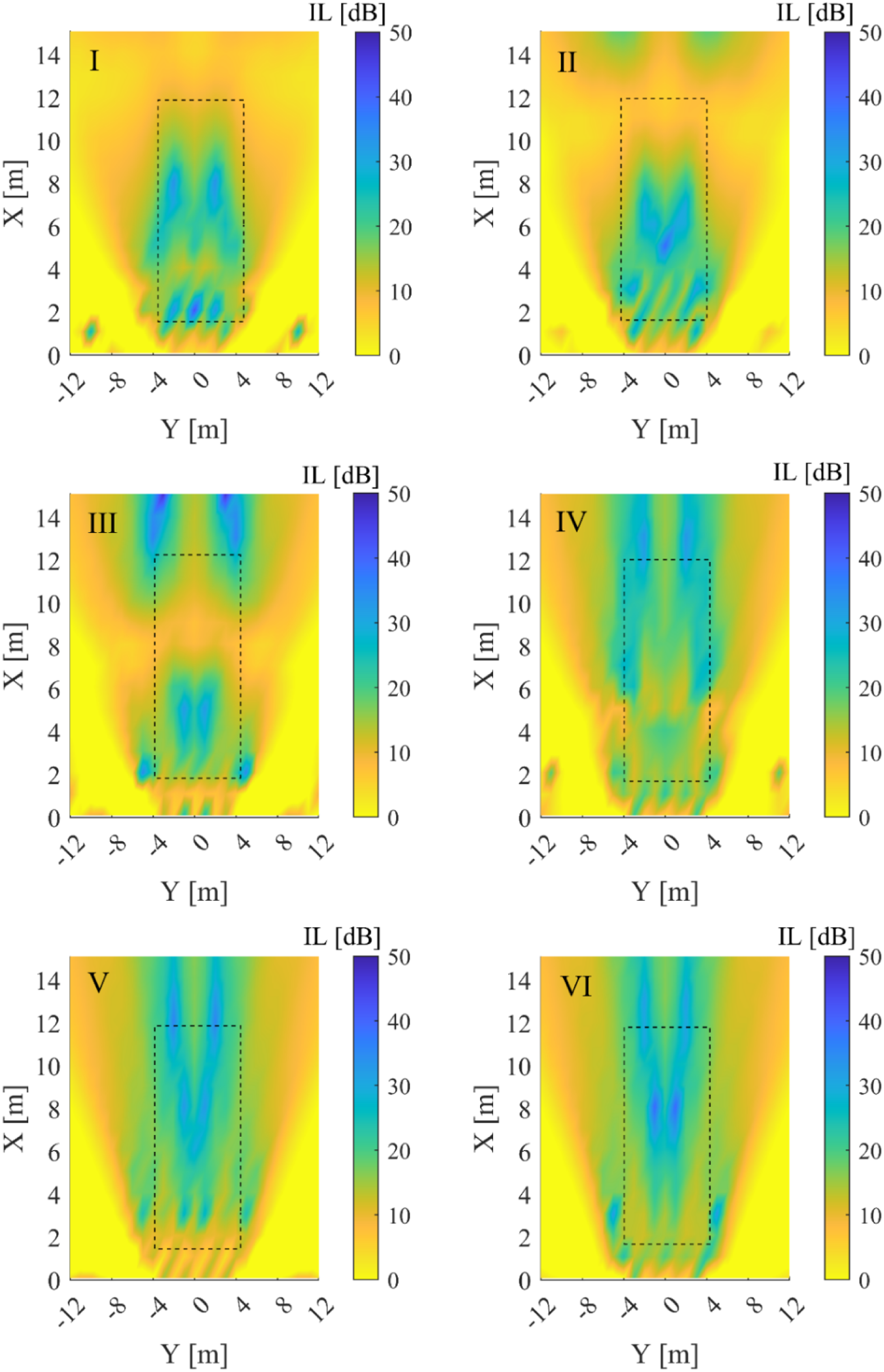$N_{s} = 10$ . Heights include (I): 2.5 m, (II): 2.0 m, (III): 1.5 m, (IV): 1.0 m, (V): 0.5 m, (VI): ground level. Rectangular dash illustrates the projection of the target area on each plane. (Print in color).

Figure 7, depicting the distribution of insertion loss with the Multi-parameter approach, indicates an increase in attenuation in a particular area of the shadow zone near the barrier, compared to the two-step approach (Figure 6). However, this improvement is not consistent throughout the entire volume of the shadow zone.

Additionally, the calculations show that the strengths of the control sources are symmetrical. In fact, when the target zone, location of transducers, and placement of the primary source are symmetrical with respect to an axis the computation of half of the vector of control sources' strength is sufficient. This simplification reduces the computational effort required, particularly when numerous iterations are necessary for the optimization process.

Optimization of the spacing between adjacent control sources and error microphones

Previous studies^8,10,11,41 have employed a uniform distribution of transducers with constant spacing between adjacent control sources or error sensors for each transducer pair. While this uniform distribution is suitable for canceling a primary plane wave,^39,42 it may not be optimal for a primary source that is relatively close to the barrier as the wavefronts are not plane waves, and the apparent distance between secondary sources in the direction of the wavefront is not the same for each pair of sources.

To address this issue and examine the effect of wavefront curvature on the active control system’s performance, the Multi-parameter approach is used to define the optimal distances between control sources and error microphones for four cases with $N_{s} = 7$ , $8$ , $9$ , and $10 .$ For each case, the number of error microphones are varied from $N_{e} = N_{s}$ to $N_{e} = N_{s} + 2$ .

Figure 8 provides a schematic presentation of control sources and error microphones with unequal spacing. However, these sources and microphones are always symmetrical with respect to the X-axis, taking advantage of the secondary strengths' symmetry found in previous sections.

Figure 8.

Various spacings between adjacent control sources and error microphones.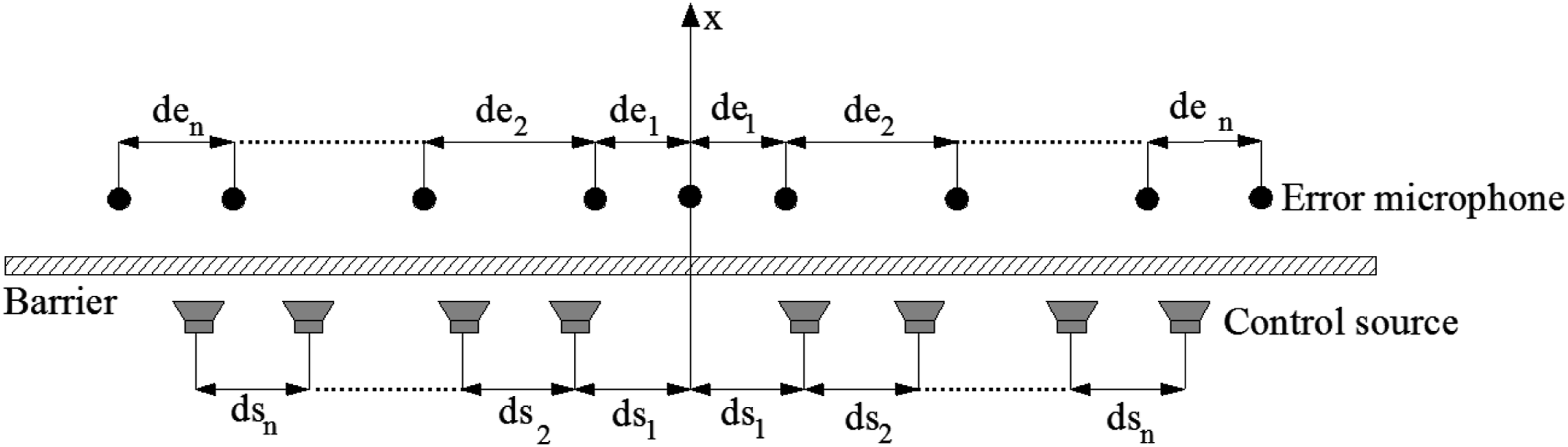

Table 6 presents the optimized distances, the transducer locations, and attenuations at the target zone.

Table 6.

Optimized parameters for control sources and error microphones.

$N_{s}$	$7$	8	9	10
${S S}_{z}$	2.4	2.4	2.5	2.5
${S S}_{x}$	−0.5	−0.5	−0.5	−0.5
${d s}_{1}$	1.5	0.3	0.6	0.3
${d s}_{2}$	1.1	1.3	1.4	0.6
${d s}_{3}$	0.5	1.0	0.4	0.5
${d s}_{4}$	—	0.3	0.5	1.2
${d s}_{5}$	—	—	—	0.3
$N_{e}$	9	8	10	10
${E S}_{z}$	1.1	0.4	0.4	0.4
${E S}_{x}$	0.4	0.5	0.5	0.4
${d e}_{1}$	0.5	0.6	0.5	0.4
${d e}_{2}$	1.5	0.5	1.1	0.5
${d e}_{3}$	1.2	1.3	0.7	1.4
${d e}_{4}$	0.3	1.2	1.0	0.9
${d e}_{5}$	—	—	0.4	0.6
IL [dB]	19.5	18.2	19.5	19.1

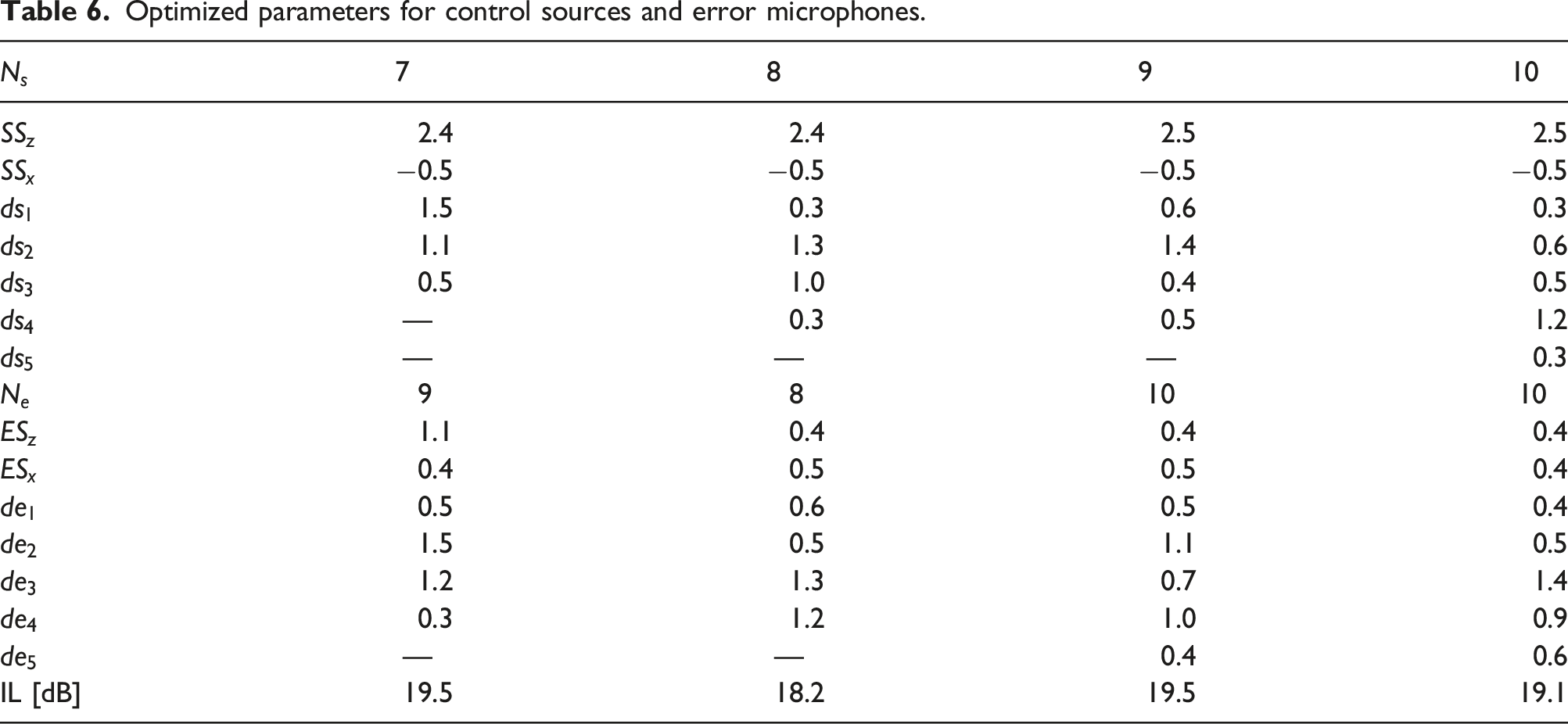
By comparing Tables 5 and 6, it can be observed that the optimal positions for the transducers follow the same trend as the previous, that is, the control sources and error microphones are far from the barrier and oppositely distributed along with the vertical distance. Additionally, as presented in Table 6, optimizing the distances between adjacent transducers, along with other parameters, can significantly enhance the performance of the active noise control system. Moreover, the number of transducers can be significantly reduced compared to a set of evenly distributed transducers, without a loss of performance.

Figure 9 displays the distribution of insertion loss in the shadow zone at varying heights with 10 control sources and 10 error microphones which are placed according to Table 6.

Figure 9.

(Color online) IL [dB] distribution at various Z heights in the barrier’s shadow zone using the optimized 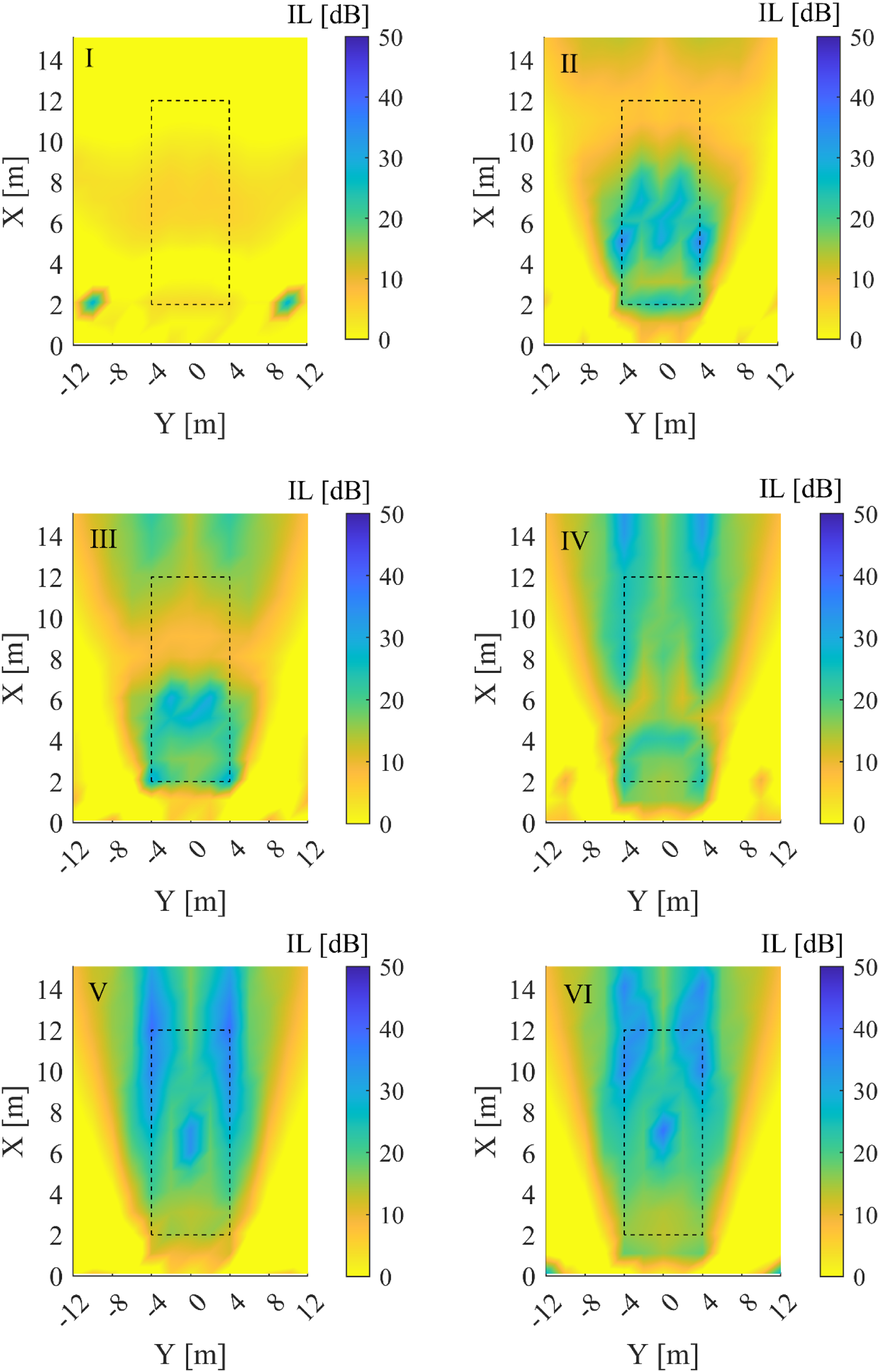$d s$ and $d e$ and $d e$ distances for $N_{s} = N_{e} = 10$ . Heights include (I): 2.5 m, (II): 2.0 m, (III): 1.5 m, (IV): 1.0 m, (V): 0.5 m, (VI): ground level. The rectangular dash illustrates the projection of the target area on each plane. (Print in color).

Figure 9 shows that optimizing the spacing between control sources and error sensors results in a concentration of attenuations within the target area and below it. Moreover, utilizing variable distances leads to a more uniform attenuation in these regions.

Conclusions

In this study, the optimal placement of transducers for an active noise barrier was determined using the genetic algorithm optimizer in MATLAB. To achieve maximum attenuation, secondary sources were located on the incident side and error sensors were placed on the receiver side, both transducers positioned below the height of the barrier, as established in previous investigations. A regular distribution of the array of secondary sources or error sensors was utilized, with equal distance between adjacent transducers, but the spacing between control sources may not be the same as the spacing between error sensors.

Two approaches were employed: (1) Two-step approach, where in the first step the position of secondary sources was determined, and then in the second step the location of error sensors was optimized, and (2) Multi-parameter approach, where the position of all transducers was simultaneously calculated.

Overall, the Multi-parameter approach was found to be preferable due to the following reasons: (i) with the same number of control sources, a higher noise level reduction was obtained at the target zone (approximately 1 dB difference), (ii) noise reduction was achieved in a wider area of the shadow zone, and (iii) less computation effort was required. Moreover, for symmetrical problems, the computational effort can be further reduced by computing half of the vector of control sources’ strength.

As noted in the introduction, while there is an optimal position for transducers, previous research has shown that there are numerous configurations that may result in attenuations close to the optimal values. Considering this fact and based on the results of this study, general criteria can be established for the design of an active noise barrier:

• The distance between secondary sources or error sensors should be equal to the width of the target zone divided by the number of transducers and must not exceed the wavelength of the primary noise.

• Increasing the number of secondary sources, leads to higher attenuation, up to a certain point, where the distance between them is at half of the wavelength. After this point, the performance gain is minimal.

• The number of error sensors should be within the range of the number of secondary sources and that number increased by two units. Further increase in the number of error sensors does not improve performance.

• Transducers should be positioned below the height of the barrier and at the farthest distance from the barrier surface, but distributed oppositely. Specifically, when the control sources are placed close to the top edge of the barrier, the error microphones should be positioned at lower heights, and vice versa.

Thus, by following these criteria, the active noise barrier can be optimized for a given number of secondary sources.

Additionally, when dealing with non-plane primary noise waves, using a set of transducer arrays with unequal distances between adjacent transducers can improve performance compared to using a regular array. Moreover, this optimization method can significantly reduce the number of required transducers while maintaining or even improving system performance.

Footnotes

Declaration of conflicting interests

The author(s) declared no potential conflicts of interest with respect to the research, authorship, and/or publication of this article.

Funding

The author(s) disclosed receipt of the following financial support for the research, authorship, and/or publication of this article: This work was supported by the Agència de Gestió d’Ajuts Universitaris i de Recerca (2020 FI_B2 00073).

ORCID iD

Shahin Sohrabi

References

Berkhoff

. Control strategies for active noise barriers using near-field error sensing. J Acoust Soc Am 2005; 118: 1469–1479. DOI: 10.1121/1.1992787

Hart

Lau

. Active noise control with linear control source and sensor arrays for a noise barrier. J Sound Vib 2012; 331: 15–26. DOI: 10.1016/j.jsv.2011.08.016

Sohrabi

Pamies

Romeu

. Evaluation of the effectiveness of control sources’ interval on active noise control performance. In: INTER-NOISE 2019: 48th international congress and exposition on noise control engineering, Madrid: Institute of Noise Control Engineering; 2019, p. 4196–4204.

Sohrabi

Gómez

Garbí

. Investigate the effect of the active noise barrier on the reduction of noise level at the shadow zone and the neighboring building. In: INTER-NOISE and NOISE-CON congress and conference proceedings. Seoul, Korea. Institute of Noise Control Engineering, 2020, pp. 1978–1987; 261.

Huang

Zou

Qiu

. A preliminary study on the performance of indoor active noise barriers based on 2D simulations. Build Environ 2015; 94: 891–899. DOI: 10.1016/j.buildenv.2015.06.034

Sohrabi

Pamies

Romeu

. Numerical study of an active noise barrier. In: NTER-NOISE 2017: 46th international congress and exposition on noise control engineering, Hong Kong, 27–30 August 2017, 2017-Janua:5313–21.

Sohrabi

Pamies

Romeu

. Numerical study of an active noise barrier. In: INTER-NOISE 2017 - 46th International Congress and Exposition on Noise Control Engineering, Hong Kong, China, 27-30 August 2017.

Omoto

Fujiwara

. A study of an actively controlled noise barrier. J Acoust Soc Am 1993; 94: 2173–2180. DOI: 10.1121/1.407488

Shao

Sha

Zhang

. The method of the minimum sum of squared acoustic pressures in an actively controlled noise barrier. J Sound Vib 1997; 204: 381–385. DOI: 10.1006/jsvi.1997.0909

10.

Niu

Zou

Qiu

, et al. Error sensor location optimization for active soft edge noise barrier. J Sound Vib 2007; 299: 409–417. DOI: 10.1016/j.jsv.2006.08.005

11.

Sohrabi

Pàmies Gómez

Romeu Garbí

. Suitability of active noise barriers for construction sites. Appl Sci 2020; 10: 6160. DOI: 10.3390/app10186160

12.

Sohrabi

Pàmies Gómez

Romeu Garbí

. Proper location of the transducers for an active noise barrier. J Vib Control 2022; 29. DOI: 10.1177/10775463221077490

13.

Shor

. Minimization methods for non-differentiable functions. Heidelberg, Germany: Springer Science and Business Media, 2012, 3.

14.

Fogel

. Evolutionary computation: toward a new philosophy of machine intelligence. New Jersey, United States: John Wiley and Sons, 2006, 1.

15.

Back

. Evolutionary algorithms in theory and practice: evolution strategies, evolutionary programming, genetic algorithms. New York, United States: Oxford university press, 1996.

16.

Marler

Arora

. Survey of multi-objective optimization methods for engineering. Struct Multidiscipl Optim 2004; 26: 369–395. DOI: 10.1007/s00158-003-0368-6

17.

Duhamel

. Shape optimization of noise barriers using genetic algorithms. J Sound Vib 2006; 297: 432–443. DOI: 10.1016/j.jsv.2006.04.004

18.

Baulac

Defrance

Jean

. Optimisation with genetic algorithm of the acoustic performance of T-shaped noise barriers with a reactive top surface. Appl Acoust 2006; 69: 332–342. DOI: 10.1016/j.apacoust.2006.11.002

19.

Gounot

YJR

Musafir

. Genetic algorithms: a global search tool to find optimal equivalent source sets. J Sound Vib 2009; 322: 282–298. DOI: 10.1016/j.jsv.2008.11.001

20.

Tao

Wang

Qiu

, et al. Performance of a multichannel active sound radiation control system near a reflecting surface. Appl Acoust 2017; 123: 1–8. DOI: 10.1016/j.apacoust.2017.02.020

21.

Toledo

Aznárez

Maeso

, et al. Optimization of thin noise barrier designs using evolutionary algorithms and a dual BEM formulation. J Sound Vib 2015; 334: 219–238. DOI: 10.1016/j.jsv.2014.08.032

22.

Wong

. A review of commonly used analytical and empirical formulae for predicting sound diffracted by a thin screen. Appl Acoust 2005; 66: 45–76. DOI: 10.1016/j.apacoust.2004.06.004

23.

Matsui

Takagi

Hiramatsu

, et al. Outdoor sound propagation from a source having dimensions. J Acoust Soc Japan 1989; 45. DOI: 10.20697/jasj.45.7_512

24.

Embleton

TFW

. Tutorial on sound propagation outdoors. J Acoust Soc Am 1996; 100. DOI: 10.1121/1.415879

25.

Attenborough

. Review of ground effects on outdoor sound propagation from continuous broadband sources. Appl Acoust 1988; 24: 289–319. DOI: 10.1016/0003-682X(88)90086-2

26.

Nelson

Elliott

. Active control of sound. Academic. San Diego, CA, USA: Academic Press; 1st edition (January 6, 1992), 1992.

27.

Ahmad

Khan

. Variational iteration algorithm-I with an auxiliary parameter for wave-like vibration equations. J Low Freq Noise Vib Act Control 2019; 38: 1113–1124. DOI: 10.1177/1461348418823126

28.

Ahmad

Khan

Cesarano

. Numerical solutions of coupled burgers’ equations. Axioms 2019; 8. DOI: 10.3390/axioms8040119

29.

Ahmad

Khan

Stanimirovic

, et al. Modified variational iteration technique for the numerical solution of fifth order KdV-type equations. J Appl Comput Mech 2020; 6: 1220–1227. DOI: 10.22055/JACM.2020.33305.2197

30.

Ahmad

Seadawy

Khana

. modified variational iteration algorithm to find approximate solutions of nonlinear Parabolic equation. Mathemat Comput Simul 2020; 177: 13–23.

31.

Bazighifan

Ahmad

Yao

. New oscillation criteria for advanced differential equations of fourth order. Mathematics 2020; 8. DOI: 10.3390/MATH8050728

32.

Mathworks . MATLAB global optimization toolbox. Manual. Natick, MA, USA: The MathWorks, 2016.

33.

Romeu

Palacios

Balastegui

, et al. Optimization of the active control of turboprop cabin noise. J Aircr 2015; 52: 1386–1393. DOI: 10.2514/1.C032431

34.

Palacios

Romeu

Balastegui

. Two step optimization of transducer locations in single input single output tonal global active noise control in enclosures. J Vib Acoust 2010; 132: 061011. DOI: 10.1115/1.4002122

35.

Svensson

Sohrabi

. Modeling sound transmission through apertures with diffraction. In: INTER-NOISE and NOISE-CON congress and conference proceedings. Glasgow, Scotland: Institute of Noise Control Engineering, 2023, pp. 6092–6102, 265.

36.

Liu

JCC

Niu

. Study on the analogy feedback active soft edge noise barrier. Applied Acoustics 2008; 69: 728–732. DOI: 10.1016/j.apacoust.2007.02.008

37.

Nagamatsu

Ise

Shikano

. Optimum arrangement of secondary sources and error sensors for. Active Noise Barrier 2000; 1: 2–6.

38.

Omoto

Takashima

Fujiwara

, et al. Active suppression of sound diffracted by a barrier: an outdoor experiment. J Acoust Soc Am 1997; 102: 1671–1679. DOI: 10.1121/1.420078

39.

Elliott

Cheer

Bhan

, et al. A wavenumber approach to analysing the active control of plane waves with arrays of secondary sources. J Sound Vib 2018; 419: 405–419. DOI: 10.1016/j.jsv.2018.01.028

40.

Romeu

Balastegui

Pàmies

, et al. Optimal acoustic error sensing for global active control in a harmonically excited enclosure. Acoust Phys 2014; 60: 77–85. DOI: 10.1134/S1063771014010114

41.

Chen

Rao

Min

, et al. An active noise barrier with unidirectional secondary sources. Appl Acoust 2011; 72: 969–974. DOI: 10.1016/j.apacoust.2011.06.006

42.

Lam

Shi

, et al. Active control of sound through full-sized open windows. Build Environ 2018; 141: 16–27. DOI: 10.1016/j.buildenv.2018.05.042

Using genetic algorithms to optimize the location of transducers for an active noise barrier

Abstract

Keywords

Introduction

Theory

Diffraction model

Minimization of square pressure at error microphones

Average insertion loss in an area

Methodology

Model description

Optimization approaches

Two-step approach

Multi-parameter approach

Results and discussions

Model validation

Optimization with the two-step approach

Step 1: Square pressure minimization at the observation points

Step 2: Square pressure minimization at error microphones

Optimization with the multi-parameter approach

Optimization of the spacing between adjacent control sources and error microphones

Conclusions

Footnotes

Declaration of conflicting interests

Funding

ORCID iD

References