
Abstract
In this paper, we study a stochastic SIS epidemic model with distributed delays. The positiveness of the solutions is established. We obtain sufficient conditions for the extinction of the disease through the study of stochastic stability of the disease-free equilibrium and stability of the same equilibrium in the mean. Compared to many works on the deterministic and stochastic SIS models and their stability, the distributed delays involved in the model offer new conditions with much more boundedness on the rate of losing immunity. The disease is extinct for small and large enough values of the intensity of noise and regardless of the initial history functions and the magnitude of the basic reproductive number R0.
Keywords
Introduction
Many authors have investigated the dynamic behaviors of the SIVS model. Numerous studies have drawn inspiration from continuous and pulse vaccination strategies in mathematical epidemiology.1–4 These studies have explored the relationship between the basic reproduction number R0 and the persistence or extinction of the disease. The disease dies out and if R0 > 1, the disease persists. A vaccinated individuals compartment has been added to the mathematical model with a rate of losing immunity.5–8
For a more realistic mathematical model, we formulate the SIS epidemic model with distributed time delays. This formulation assumes that the delay is a distributed parameter within the interval [0, τ], where τ represents the upper limit of the delay in time. With existing the loss of immunity rate, the deterministic SIS model with distributed delays will be in the following form
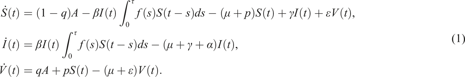
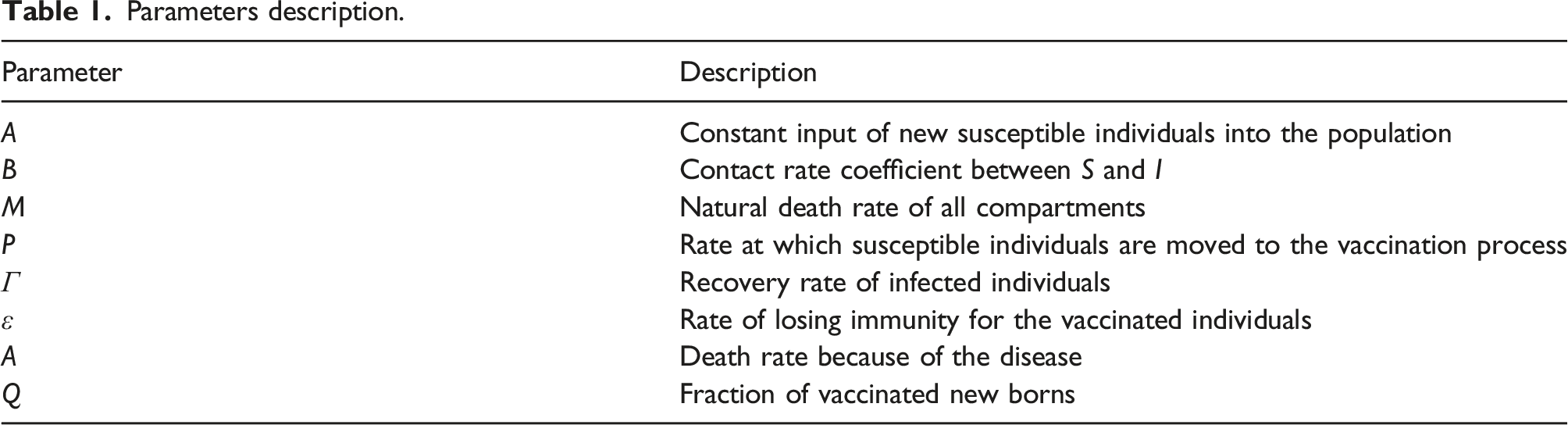
The first compartment is the susceptible individuals S(t) who are not infected until they come into contact with the second compartment, namely, infected individuals I(t). To account for the vaccination program, we introduce the compartment of vaccinated individuals V(t), who have undergone the vaccination process and acquired immunity. It is crucial to consider whether vaccinated individuals may lose their immunity over time or not. Thus, we take into consideration the rate of immunity loss, denoted as ɛ, and its impact on the disease’s extinction and persistence. It’s important to note that the specific flow and progression of an epidemic can vary depending on the disease, its characteristics, and the measures implemented to control it. The flow map in Figure 1 of the SIS epidemic visually represents the spread and progression of a disease through various stages. It illustrates the flow of infected individuals from one stage to another. The flow map of the delayed SIS model with a rate of force infection Parameters description.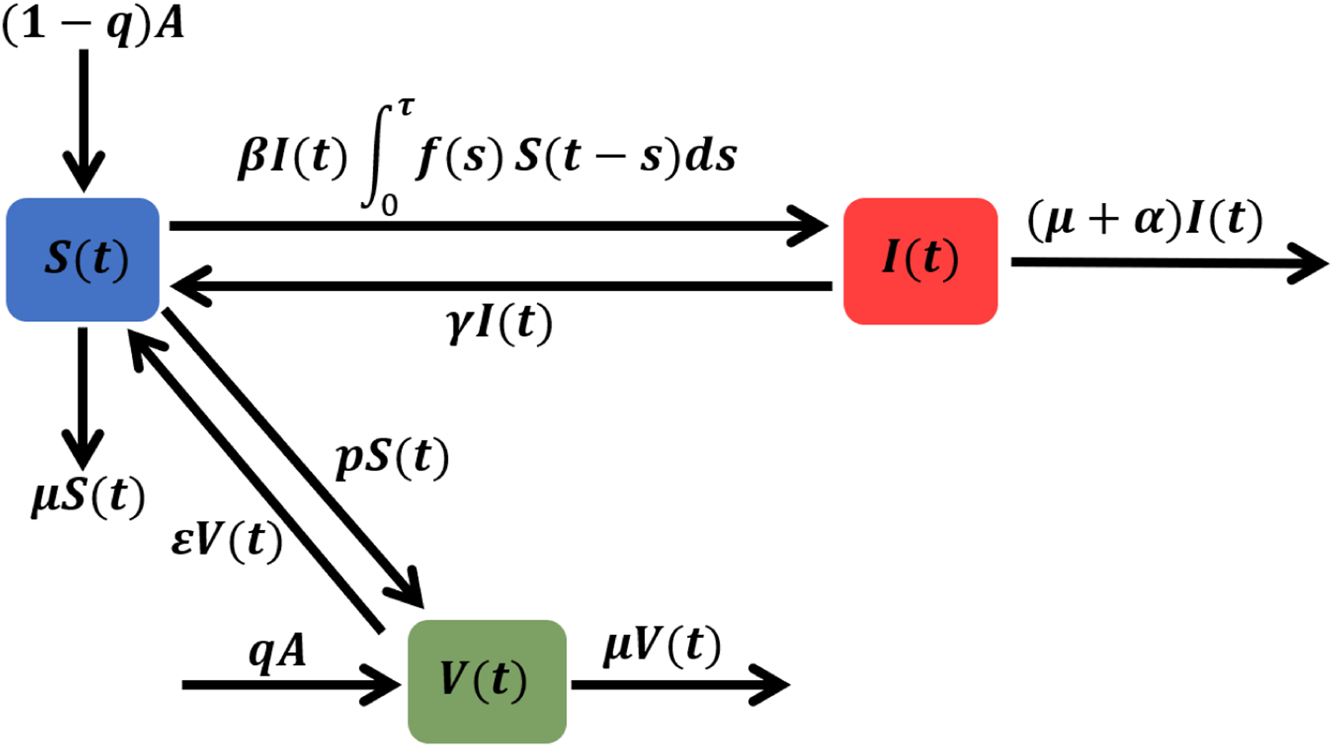
In model (1), f(s) is a non-negative square-integrable and continuous function over the interval 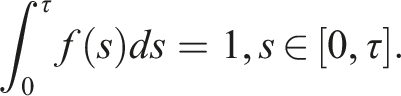
The term 
Following Ref. [9], we consider ϕ
i
(θ) ≥ 0 ∀i = 1, …, 3. All solutions of (1) are in 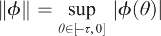
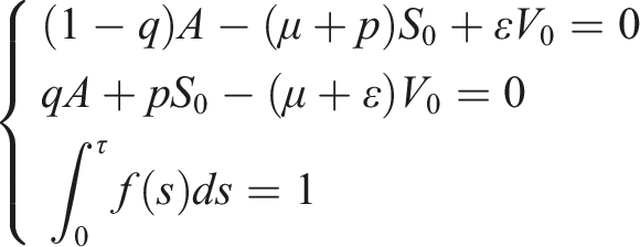
According to Ref. [10], the disease-free equilibrium of (1) is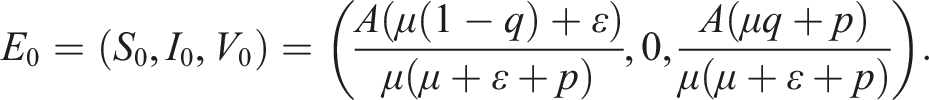
By Ref. [11], the threshold quantity of this system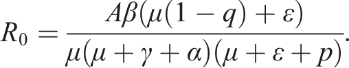
In 
To enhance disease control measures, we introduce stochastic environmental noises to perturb the deterministic system. Stochastic systems effectively capture all forms of uncertainty in dynamic behaviors. Numerous studies have focused on stochastic models and their stability, including the SIS epidemic model.12–16 Some stochastic models with discrete delays and distributed delays in time have been studied in Refs [17–19]. We employ the parametric stochastic perturbation technique,
14
utilizing the contact parameter β, to further investigate the effects of stochasticity. The stochastic epidemic model with distributed delays is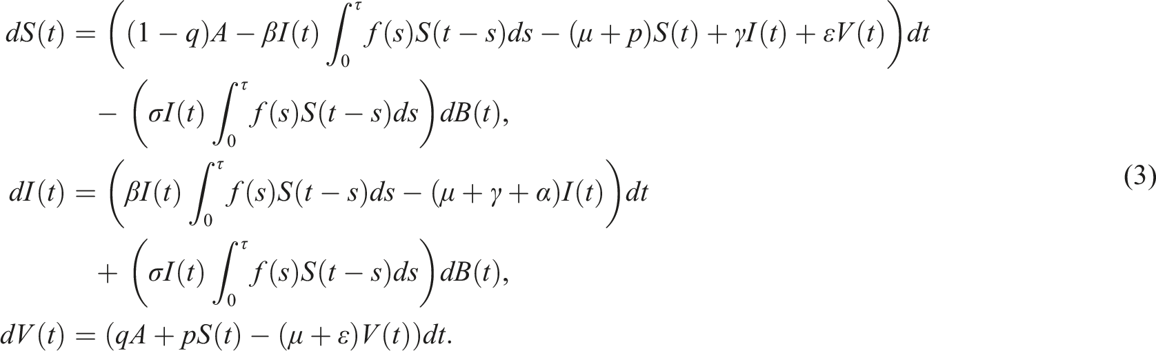
We specifically focus on examining the disease’s extinction by analyzing the stability of the disease-free equilibrium E0 through two different approaches. First, we investigate the stability in probability of E0 by centering the nonlinear system around E0 and linearizing it. Regardless of the magnitude of the basic reproduction number R0, we observe a stable disease-free equilibrium. In other words, the disease is expected to go extinct for both small and large values of the noise parameter. Additionally, we propose a boundedness condition for the immunity rate. Second, we analyze the stability of E0 in the mean. In both approaches, we introduce appropriate Lyapunov functionals to facilitate the investigation of equilibrium states’ stability within the epidemiological system.
Fractal-fractional differential equations have been widely employed to model complex phenomena such as biological systems, electrical circuits, and diffusion processes, highlighting the significance of stochasticity in these models. In Ref. [20], the authors presented a novel model employing a stochastic process to capture the impact of nonlinear perturbations and arbitrary-order derivatives. This model effectively utilizes white noises to represent and incorporate these elements into the system. This idea lays a robust groundwork for exploring analogous illnesses, carrying profound implications in the field of biological sciences. Furthermore, it holds significant relevance for investigating communicable infections like HIV and COVID-19. Numerous contemporary methods have been developed to obtain explicit solutions for both deterministic and stochastic equations, see Refs [21–26].
Although the deterministic and stochastic SIS epidemic models have been extensively studied in the literature. The incorporation of randomness and uncertainty in the epidemic model through the stochastic version enhances its realism compared to the deterministic model that has been analyzed previously by Refs [6,7,10]. While the authors in Refs [8,12,13,27] included a vaccination process in their stochastic SIS model, they did not incorporate time delays, which are necessary for modeling vaccination. To create a more realistic model, we consider the inclusion of distributed delay. Previous studies on stochastic SIS models have given limited consideration to distributed continuous time delay.28,29 Instead, they have mainly focused on determining sufficient conditions for disease extinction and permanence, but with constraints on the basic reproduction number and noise in L1. Our research introduces two significant types of stability—stochastic stability via stability in L2 space and stability in the mean—which have not been explored before. The stability in the mean ensures long-term disease extinction, even if the deterministic system is endemic. Additionally, the disease-free equilibrium remains stable in the stochastic system, regardless of the values of R0 and noise.
This work makes several novel contributions to the field. First, we propose a distributed delay in the model, which is more realistic for modeling epidemics. Distributed delays capture the time delay between infection and transmission. There is a delay between infection and transmission that varies depending on the individual and the specific disease. Distributed delays account for this variation by modeling the time delay as a distribution rather than a fixed value. This approach allows for more flexibility in modeling the complex dynamics of an epidemic, as the time delay can vary depending on the specific situation. This feature has not been previously incorporated in other studies for such SIS model. Second, the authors introduce two types of stability, stochastic stability, and stability in the mean, which have not been explored in detail by previous research. Stability in probability is proved through mean square stability that guarantees that the fluctuations around the steady state are limited and will eventually die out. Stability in the mean guarantees that the average number of individuals who become infected with a disease over time does not change significantly. Moreover, the study’s conditions ensure the stability of the model for increased levels of noise, even when the deterministic system is endemic. This result is particularly noteworthy as it highlights the robustness of the proposed model in the presence of high levels of noise.
Preliminaries and notations
Unless otherwise specified, let 
This equation arises in modeling many real-life problems, for example, see Refs [30, 31]. For 
Assume that for every initial condition x0, there exists a unique global solution such that
Denote
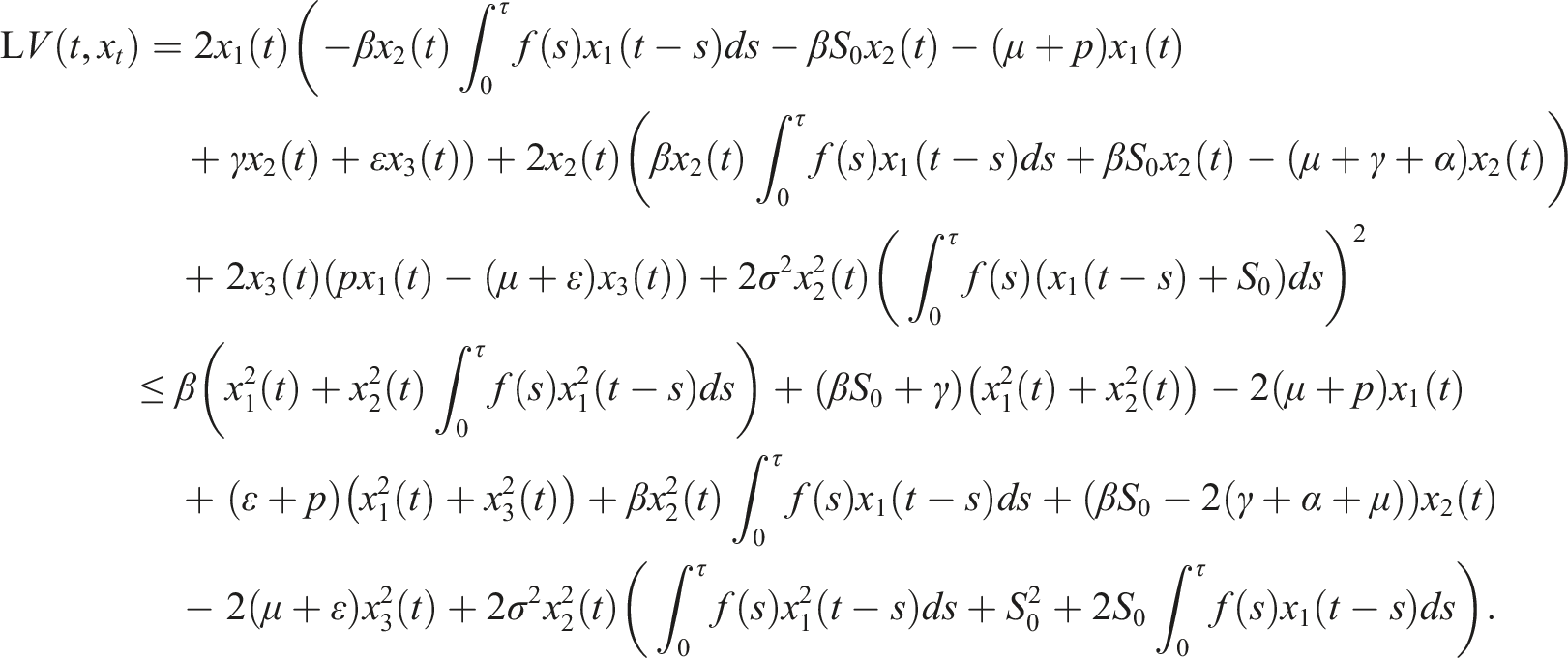
The differential operator L for all V ∈ D is given by
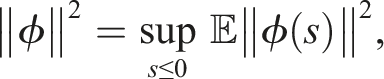
32,33 The zero solution of (4) is 1. Stochastically stable (stable in probability) if for ɛ ∈ (0, 1), ℓ > 0, ∃ δ = δ(ɛ, ℓ) > 0 and ‖ϕ‖ < δ such that 2. Mean square stable if for each ɛ > 0, ∃ δ > 0 and ‖ϕ‖2 < δ such that 3. Asymptotically mean square stable if it is mean square stable and The stability of the trivial equilibrium of (4) is discussed in the following theorems
33
Assume 1. 2. 3.
where c
i
> 0, i = 1, 2, 3, then the trivial equilibrium of (4) is asymptotically mean square stable.
33
Assume 1. V(t, x
t
) ≥ c1|x(t)|2 2. 3. LV(t, x
t
) ≤ 0 If
where c
i
> 0, i = 1, 2, 3, then the trivial equilibrium of (4) is stochastically stable.
32
A right continuous adapted process 
Well-posedness
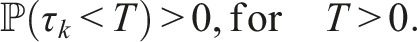
From a biological perspective, we aim to demonstrate that the solutions to (3) exist uniquely and remain positive within Ω, irrespective of the initial history functions. However, due to the coefficients of this system satisfying the local Lipschitz condition but not the linear growth condition, 32 the solution of the system is susceptible to a finite-time explosion. Therefore, we establish both the positivity and boundedness of the solution to (3) for t ≥ 0.
For any initial state
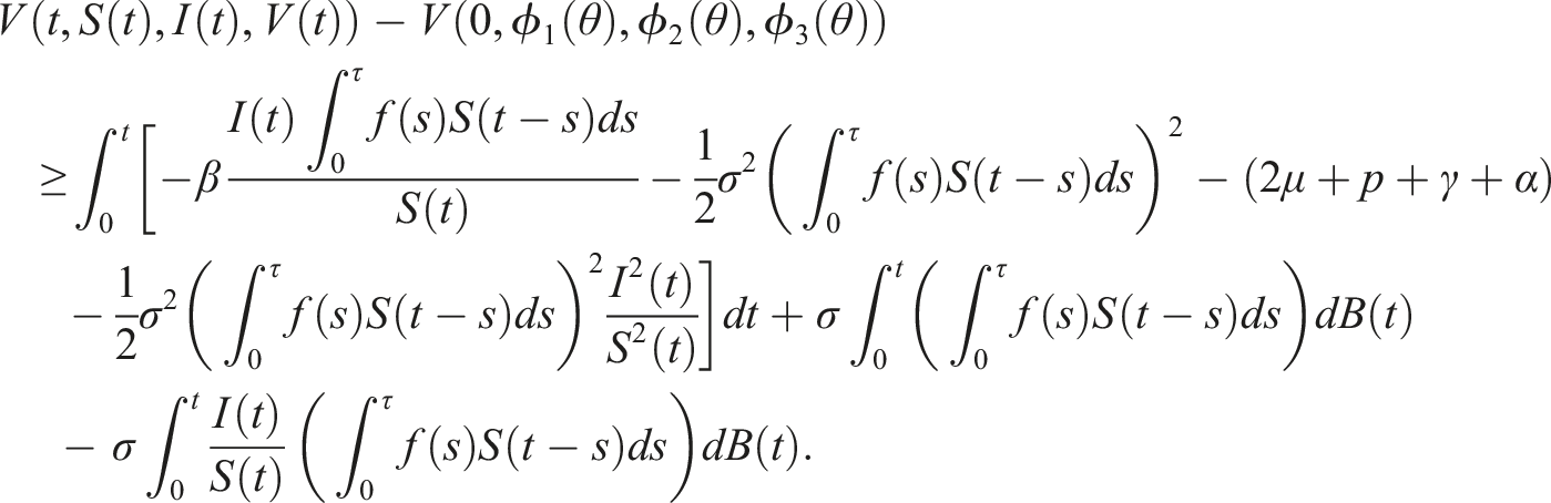
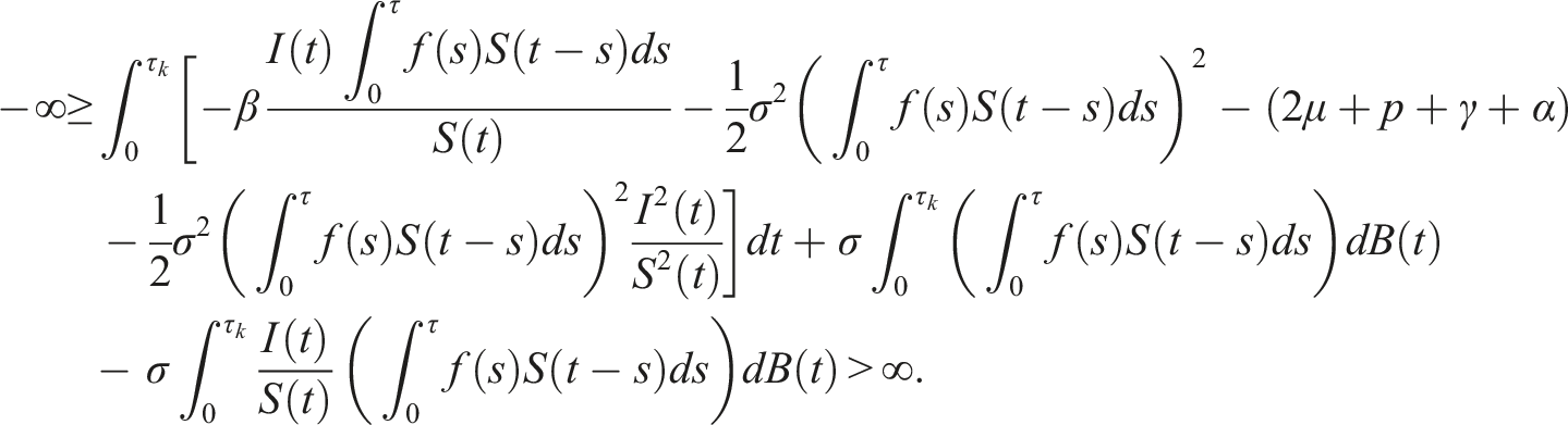
Following Refs [32, 34], the initial state Define the stopping time So, there exists k ≥ k1 such that Consider the Lyapunov functional V(t, S(t), I(t), V(t)) = ln S(t) + ln V(t), using the differential operator L in (5), we get Then The solution of (3) is positive in The contradiction arises here, so τ
k
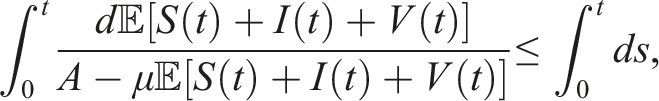
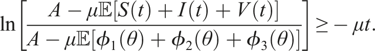
= ∞. Hence, the solution is unique, global, and remains in Now, according to (3), we have Consequently Then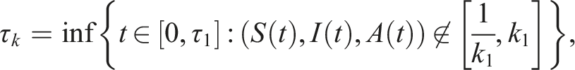


Extinction
In this section, we investigate the conditions for the extinction of the disease. We study the stochastic stability of the disease-free equilibrium and its stability in the mean. The distributed delay terms involved in the models offer sufficient conditions for the extinction of the disease.
Stability in probability
Mean square stability conditions of the trivial equilibrium of the linear system are sufficient conditions of stochastic stability of the equilibrium states of the corresponding nonlinear system. This is our approach to the study of the stability of E0. We obtain sufficient conditions for stochastic stability of E0 with some restrictions on the rate of losing immunity. Also, these conditions ensure the eradication of the disease, even if the basic reproduction number R0 is greater than 1. This is possible due to the presence of noise, which helps stabilize the system and prevent the disease from spreading. The following lemma gives sufficient conditions for mean square stability of the corresponding linear system of (3).
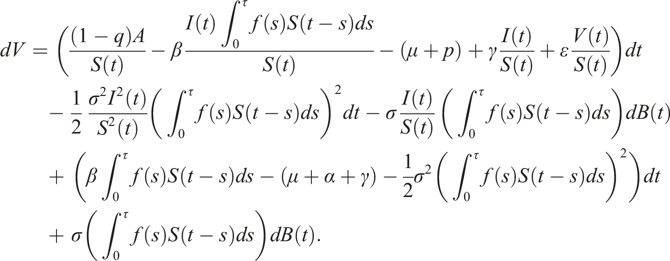
Let us center (3) at the disease-free equilibrium E0 = (S0, I0, V0) using the transformations
By this way, we obtain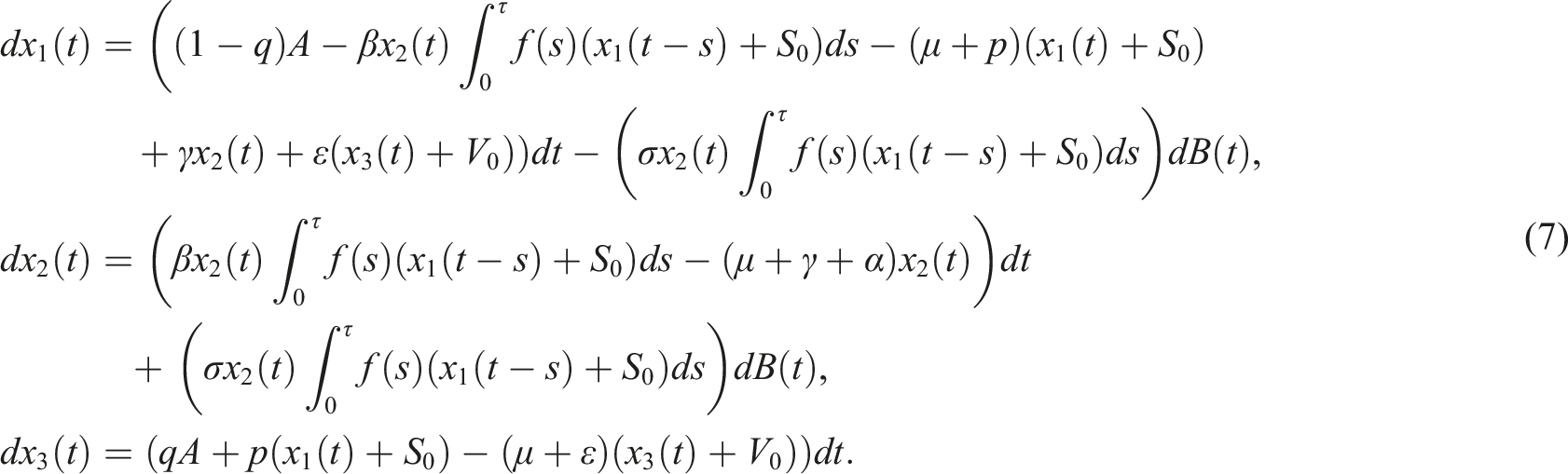
And the corresponding linear system is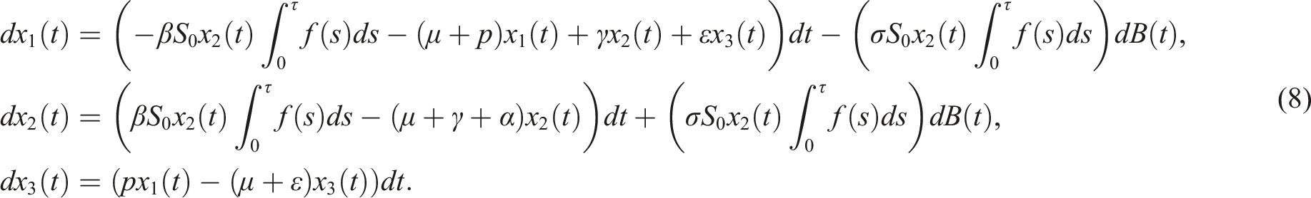
Assume the conditions Then, the trivial solution of (8) is asymptotically mean square stable.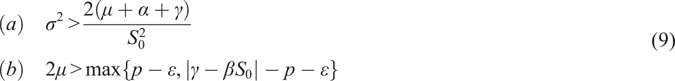
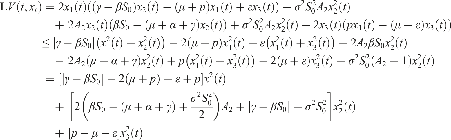
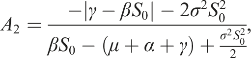
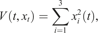
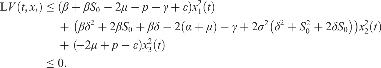
Choose the Lyapunov function Under conditions (9), choose A2 as follows Consequently

If conditions (9) hold, then the disease-free equilibrium of (3) is stochastically stable or equivalently, the trivial solution of (7) is stochastically stable.
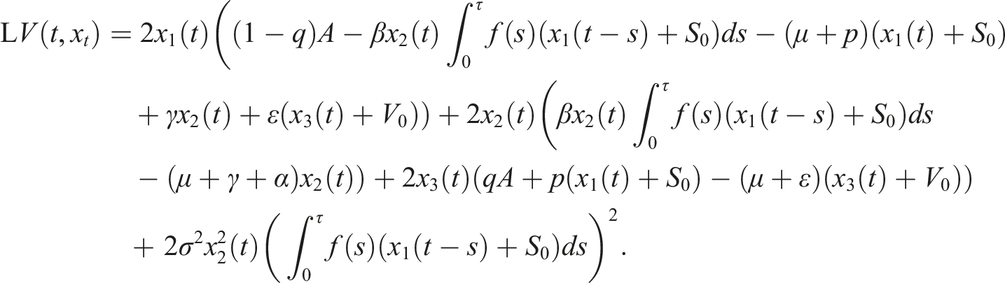
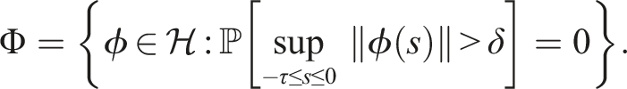
Under conditions (9), define a suitable δ > 0 such that Choose the Lyapunov functional in the form Then We have Then As x
t
∈ Φ, then This proves the stochastic stability of the disease-free equilibrium of (3).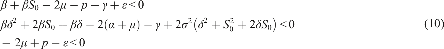
Stability in the mean
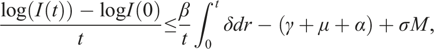
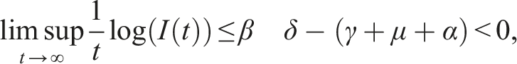
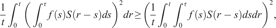
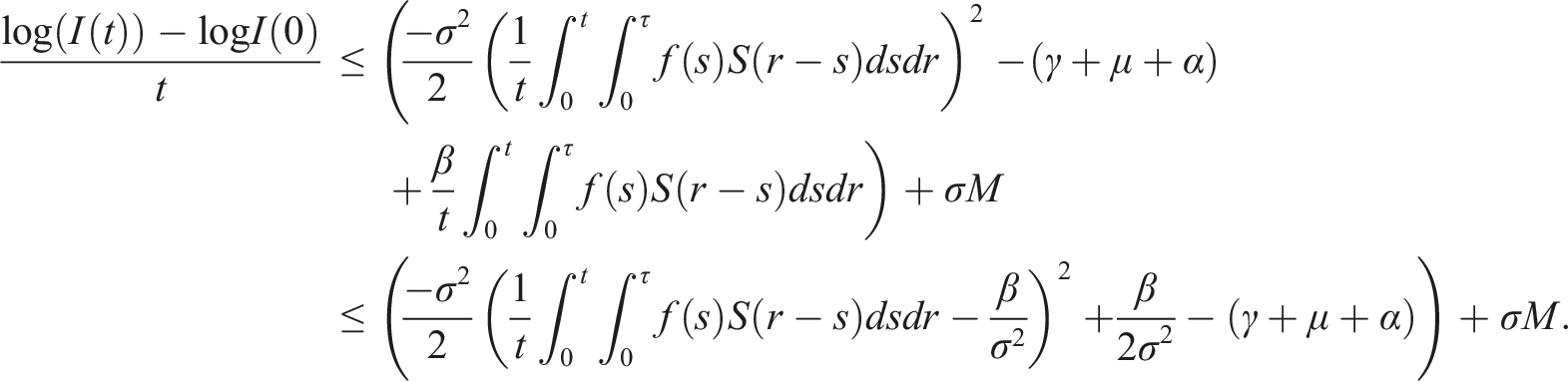
Here, we investigate the sufficient conditions for extinction through the stability of the disease-free equilibrium in the mean. Dedicated to these conditions, we introduce some numerical simulations that show the impact of the noise parameter on extinction. It is known that if R0 > 1, the deterministic system of SIS epidemic will persist. Regardless of the magnitude of R0 quantity, the disease dies out in the stochastic SIS model with distributed delays for small and large noises.
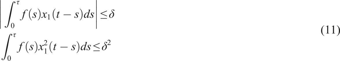
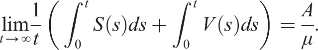
Assume that the solution (S(t), I(t), V(t)) and (ϕ1(θ), ϕ2(θ), ϕ3(θ)), θ ∈ [−τ, 0] are in Ω. If for arbitrary suitable δ > 0 Then Moreover
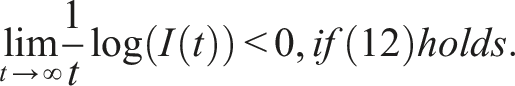
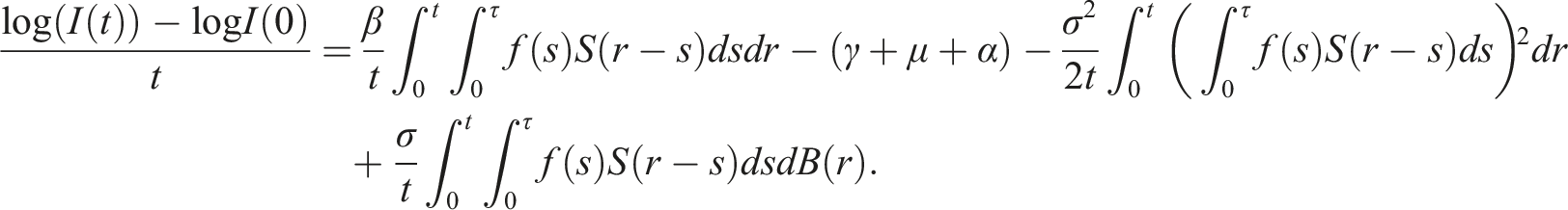
By introducing a suitable Lyapunov functional Integrating both sides and dividing by t imply Using Lemma (2.1) and (11), let And Accordingly Using the inequality Under condition (12), we get The integrating factor is As (13) holds with probability 1, we have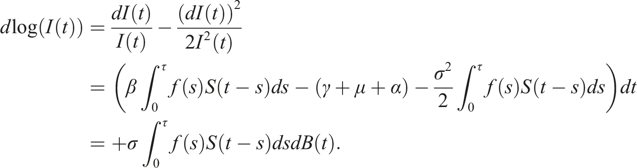


Numerical simulations and interpretation
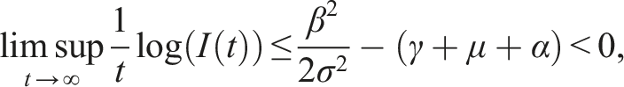
Mathematically, the disease dies out according to the stochastic stability conditions (9), and the intensity of the environmental stochastic perturbations of the transmission rate can help in the disease extinction. The disease-free equilibrium E0 is stable under small and large values of the noise parameter σ but we have much more restrictive conditions on the rate of losing immunity, it is bounded by
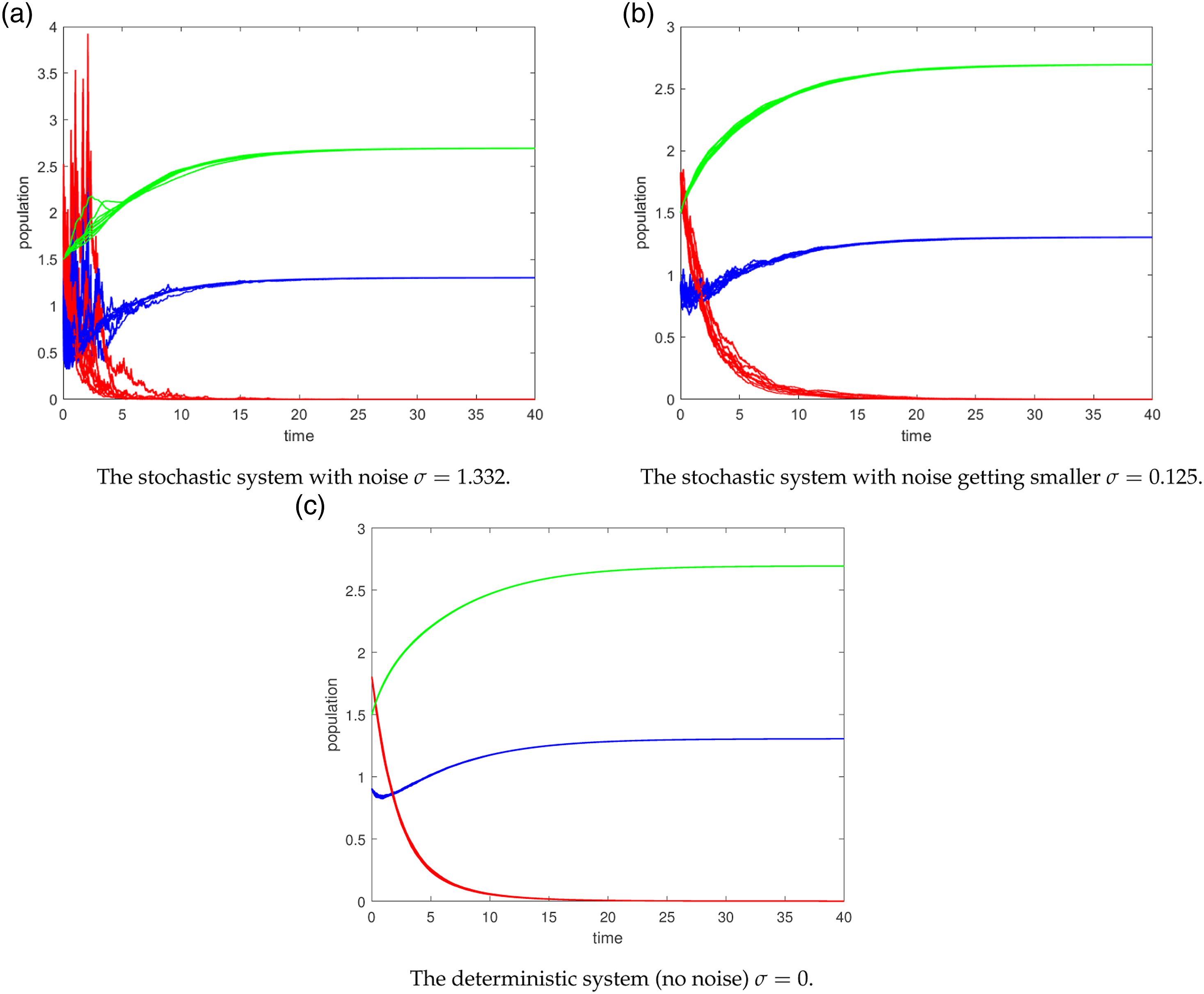
Numerical simulations have been conducted using 25 trajectories represented by different colors (blue, red, and green) to study the stability of the disease-free equilibrium. The results indicate that this equilibrium remains stable even when subjected to small levels of noise as well as under the influence of high levels of noise. In other words, the absence of the disease is maintained regardless of the presence of fluctuations, both in cases of low and high noise intensity.
Computer simulations are carried out for 25 (blue, red, green) trajectories of the path (S(t), I(t), V(t)) for (3) under condition (12). The disease-free equilibrium E0 = (1.305, 0, 2.694) is stable for β = 0.5 and R0 = 0.7678 < 1. (a) The stochastic system with noise σ = 1.332. (b) The stochastic system with noise getting smaller σ = 0.125. (c) The deterministic system (no noise) σ = 0.
We conducted two separate numerical simulations to investigate the behavior of a deterministic system and a stochastic system in the context of an epidemic. In the deterministic simulation Figure 3(a), the epidemic was characterized by a pandemic nature, with the disease persisting over time. The dynamics of the deterministic system go to the endemic equilibrium. However, when considering the stochastic system under the same parameter settings, a different outcome emerged: the disease-free equilibrium became stable, and the disease eventually died out, see Figure 3(b). The number of infected individuals goes to zero, consequently, E0 is stable regardless of the magnitude of R0. 25 (blue, red, green) trajectories of the path (S(t), I(t), V(t)) for (3) under condition (12). The dynamics deterministic system converges to the endemic equilibrium E* = (1.3, 0.083, 2.588) but the stochastic system dynamics converges to E0 = (1.305, 0, 2.694) for β = 0.7 and R0 = 1.0749 > 1. (a) The deterministic system (no noise) σ = 0. (b) The stochastic system with noise σ = 0.995.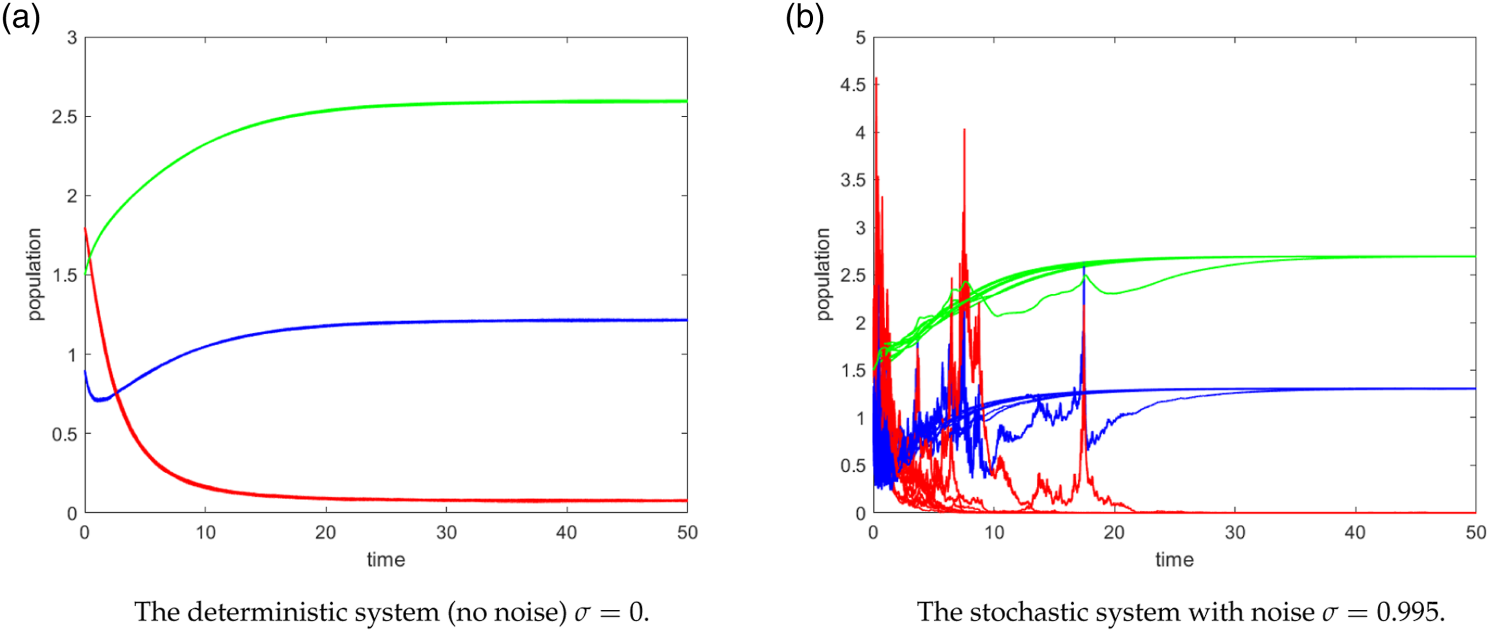
This intriguing result highlights the influence of noise in stabilizing an unstable deterministic system. Despite the initial tendency of the epidemic to persist in the absence of stochastic fluctuations, the introduction of noise had a stabilizing effect, leading to the eventual eradication of the disease. This phenomenon emphasizes the important role that random fluctuations can play in altering the dynamics of a system and potentially mitigating (possible extinction) the spread of infectious diseases.
While stochastic models with distributed delay have their advantages in capturing temporal dynamics, they also come with significant limitations that should be considered when using them in epidemiological research. First, the mathematical equations become more intricate, and numerical simulations may be required to solve them. Second, these models require detailed data on the progression of the disease, including information on the time taken for transitions between different stages.
A potential way for future research in epidemic modeling could involve incorporating a stochastic perturbation of fractional type, which offers a more general framework. By incorporating such a framework, it is expected that the dynamics of epidemics can be accurately described, accounting for the inherent randomness and long-range dependencies that exist in real-world epidemic processes.
Footnotes
Author contributions
The study presented here was carried out in collaboration between both authors I.M.E and M.A.S contributed to the selection and interpretation of the model. The theoretical analysis, numerical simulation of the model, and drafting of the manuscript were carried out by I.M.E. Critical revision of the manuscript was contributed to by H.M.E and I.M.E.
Declaration of conflicting interests
The author(s) declared no potential conflicts of interest with respect to the research, authorship, and/or publication of this article.
Funding
The author(s) disclosed receipt of the following financial support for the research, authorship, and/or publication of this article: This work was supported by the Open access funding is provided by The Science, Technology & Innovation Funding Authority (STDF) in cooperation with The Egyptian Knowledge Bank (EKB).
Data availability statement
Code availability
The codes used and/or analyzed during the current study are available from the corresponding author on reasonable request.