Sage Journals: Discover world-class research

Abstract

This paper investigates the sensitivity of structural system response to the sensor location by investigating consequences of small changes in the location to the structural system response. The paper discusses how maximum observability (based on mode shape and the participation of that mode in the input provided) drives optimal location. The structural responses were investigated in terms of the g-rms response for various low-frequency inputs (pure sinusoids and real-life inputs such as an earthquake and trains). Results were then analyzed in the context of Modal Contributions Factors (MCF) and changes to the Force-to-response Transfer Functions (TRFs). A modal-matching process is first presented using a Matlab^TM-based Finite Element Method (FEM) model of a cantilever beam and instrumentation to determine the location of a small mass based on three different criteria. Subsequently, the structural response is investigated using experiments and the FEM model. The accelerometer of small mass (at 1/3 height) was moved up or down to obtain changes in the structural response (TRF) to various realistic low-frequency inputs. Modal Contribution Factor (MCF) and derivative (slope) of the associated mode-shapes were correlated to the observed changes in TRFs. Results show how optimal sensor locations for detecting change in structural response can be based on the MCFs and the associated mode-shapes.

Keywords

structural dynamics modal contribution sensor location finite element testing

Sandia National Laboratories is a multimission laboratory managed and operated by National Technology & Engineering Solutions of Sandia, LLC, a wholly owned subsidiary of Honeywell International Inc., for the U.S. Department of Energy’s National Nuclear Security Administration under contract DE-NA0003525.

This paper describes objective technical results and analysis. Any subjective views or opinions that might be expressed in the paper do not necessarily represent the views of the U.S. Department of Energy or the United States Government.

Introduction

Experiments play a major role in research on structural dynamics and Structural Health Monitoring (SHM) based on modal parameters. While detecting the exact location of a mass may be less important, the location of a sensor to detect small changes in system dynamics is an important consideration for dynamics testing and SHM. A change in the Force-Response Transfer Function (TRF) in the frequency domain is a common parameter used in system identification. Deviations between the intended experiment and the experiment that is conducted can result in large errors, which may completely change the conclusions of a test if not properly addressed.¹ This situation forces the researcher to understand the sensitivity of the dynamic response of the system to these parameters and the uncertainty associated with factors that influence the test.^2–4 Such parameters, which are the subject of this paper, include input loads, boundary conditions, and sensor placement.

The presence of sensors on a System Under Test (SUT) can cause the system’s response to change. When these changes are too severe, researchers must find ways to adjust.^5–8 One method of doing this adjustment is by mitigating the effect of the sensor on the real system.^9–13 Researchers also include the mass of the sensor within a model to match their presence in an experiment. Once the model adequately matches the experiment, the sensor masses may be removed from the model to better simulate the behavior of the SUT in the field when no sensors are present. The decoupling procedures can be prone to severe error propagation.¹⁴ Another method of performing a Finite Element Model Update (FEMU) involves moving the mass of the sensors by updating the Mass Matrix.¹⁵ When sensor mass is significantly relative to the nodal mass of the FEM, focusing specifically on sensor location will yield results similar to reevaluating the entire mass matrix.

Full-field techniques for systems identification have been in vogue for many decades but have gained momentum due to the advancement of computer-vision hardware and data storage needs.¹⁶ Portability of devices is also increasing its application,¹⁷ considering the difficulty associated with access and site instrumentation of bridge structures. These techniques provide the added benefit of being completely non-invasive.

Recently, use of information theory to detect changes in structures is gaining prominence, due to the availability of data and advancements in computational power.^18,19 Papadimitriou¹⁸ has used information entropy (function of uncertainties in system parameters) as a measure of performance for systems identification.

The techniques proposed in this paper can help reconcile the differences between the initial state and subsequent changes to the system by identifying optimum sensor placement to detect changes in the system response to various realistic inputs.

The paper first presents the estimation of the location of an additional mass given the response data from a physical experiment. This estimate is achieved by creating a Finite Element Model (FEM) of a cantilever beam using the same geometric and material properties as the experimental beam. The modes are then altered with the added mass at various locations along its length until the model natural frequencies best match those of the test (Modal-matching method).

Subsequently, this paper investigates the changes to structural response of a cantilever beam by application of insights based on modal parameters as a function of sensor location. This analysis is demonstrated by finding the modal contributions of each mode at a range of frequencies and combining that information with the magnitudes of the input signal frequencies to indicate the extent to which each mode is relevant for a given input signal. The authors examine the variation in each mode for a change in sensor location to explain the changes observed in the experiment. These methods potentially enable optimal location of sensors in a physical experiment and provide a deeper understanding of how the changes in mass at a particular location affect the dynamic response of the system. Additionally, these techniques can be used to evaluate small changes in location of sensors in a test setup for detecting changes in structural dynamics. This approach is relevant for control of inputs in Multiple-Input Multiple-Output (MIMO) tests.

Experiment

Sensors and equipment

The test article consisted of a 34.5” high ×1.5” square (outside) × 1/8” thick (87.63 × 3.81 × 0.3175 cm) steel cantilever beam with a piezoelectric accelerometer magnetically attached at the tip. A second identical accelerometer (0.095 lb, 43 g) was moved between experiments and placed at three different locations.

This 43 g mass (approximately 5% relative to the 820 g mass of the beam) was selected so that small changes in its location impart a detectable change in the system dynamics. Lighter or non-contact sensors could be used but would not impart significant change to the system dynamics. It should be noted that for SHM of civil structures, the sensor mass is negligible to that of the structure. However, for mechanical components that is not necessarily the case and non-contact sensors are not feasible due to lack of line of vision to various regions of interest.

The three different locations of the sensor were 7/16^th of an inch (1.11 cm) above the one-third point, precisely at the one-third point, and 7/16^th of an inch (1.11 cm) below the one-third point. These were designated as the “Up,” “Centered,” and “Down” cases, respectively. The small change in location (1.11 cm) in the tests was based on being close to the diameter of the accelerometer 1.27 cm. Greater changes of sensor location would be easier to detect and were therefore beyond the scope of the paper. Based on this paper, consequences of greater change in location can also be evaluated by FEM analyses. The beam is excited by a stinger-based actuator, which connects to the beam at one-third the height with no variation in location. Figure 1 displays the three test setups for the three different accelerometer locations.

Figure 1.

Experiment setup with varying accelerometer location and DAQ.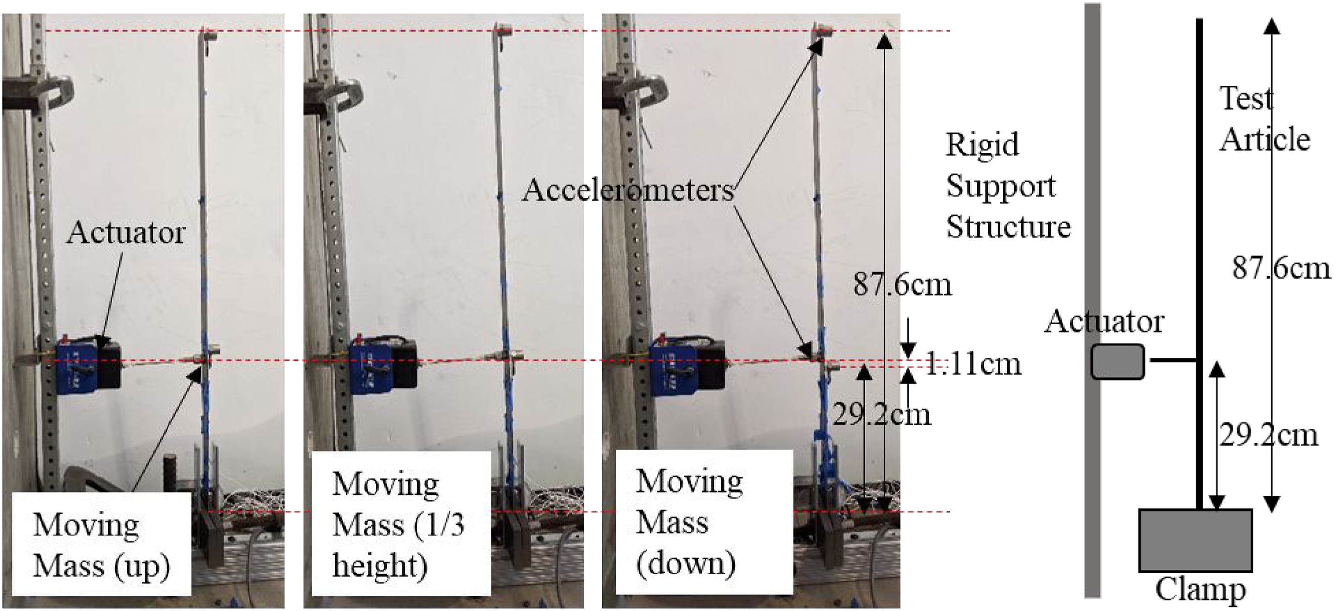

A piezoelectric accelerometer (PCB 353B03, ±500 g, resolution of 0.003 g 1 Hz−7 kHz) was placed at the tip of the beam to measure response to various inputs. The added mass referred to earlier was also an accelerometer (PCB 353B03), which could also be used to determine the response at that location. An electrodynamic shaker (K2007E01 Smartshaker^TM from Modal Shop Inc.) was used to excite the structure via nylon 10−32 stingers that connected to the beam with magnetic plates. This shaker has a double amplitude maximum stroke length of ½ of an inch (1.3 cm), a peak acceleration of 70 g when unloaded, or 3.3 g when loaded at maximum capacity with 8.9 N force. A load cell was placed between the stinger and the beam (PCB Model 208C02 with 445 N capacity, 0.0045 N resolution with a frequency range of 0.001 to 36,000 Hz). An 8-channel VibPilot^TM Data Acquisition system (DAQ) was used to receive data (24-bit analog-to-digital converters with up to 102.4-kHz anti-aliased sampling rate).

Tests with band-limited-white-noise (BLWN) input at 1/3 height

For each of the three physical setups with different location of the added mass, the structure was excited with a 30-second long Band-Limited (0−200 Hz) White Noise input. TRFs associated with each of the three configurations were obtained using equation (1)

\begin{array}{c} H (ω) = \frac{S_{X Y}}{\bar{S_{X X}}} \end{array}

(1)

where the H is a Transfer Function at frequency ω,

S_{X Y}

is the cross-spectral density of the input force and the output response, and

S_{X X}

is the auto-spectral density of the input force. Figure 2 presents these TRFs for the accelerometer at the tip location with respect to the force input at one-third height. Note that the modes 1 and 2 are <20 Hz, mode 3 is near 45 Hz, mode 4 is near 90 Hz, and mode 5 is near 150 Hz. There is an anti-resonance near 110 Hz between the fourth and fifth modes. These five modes seen in Figure 2 were also captured using the Finite Element Method (FEM) analysis. The anti-resonance near 110 Hz is due to the 1/3 location being at a node (acceleration due to different modes of opposing phase cancel each other at that location).

Figure 2.

TRFs (Tip Response to 1/3-Height Input) for the three different accelerometer locations.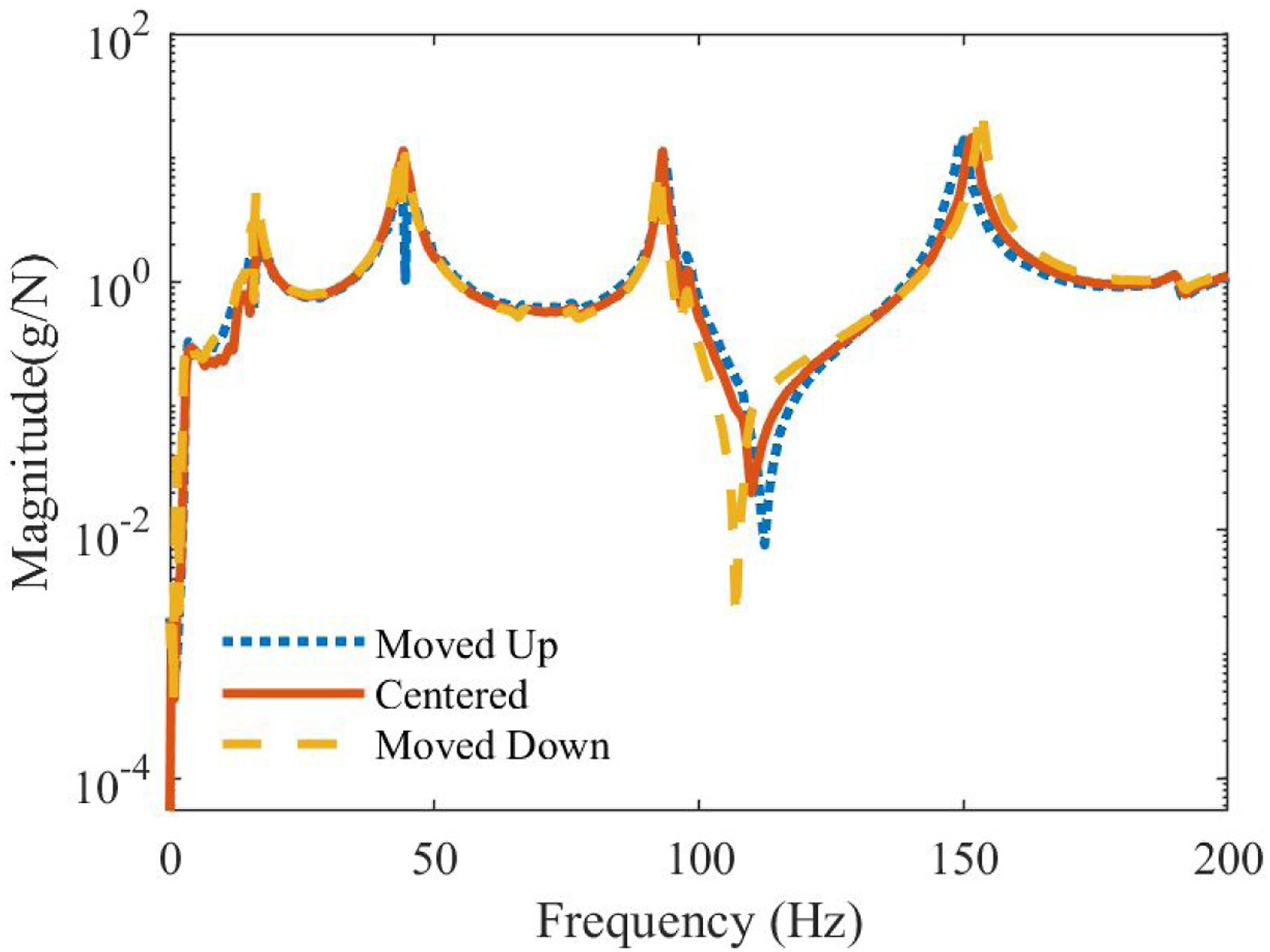

Finite element model

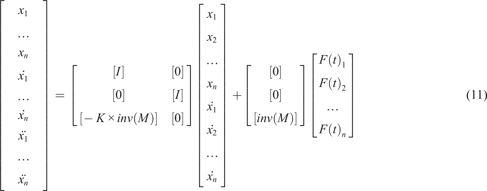
(Figure 3). Objective of the FEM model was to simulate the three test conditions (different accelerometer location with associated mass) and to perform analyses based on mode shapes and Modal Participation Factors. A Matlab^TM-based Finite Element Model (FEM) was created of the cantilever beam in the experiment using the same geometric and material properties. The model uses a damping coefficient obtained with Log-Decrement method from an initial free-vibration experiment on the same beam. The model was created and analyzed applying Euler–Bernoulli Beam theory with 552 elements representing the 34.5 × 1.5 × 0.125 inch (87.63 × 3.81 × 0.3175 cm) beam. Lump masses were located where sensors are centered to account for their effect on the beam dynamics. Each node is a cross section slice of the beam and is constrained to move only in the plane that bisects the broad face of the beam. As a result, the model only considers the bending modes within this plane. The resulting State-space model estimated the outputs for the beam per given inputs.

Figure 3.

Modal contributions at the tip from BLWN input at 1/3 height.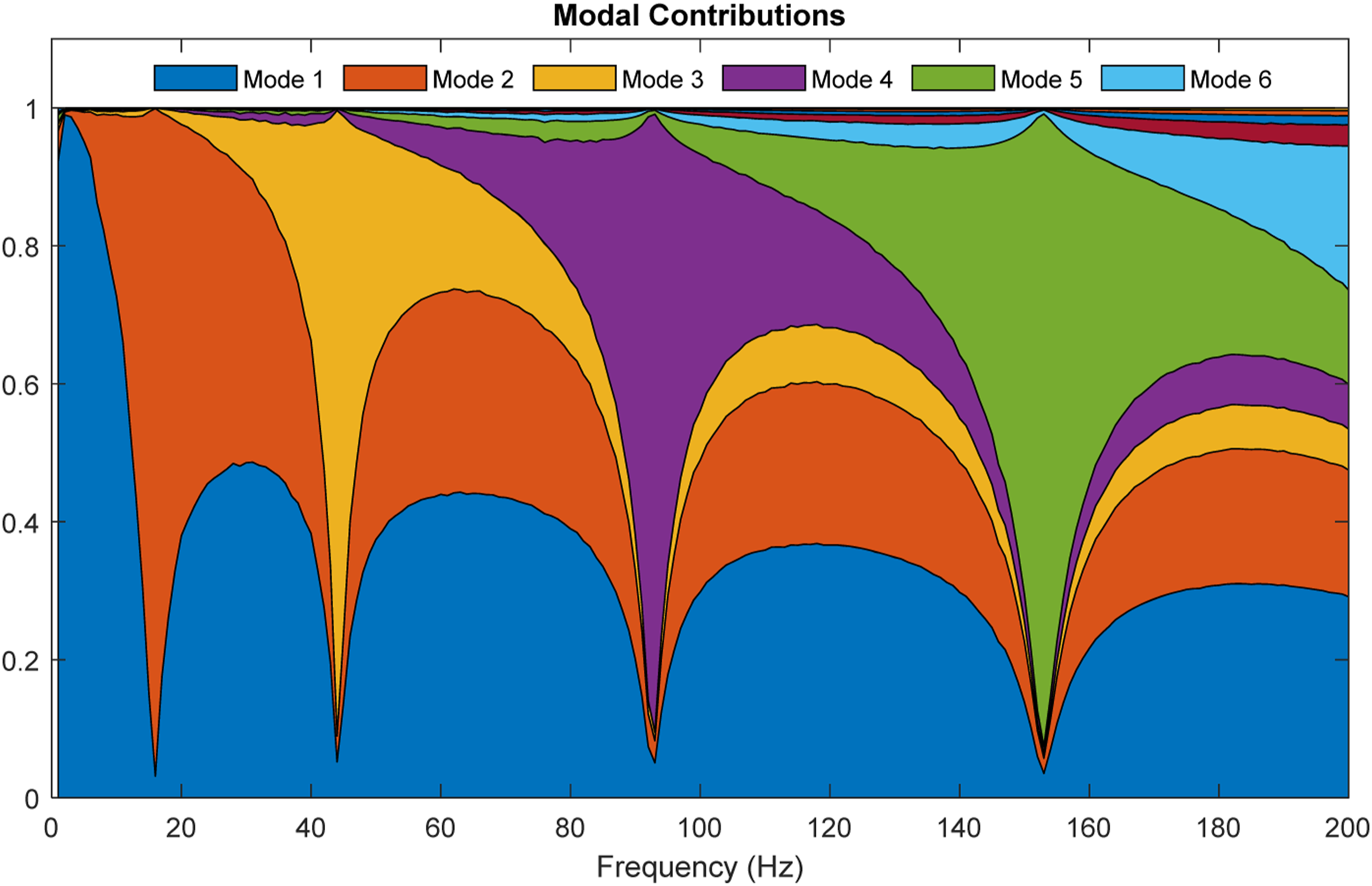

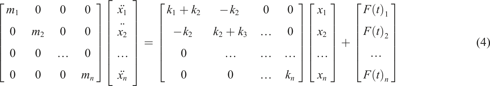
Based on Newton’s equations of motion

\begin{array}{c} \ddot{{m_{i} x}_{i} =} {F (t)}_{i} + x_{i} k_{i} + (x_{i} - x_{i + 1}) k_{i + 1} \end{array}

(2)

where

m_{i}

is the mass of node i,

\ddot{x_{i}}

is the acceleration at node i,

{F (t)}_{i}

is the external force applied at node i,

x_{i}

is the displacement at node i, and

k_{i}

is the stiffness of the element associated with node i. Defining the parameters as vectors and matrices, where n is the number of nodes

\begin{array}{c} p (t) = [\begin{array}{c} {F (t)}_{1} \\ {F (t)}_{2} \\ \dots \\ {F (t)}_{n} \end{array}], K = [\begin{array}{c} k_{1} + k_{2} & - k_{2} & 0 & 0 \\ - k_{2} & k_{2} + k_{3} & \dots & 0 \\ 0 & \dots & \dots & \dots \\ 0 & 0 & \dots & k_{n} \end{array}], M = [\begin{array}{c} m_{1} & 0 & 0 & 0 \\ 0 & m_{2} & 0 & 0 \\ 0 & 0 & \dots & 0 \\ 0 & 0 & 0 & m_{n} \end{array}] \end{array}

(3)

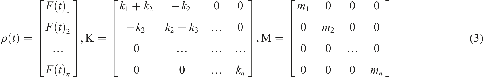
Therefore, rearranging into matrix form

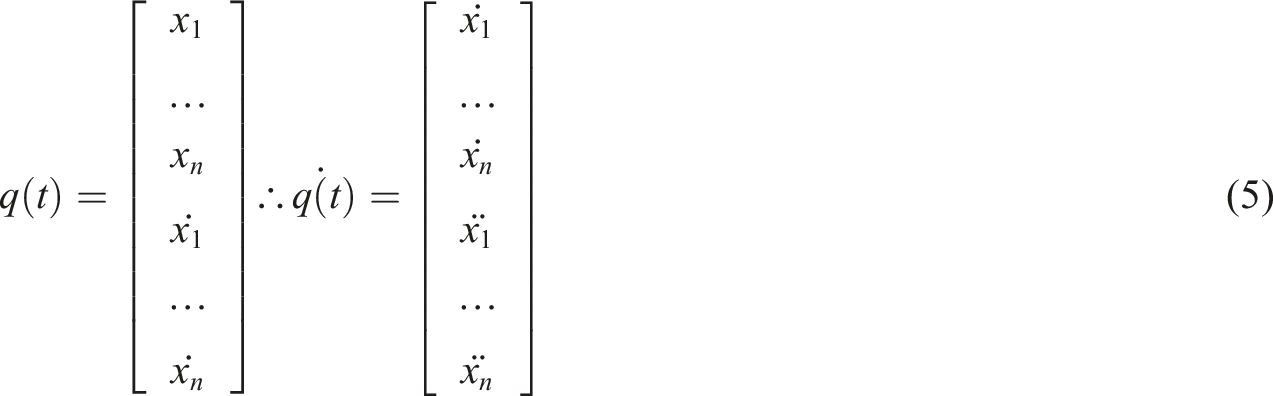
\begin{array}{c} [\begin{array}{c} m_{1} & 0 & 0 & 0 \\ 0 & m_{2} & 0 & 0 \\ 0 & 0 & \dots & 0 \\ 0 & 0 & 0 & m_{n} \end{array}] [\begin{array}{c} \ddot{x_{1}} \\ \ddot{\begin{array}{c} x_{2} \\ \dots \\ \ddot{x_{n}} \end{array}} \end{array}] = [\begin{array}{c} k_{1} + k_{2} & - k_{2} & 0 & 0 \\ - k_{2} & k_{2} + k_{3} & \dots & 0 \\ 0 & \dots & \dots & \dots \\ 0 & 0 & \dots & k_{n} \end{array}] [\begin{array}{c} x_{1} \\ x_{2} \\ \dots \\ x_{n} \end{array}] + [\begin{array}{c} {F (t)}_{1} \\ {F (t)}_{2} \\ \dots \\ {F (t)}_{n} \end{array}] \end{array}

(4)

Define state vectors $q (t)$ and $\dot{q (t)}$ as vectors of the beam response as given by the equations

\begin{array}{c} q (t) = [\begin{array}{c} x_{1} \\ \dots \\ \begin{array}{c} x_{n} \\ \dot{x_{1}} \\ \begin{array}{c} \dots \\ \dot{x_{n}} \end{array} \end{array} \end{array}] ∴ \dot{q (t)} = [\begin{array}{c} \dot{x_{1}} \\ \dots \\ \begin{array}{c} \dot{x_{n}} \\ \ddot{x_{1}} \\ \begin{array}{c} \dots \\ \ddot{x_{n}} \end{array} \end{array} \end{array}] \end{array}

(5)

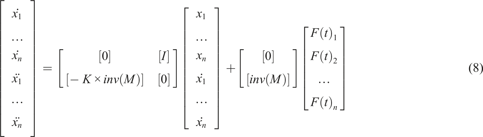
Define State Space Matrices State Matrix A and Input Matrix B such that

\begin{array}{c} [\dot{q (t)}] = [A] [q (t)] + [B] [p (t)] \end{array}

(6)

\begin{array}{c} A = [\begin{array}{c} [0] & [I] \\ [- K \times i n v (M)] & [0] \end{array}], B = [\begin{array}{c} [0] \\ [i n v (M)] \end{array}] \end{array}

(7)

where [0] is n × n matrix of zeros, and [I] is n × n identity matrix.

Combining into the State equation

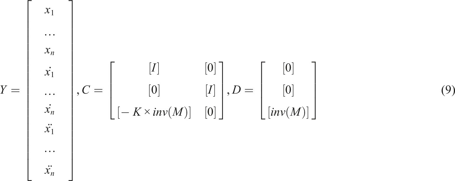
\begin{array}{c} [\begin{array}{c} \dot{x_{1}} \\ \dots \\ \begin{array}{c} \dot{x_{n}} \\ \ddot{x_{1}} \\ \begin{array}{c} \dots \\ \ddot{x_{n}} \end{array} \end{array} \end{array}] = [\begin{array}{c} [0] & [I] \\ [- K \times i n v (M)] & [0] \end{array}] [\begin{array}{c} x_{1} \\ \dots \\ \begin{array}{c} x_{n} \\ \dot{x_{1}} \\ \begin{array}{c} \dots \\ \dot{x_{n}} \end{array} \end{array} \end{array}] + [\begin{array}{c} [0] \\ [i n v (M)] \end{array}] [\begin{array}{c} {F (t)}_{1} \\ {F (t)}_{2} \\ \dots \\ {F (t)}_{n} \end{array}] \end{array}

(8)

The vector Y represents the total output as found by multiplying $q (t)$ by the output matrix C and $p (t)$ by the feedthrough matrix D. Since this example examines the outputs of all nodes, the output equation effectively just builds on the state space equation

\begin{array}{c} Y = [\begin{array}{c} x_{1} \\ \dots \\ \begin{array}{c} x_{n} \\ \dot{x_{1}} \\ \begin{array}{c} \dots \\ \begin{array}{c} \dot{x_{n}} \\ \begin{array}{c} \ddot{x_{1}} \\ \begin{array}{c} \dots \\ \ddot{x_{n}} \end{array} \end{array} \end{array} \end{array} \end{array} \end{array}], C = [\begin{array}{c} [I] & [0] \\ [0] & [I] \\ [- K \times i n v (M)] & [0] \end{array}], D = [\begin{array}{c} [0] \\ [0] \\ [i n v (M)] \end{array}] \end{array}

(9)

\begin{array}{c} [Y] = [C] [q (t)] + [D] [p (t)] \end{array}

(10)

Substituting equations (9) into (10)

\begin{array}{c} [\begin{array}{c} x_{1} \\ \dots \\ \begin{array}{c} x_{n} \\ \dot{x_{1}} \\ \begin{array}{c} \dots \\ \begin{array}{c} \dot{x_{n}} \\ \begin{array}{c} \ddot{x_{1}} \\ \begin{array}{c} \dots \\ \ddot{x_{n}} \end{array} \end{array} \end{array} \end{array} \end{array} \end{array}] = [\begin{array}{c} [I] & [0] \\ [0] & [I] \\ [- K \times i n v (M)] & [0] \end{array}] [\begin{array}{c} x_{1} \\ x_{2} \\ \dots \\ x_{n} \\ \dot{x_{1}} \\ \dot{x_{2}} \\ \dots \\ \dot{x_{n}} \end{array}] + [\begin{array}{c} [0] \\ [0] \\ [i n v (M)] \end{array}] [\begin{array}{c} {F (t)}_{1} \\ {F (t)}_{2} \\ \dots \\ {F (t)}_{n} \end{array}] \end{array}

(11)

Results of tests and analyses

Modal-matching to determine location of the moving mass

The FEM model was verified using just the eigenvalues to compare the first five modes to those measured from the experiment. The process of model verification was based on “modal matching” and consisted of the following steps:

• The mass of the accelerometer at 1/3 height was placed at various nodes along the length close to the 1/3 height location where it was actually placed during the experiment.

• The 1^st five predicted modes were compared to those from the FEM eigenvalues.

• The sum of the absolute differences of the five modes was calculated. The minimum sum is expected to correspond to the actual location of the mass (at 1/3 point).

This paper investigates three metrics [equations (12)−(14)] to score the model location setups and defines the sensor location setup with the lowest value of the metric to be the location estimated by the FEM model. These metrics are the Total Deviation of the mode frequencies [equation (12)], the Maximum Deviation [equation (13)], and the Total Relative Deviation [equation (14)]. The one-third location, at 11.5 inches (29.2 cm) from the base of the beam, was set as the datum for these comparisons

\begin{array}{c} T o t a l D e v i a t i o n (T D) = \sum_{i = 1}^{5} | {Exp}_{i} - {Mod}_{i} | \end{array}

(12)

where

{Exp}_{i}

is the frequency of mode i as found in the experiment and

{Mod}_{i}

is the frequency of mode i as taken from the eigenvalues of the FEM for a given sensor location setup

\begin{array}{c} M a x i m u m D e v i a t i o n (M D) = \max (| Exp - Mod |) \end{array}

(13)

\begin{array}{c} T o t a l R e l a t i v e D e v i a t i o n (T R D) = \sum_{i = 1}^{5} | \frac{({Exp}_{i} - {Mod}_{i})}{{Exp}_{i}} | \end{array}

(14)

Finally, the Total Difference (last row in Table 1) was calculated by adding (for the three locations) the difference between the location predicted by the three methods and the nominal (actual) location.

Table 1.

Estimated sensor location using modal matching.

Location of Mass predicted by modal-matching
Mass location	Nominal	Total deviation	Maximum deviation	Total relative deviation
Moved up	7/16”(1.11 cm)	11/16” (1.75 cm)	9/16” (1.43 cm)	7/16” (1.11 cm)
Centered	0	0	−1/8” (0.32 cm)	0
Moved down	−7/16” (−1.11 cm)	−11/16” (−1.75 cm)	−7/8” (−2.22 cm)	−19/16” (3.0 cm)
Total difference		1/2” (1.3 cm)	11/16” (1.75 cm)	3/4” (1.9 cm)

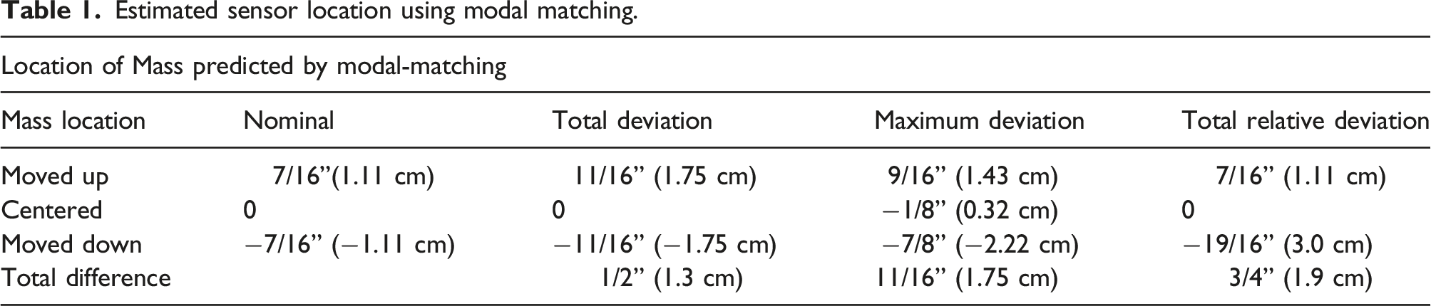
Based on results shown in Table 1, the Total Deviation metric scored the lowest and best of the three metrics; the best match (minimum sum of differences) corresponded to the accelerometer locations 11/16” (1.75 cm) above and below the 1/3 height, while the actual accelerometer locations were 7/16” (1.11 cm) above and below the 1/3 height. This agreement demonstrated that the modal-matching could accurately capture the added mass as well as its location to ¼” (0.64 cm) accuracy.

Modal-contribution factor to optimize sensor location

Determination of MCFs

The modal contribution method offers more insight to sensor placement towards accurate measurement of TRFs. Using the MCF and Modal-matching techniques complementarily, one can use modal contributions to inform experiment setup while using model-matching to identify the location of the added mass. Using MCF can help establish which modes are most relevant for a given frequency, how that information will affect the results, and how this technique can inform a researcher in performing an experiment. Researchers traditionally use Modal Contributions for Modal Superposition, whereby the force vibration response for a given input is estimated as a combination of different mode shapes at different magnitudes. Modal Contributions indicate the extent to which each mode is relevant for an input at a given frequency. Using Modal Superposition, a force vibration response is summed by equation (15)

\begin{array}{c} y = \sum η_{i} Ф_{i} \end{array}

(15)

where y is the response estimate,

η_{i}

is the modal contribution factor for mode i, and

Ф_{i}

is the mode shape of mode i. Putting the equation into matrix form and rearranging, one can solve for

η

for each frequency, given the force vibration response

\begin{array}{c} {η}_{j} = {[Ф]}^{- 1} {y}_{j} \end{array}

(16)

where

{η}_{j}

is the vector of Modal Contribution Factors (MCF) corresponding to a vibration at frequency j, and

{y}_{j}

is the relative force vibration envelope for a vibration at frequency j. In practice, the study only used the first ten modes due to the negligibility of higher modes within the frequency domain examined.

The force vibration response from a Band Limited White Noise (BLWN) input at the one-third point in the FEM model was used to estimate the TRFs of each node along the cantilever beam. The magnitude of these TRFs at a given frequency then represent the relative response experienced at that frequency, resulting in the force vibration response used to find the Modal Contributions. Figure shows the percentile Modal Contributions at each frequency at 1 Hz increments from 1 to 200 Hz. Note that at 30 Hz both modes 1 and 2 are significant, at 45 Hz mode 3 is dominant, at 90 Hz mode 4 is dominant and at 150 Hz mode 5 is dominant. These MCFs will be used next to investigate sensitivity of sensor location with respect to the relevance of each mode.

Tests and analyses with sinusoidal inputs

Tests were conducted to investigate the effects of moving the mass at 1/3 height (up or down 7/16″, 1.11 cm from the center) on the time domain using the following steps:

• A sinusoidal time-history of the same amplitude was input (at 1/3 height) at a specific frequency at a time (not sine-sweep) (30–150 Hz range at 15 Hz intervals).

• Response at the tip and 1/3 height were measured and compared to that determined from multiplying the input with the TRF determined from the BLWN experiment reported earlier for the mass located at the 1/3 height (using 10 second steady state windows from 30 second tests).

• Differences in the root-mean-square (rms) acceleration (g) of the two signals were compared (relative to the measured g-rms) to determine the changes reported in Figures 4 and 5. Figures 4 and 5 also show the TRFs for response at the tip and 1/3 height from the FEM model.

Figure 4.

Changes to the structural response at the tip for various frequencies.

Figure 5.

Changes to the structural response at 1/3 height for various frequencies.

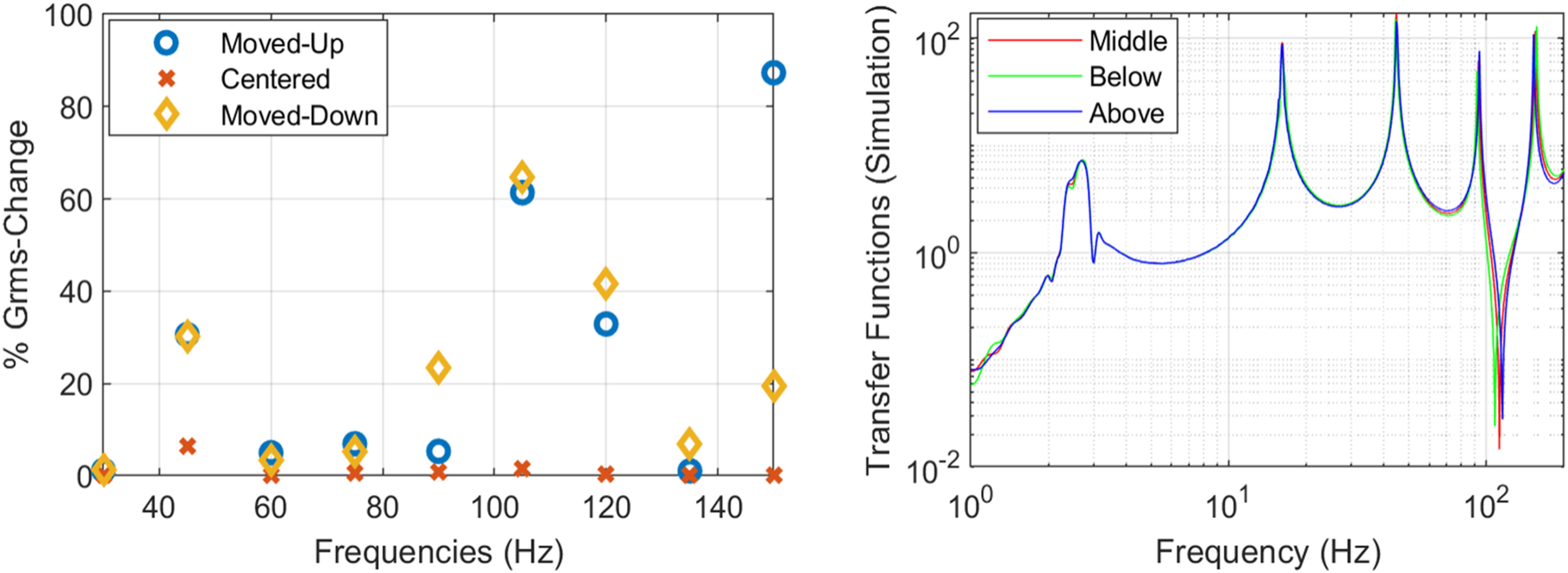
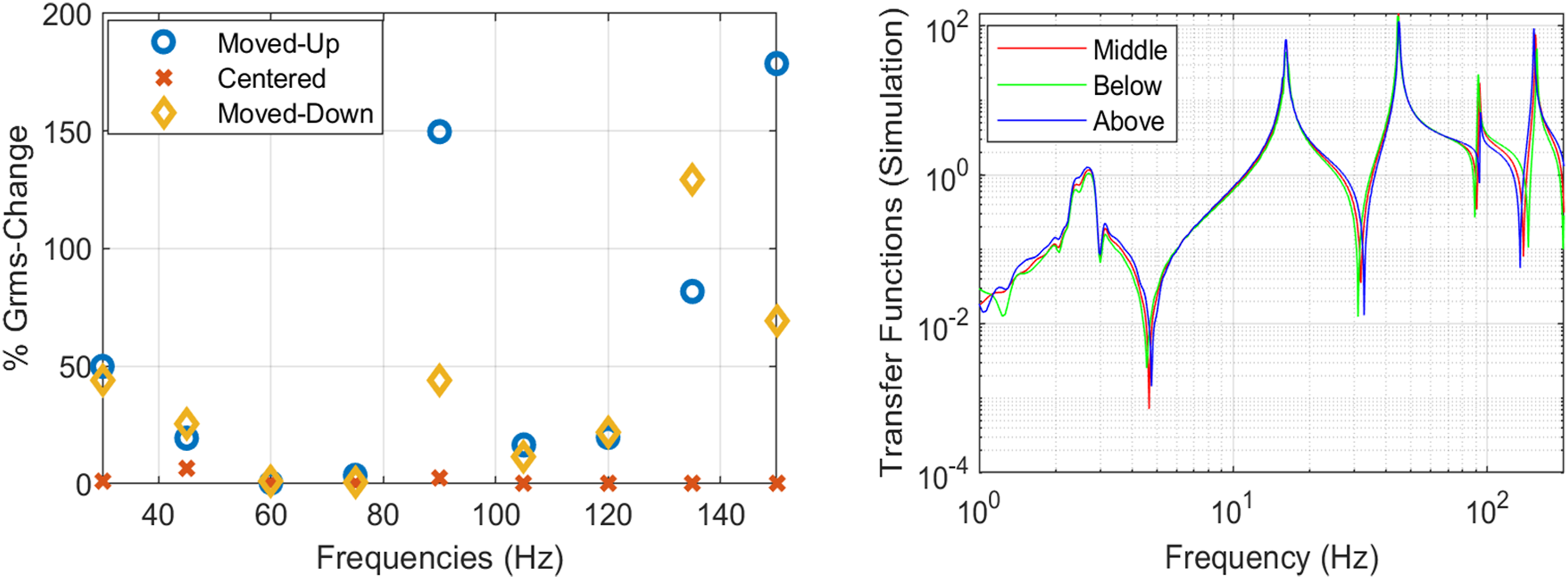
In Figures 4 and 5 the small changes reported for the “Centered” -case represent the combination of any test-to-test variation and any errors in processing of the signals. Note that the largest %changes in g-rms are at 45 Hz, 90 Hz, and 150 Hz (resonances) and 105−120 Hz (anti-resonances). The TRF for the 1/3 height location also has antiresonances near 30 Hz and 135 Hz, explaining the higher error in Figure 5 at those frequencies. The focus of this analysis is near the resonances where the vibration energy is concentrated.

Explaining changes in structural response from the sinusoidal input tests

In order to explain the changes to the structural response g-rms due to the moving mass shown in Figures 4 and 5, the FEM model was used to determine the TRFs at the tip. Results are shown in Figures 6 and 7, which capture the first five modes at 2.7, 16, 45, 94, and 154 Hz (comparable to that shown in Figure 2 from the experiment). Differences in the TRFs at the relevant peaks (45, 90, and 150 Hz) are shown by zooming in at those frequencies. TRF varies much more at the anti-resonances (≈110 Hz). Mode shapes corresponding to these first five modes from the FEM model are shown in Figure 7 along with the location of the tip and the 1/3 height (black lines). The thicker lines correspond to the change in the mode-shapes due to moving the mass up versus down, scaled (x10) to make them more visible on the same plot. The following observations can be made:

Figure 6.

Transfer function at tip accelerometer from FEM model.

Figure 7.

First five mode shapes and scaled g-rms change for modes 3–5.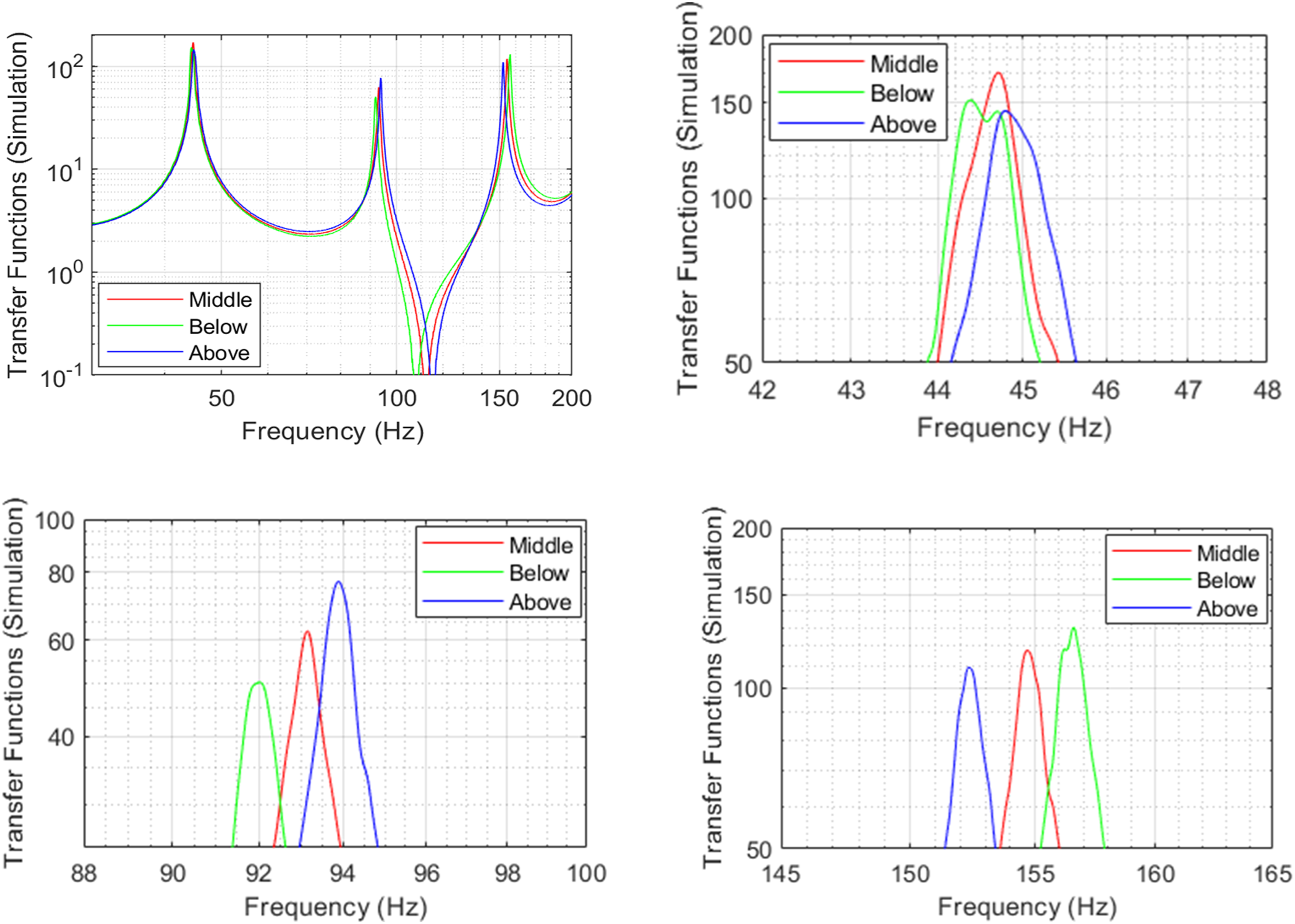

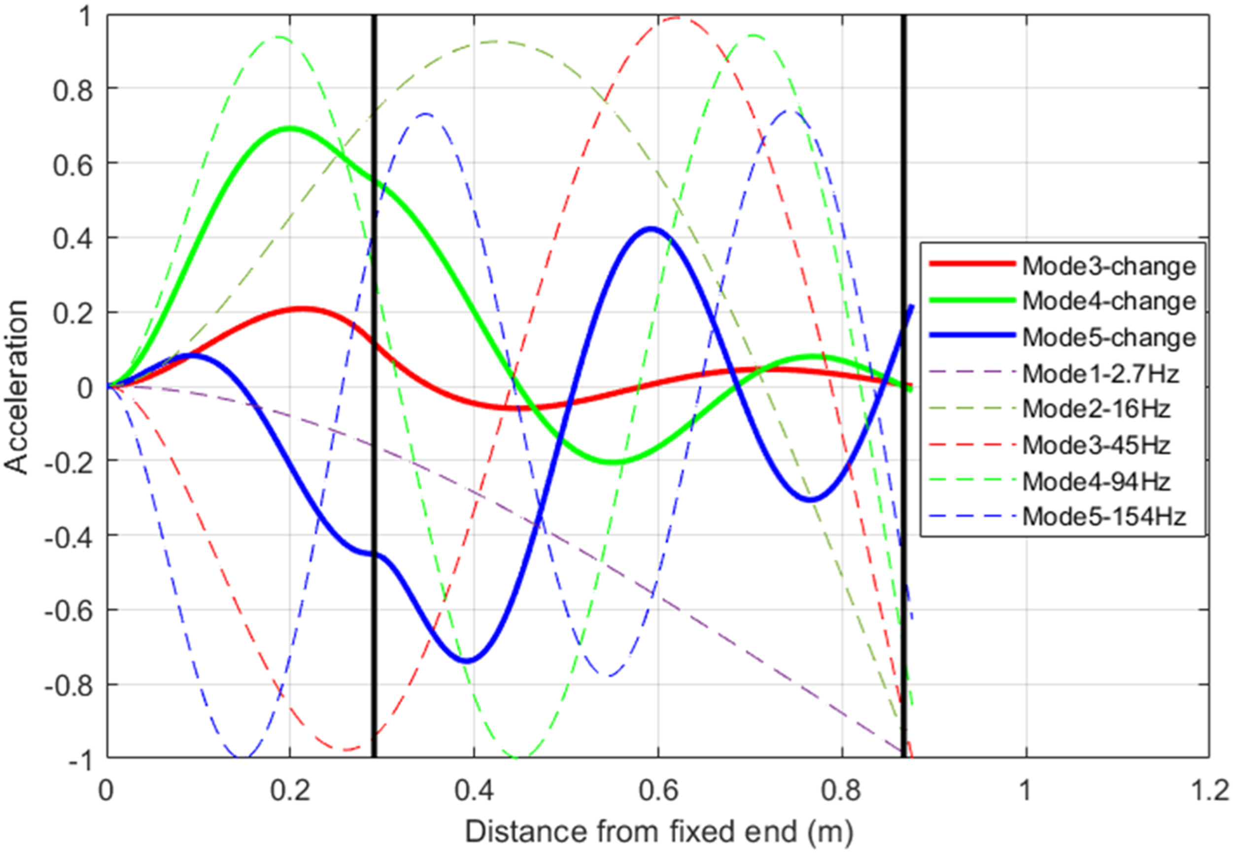
Figure 6 shows that near modes 3 and 4 (45 and 90 Hz) moving the mass higher (above) causes less motion (see mode shape) hence the frequency increases, while moving the mass lower (below) the frequency decreases. The opposite is seen for mode 5; moving the mass higher (above) causes more motion and the frequency decreases. Therefore, the direction of shift due to the added mass can be determined from the mode-shape. Figure 7 also shows that at the tip, the change in mode 5 (154 HZ) is more prominent than that for modes 3 and 4, which corresponds to the greater %change at 155 Hz than at 90 or 45 Hz seen in Figure 4 (left). At the 1/3 location, modes 5 and 4 show greater change than mode3, consistent with the higher %changes at 90 and 155 Hz than at 45 Hz in Figure 5 (left). Therefore, the sensor location most susceptible to change for particular frequencies can be determined from modal analyses.

Tests and analyses with realistic inputs (earthquake and trains)

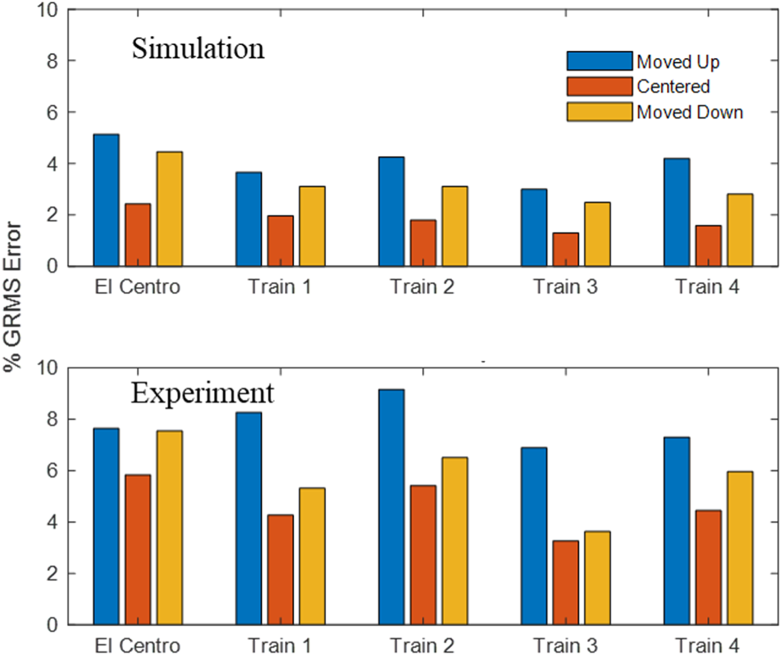
The tests and simulations discussed in the previous section for the nine harmonic signals were repeated with five different broad-band signals to demonstrate the application of the same principles based on (MCFs). The five input signals consisted of the El Centro Earthquake, as well as four signals based off measured train crossing events on the Bluford bridge, a timber bridge near Edgewood, Illinois. A 10-second window (24,576 points) of the primary excitation event from each signal was used as indicated in Figure 8.

Figure 8.

Broadband input time signals (earthquake and trains).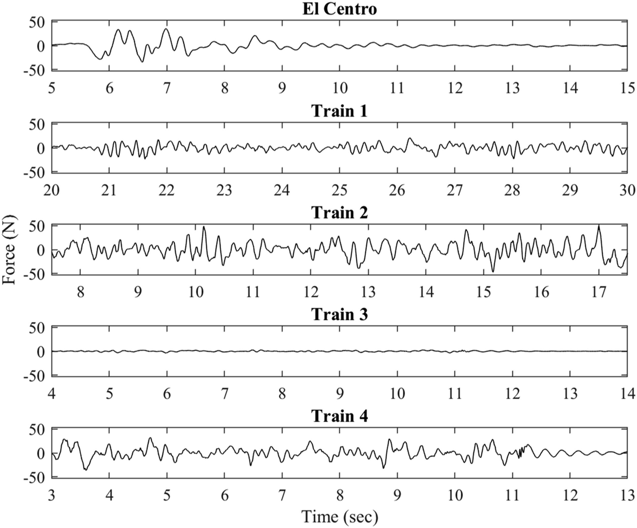

Frequency content of the five inputs is shown in Figure 9. All the signals were near the 1^st mode, but Train 2 had significant mode 2 content. Except for Train 3, each signal is also roughly equal in amplitude, peaking around an absolute value of 10 lbf (44.5 N). Once again, the g-rms-errors were computed for the three different locations of the mass at 1/3 height. Figure 10 displays the results of performing this analysis with both a simulation based on the FEM and a physical experiment case.

Figure 9.

Frequency content of the five inputs (1lbf = 4.45 N).

Figure 10.

Broadband input results: FEM simulation and experiment.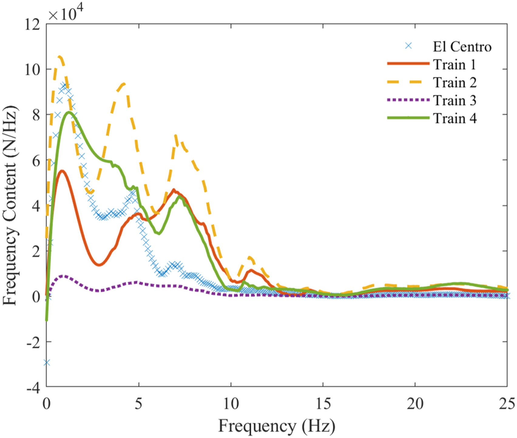

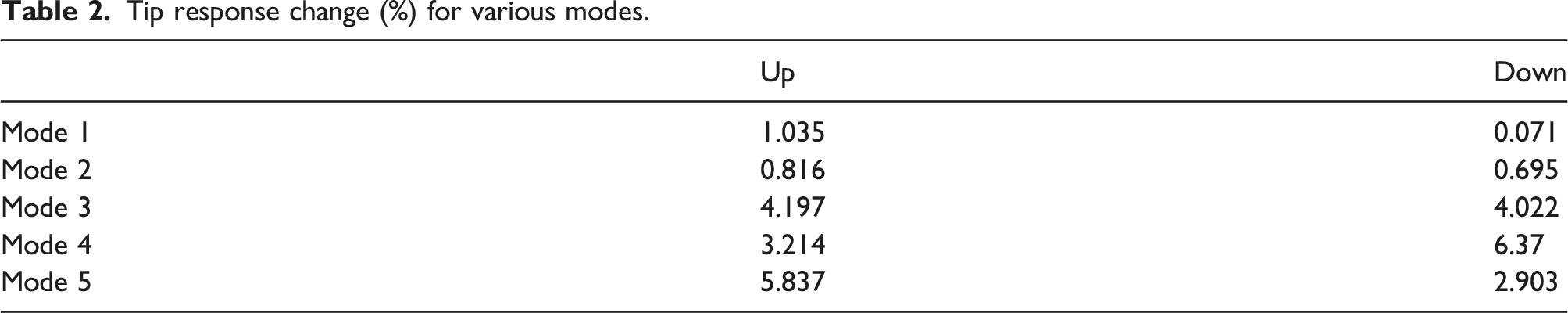
It can be observed from Figure 10 that the overall magnitude of the error with this metric is notably lower than in the harmonic cases. This observation is due to the fact that at a given frequency, the change in sensor location will have a given effect, either increasing or decreasing the amplitude of the time history. However, in a broadband signal, some frequencies witness an increase in magnitude, while others decrease. This variability results in a more stable overall magnitude for the time history. As expected, the Center case error (simulation) is consistently the lowest because only numerical error is contributing. The physical experiment has much higher error than the simulation due to test-to-test variation. Train 3 has magnitude of error similar to the other broadband tests despite having a much lower input magnitude. This result shows that even with very small force inputs, the sensor location has a notable effect on the structural response. Table 2 displays the extent to which the tip magnitudes for each of the natural frequencies change with a 7/16^th inch (1.11 cm) change in mass location. Table 3 provides the Modal Contribution Factors for the five inputs.

Table 2.

Tip response change (%) for various modes.

	Up	Down
Mode 1	1.035	0.071
Mode 2	0.816	0.695
Mode 3	4.197	4.022
Mode 4	3.214	6.37
Mode 5	5.837	2.903

Table 3.

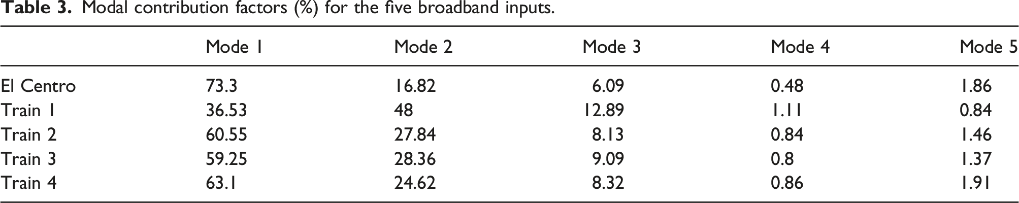
Modal contribution factors (%) for the five broadband inputs.

	Mode 1	Mode 2	Mode 3	Mode 4	Mode 5
El Centro	73.3	16.82	6.09	0.48	1.86
Train 1	36.53	48	12.89	1.11	0.84
Train 2	60.55	27.84	8.13	0.84	1.46
Train 3	59.25	28.36	9.09	0.8	1.37
Train 4	63.1	24.62	8.32	0.86	1.91

In both the simulation and the physical experiment, the Moved Up case error is more significant than the Moved Down case. Looking to modal properties, modal contributions, and the input signal frequency content, the increased errors in the Moved Up case can be qualitatively predicted. This estimate is due to the fact that mode 1 varies more for an upward movement than a downward movement, and that most of the energy in these broadband inputs is concentrated in mode 1.

Table 2 can also help explain the errors shown in Figure 4 for the sinusoidal inputs:

• At 45 Hz mode 3 dominates and the mass moved down or up have similar errors.

• At 90 Hz mode 4 dominates and mass moved down has higher error than mass moved up.

• At 150 Hz mode 5 dominates and mass moved up has higher error than mass moved down.

Therefore, the combination of Table 2 and the MPFs for the five inputs (Table 3) helps explain the sensor location effects observed in Figure 10.

Conclusions

Experiments were conducted for various pure sinusoids as well as real-life inputs (earthquake and trains) to the structure. Results of the experiments were analyzed with a Matlab^TM-based FEM model developed for this research.

A modal-matching process using the FEM model was able to determine the location of a small mass added to the structure, evaluating three different criteria for determining the location.

Changes in structural response (in terms of % g-rms and Transfer Function) were used for direction of a small (7/16”, 1.11 cm) change in the location of the mass. This analysis was done for various types of inputs using the (MCF) and slopes of the associated mode shapes to explain g-rms errors due to changes in the structural response.

It was shown that the sensor location most susceptible to change for particular frequencies can be determined from modal analyses. Therefore, the effect of sensor location in the context of modal contributions can help determine optimum locations for detection of changes in response for different types of input loads. The resulting insight can also be used for system identification or (SHM). While this paper involves a cantilever beam, the concept can be easily extended to more complex structures using FEM analyses to identify modal quantities.

Additionally, these techniques can be used to evaluate small changes in sensor location in test setups for detecting changes in structural dynamics or for Multiple-Input Multiple-Output (MIMO) testing where inaccuracies accumulate into erroneous inputs.

Footnotes

Declaration of conflicting interests

The author(s) declared no potential conflicts of interest with respect to the research, authorship, and/or publication of this article.

Funding

The author(s) disclosed receipt of the following financial support for the research, authorship, and/or publication of this article: The financial support of this research is provided by Sandia National Laboratories Grant 1985700, under Project Manager Dr John Pott, Manager, Environments Engineering, to whom the authors are grateful.

ORCID iD

A Maji

References

Vinot

Cogan

Cipolla

. A robust model-based test planning procedure. J Sound Vib 2005; 288(3): 571–585. DOI: 10.1016/j.jsv.2005.07.007.

Friswell

Coote

Terrell

, et al. “Experimental data for uncertainty quantification”. In: Proceedings of the 23rd international modal analysis conference, Orlando, FL, 2005. Society of Experimental Mechanics (SEM).

Tondreau

Deraemaeker

. Numerical and experimental analysis of uncertainty on modal parameters estimated with the stochastic subspace method. J Sound Vib 2014; 333: 4376–4401. DOI: 10.1016/j.jsv.2014.04.039.

Michaelides

Fassois

. “Stochastic identification of structural dynamics from multiple experiments – experimental variability analysis”. In: Proceedings of the ISMA conference, Belgium, Europe, 2008.

Ashory

, Assessment of the mass-loading effects of accelerometers in modal testing. In: Proceedings of the 20th international modal analysis conference, Los Angeles, CA, 4–7 February 2002, pp. 1027–1031.

Koruk

. “Quantification and minimization of sensor effects on modal parameters of lightweight structures”. J. Vibroengineering 2014; 16(4): 1952–1963.

Dossing O Prediction of transducer mass-loading effects and identification of dynamic mass. In: Proceedings of the ninth international modal analysis conference (IMAC9), Florence, Italy, 15–18 April 1991.

McConnell

. Vibration testing, theory and practice. New York, NY: Wiley, 1995.

Decker

Witfeld