
Abstract
In this study, the famous fractional generalized coupled cubic nonlinear Schrödinger–KdV equations arising in many domains of physics and engineering such as depicting the propagation of long waves in dispersive media and the dynamics of short dispersive waves for narrow-bandwidth packet have been investigated. We propose two significant methods named the modified (Gʹ/G, 1/G)-expansion method and the Gʹ/(bGʹ + G + a)-expansion method. After utilizing these two efficient techniques, many types of explicit soliton pulse solutions including the well-known bell-shape bright soliton pulse, the kink and anti-kink dark solitons pulse, the mixed bright-dark soliton pulse, the W-shaped soliton pulse, the periodic waves pulse, and the blow-up soliton pattern solutions are obtained. If we select different values of the frequency, coefficients and orders, the dynamic properties and physical structures of these solutions are discussed, these important results can help us to further understand the inner characteristic of the model.
Keywords
Introduction
In the last several decades, many topics in nonlinear dispersive partial differential equations especially for the fractional-order models have been characterized, such as soliton propagation for explaining the oceanic phenomena that correlate to nonlinear shallow or deep-water wave propagation,1,2 the interactions of capillary-gravity water waves between short and long dispersive waves arising in fluid mechanics, 3 the vector rogue waves in coupled vector nonlinear Schrödinger equations, 4 the suppression of chaotic oscillations, 5 the market dynamics characteristic, 6 the optical fiber communication, 7 etc.8–9 For better explaining the complex feature of these phenomena, searching for analytic explicit solutions including approximate solutions and exact solutions of these models plays an important and significant role. Up to now, many powerful methods for this subject such as the homotopy analysis method (HAM), 10 He’s homotopy perturbation method (HPM), 11 Adomian’s decomposition method (ADM), 12 variational iteration method (VIM), 13 Laplace transformation method, 14 double Laplace transform method, 15 Yang-Laplace transformation method, 16 and Shehu transformation method 17 can be used to find the approximate solutions. The Bäcklund transformation method, 18 Darboux transformation, 19 and Hirota bilinear method 20 can be used to find the N-soliton solutions. The improved F-expansion method, 21 projective Riccati equations method, 22 Jacobi elliptic function expansion method, 23 Gʹ/G-expansion method, 24 (d + Gʹ/G)-expansion method, 25 (Gʹ/G, 1/G)-expansion method, 26 sine Gordon method, 27 Lie symmetry method, 28 new Kudryashov’s method, 29 auxiliary equation method, 30 exponential rational function method, 31 etc.32–42 can be used to find doubly periodic solutions, solitary wave solutions, and trigonometric function solutions of these models. More research on the exact solutions, approximate solutions, and dynamic analysis of fractional systems can be found in Refs. [43-47].
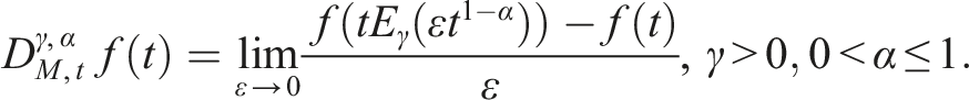
As we all know, calculus was founded by Newton and Leibniz at the second half of the 17th century, and fractional order calculus has gradually become one of the new special fields in natural sciences since 1695. 48 Till now, several types of definitions about the fractional derivative operator and integral operator are discussed and established by many researchers, the classical forms including Riemann–Liouville fractional derivatives, 49 Caputo fractional derivatives, 50 He’s fractional derivative, 51 Jumarie fractional derivative, 52 Atangana’s fractional derivative, 53 conformable fractional derivative, 54 Abu-Shady–Kaabar fractional derivative,55–57 and the M-fractiona derivative26,58,59 which will be utilized in this article.
In the present article, we consider the following M-fractional generalized coupled cubic nonlinear Schrödinger–KdV equations (MFCNLS-KdV) in the form Refs. [60–65].
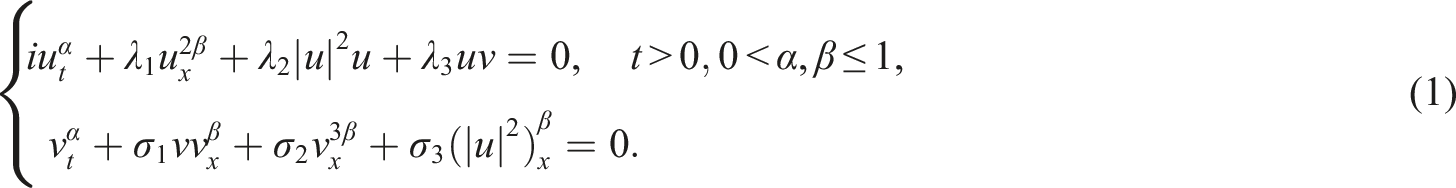
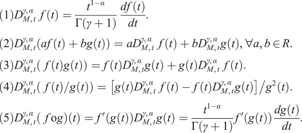
For a function Also, we have the following important properties26,58,59 In this article, we will propose two efficient and significant methods for finding some new types of exact solutions of equation (1) and many important results are obtained. The paper is organized as follows: In the Description of the two methods section, we introduce the modified (Gʹ/G, 1/G)-expansion method and the Gʹ/(bGʹ + G + a)-expansion method. While in the Exact solutions to the MFCNLS-KdV section, some new types of soliton pulse solutions of the MFCNLS-KdV are found and discussed by utilizing the proposed method. Finally, the conclusion is presented in the Conclusion section.
Description of the two methods
The modified (Gʹ/G, 1/G)-expansion method
The (Gʹ/G, 1/G)-expansion method has been proposed by many authors recently.68,69 We give some formal modification about this method in order to simplify the solving procedure for equation (1), a brief description of the technique is presented as follows:
Consider the following nonlinear M-fractional partial differential equation

Using a wave transformation70,71


Assume that equation (4) has the following solution


When

When

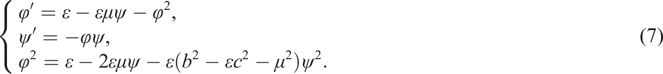
Substituting equations (7) and (5) into equation (4), and setting the coefficients of
Notice that the Refs. [68,69] were focused on collecting the coefficients of
The Gʹ/(bGʹ + G + a)-expansion method
With the similar procedure about the technique 2.1, we give the main steps about this method.
Assume that equation (2) has the following solution Equation (12) admits the following solutions.


When
When
Substituting equations (10) and (12) into equation (4), and setting the coefficients of In the following, we will use these two methods to solve the MFCNLS-KdV.
Exact solutions to the MFCNLS-KdV
Exact solutions
We can give the following function and traveling wave transformation


Substituting equations (13) and (14) into equation (1), separate the real part and the imaginary part, we obtain
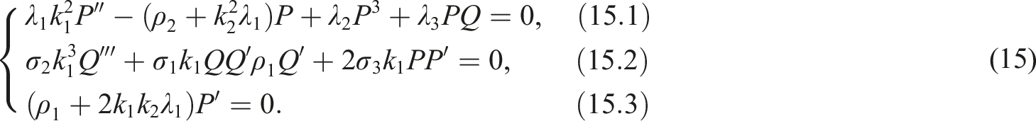
Substituting equation (15.3) into equation (15.2), then integrate once, we obtain
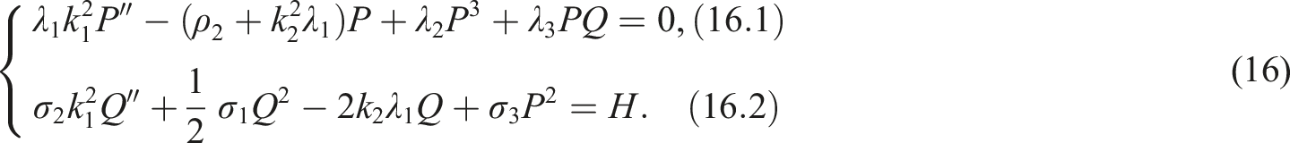
We assume that

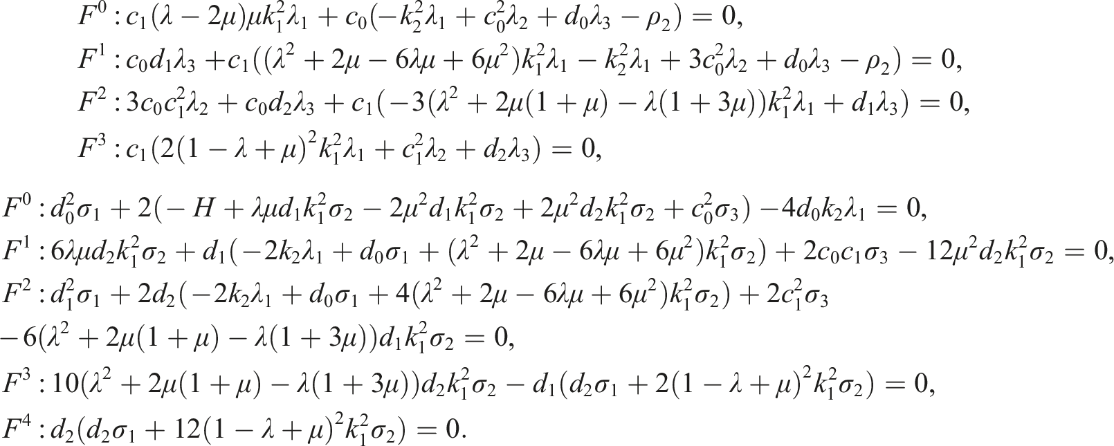
Substituting equations (17) and (7) into equation (16), and setting the coefficients of
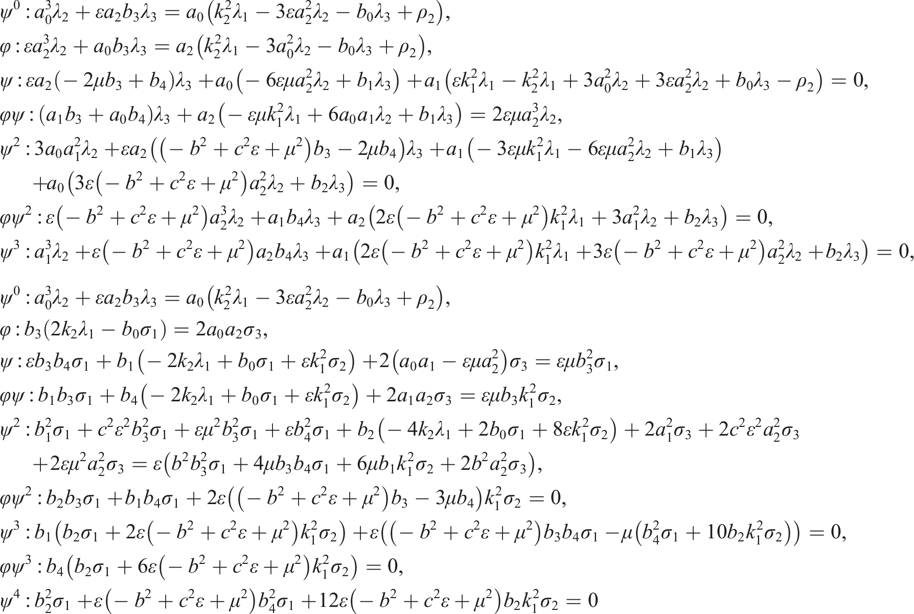
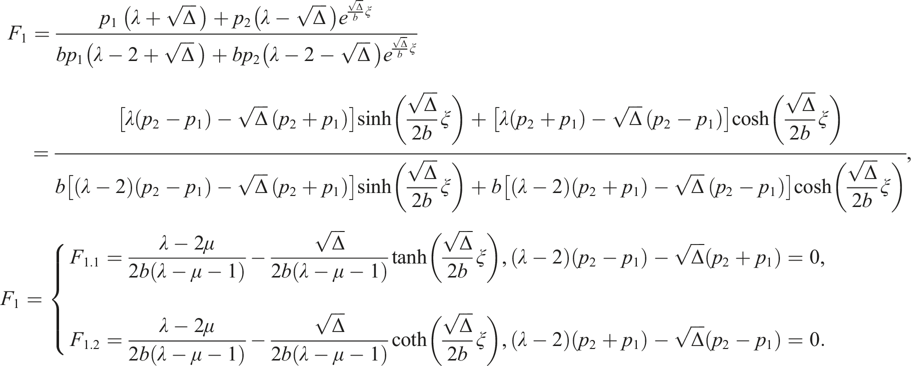
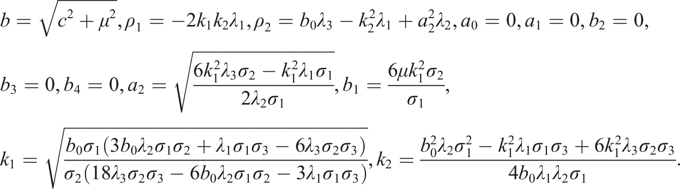
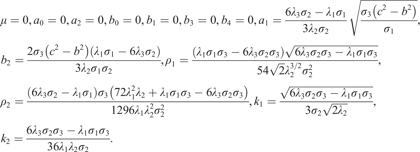
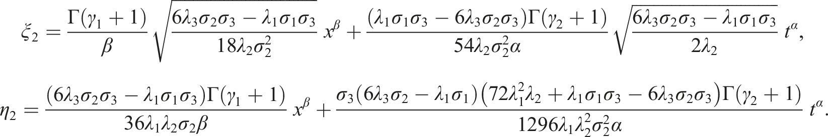
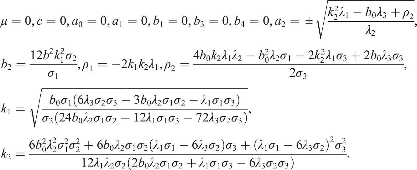
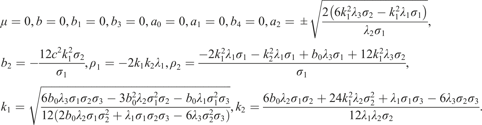
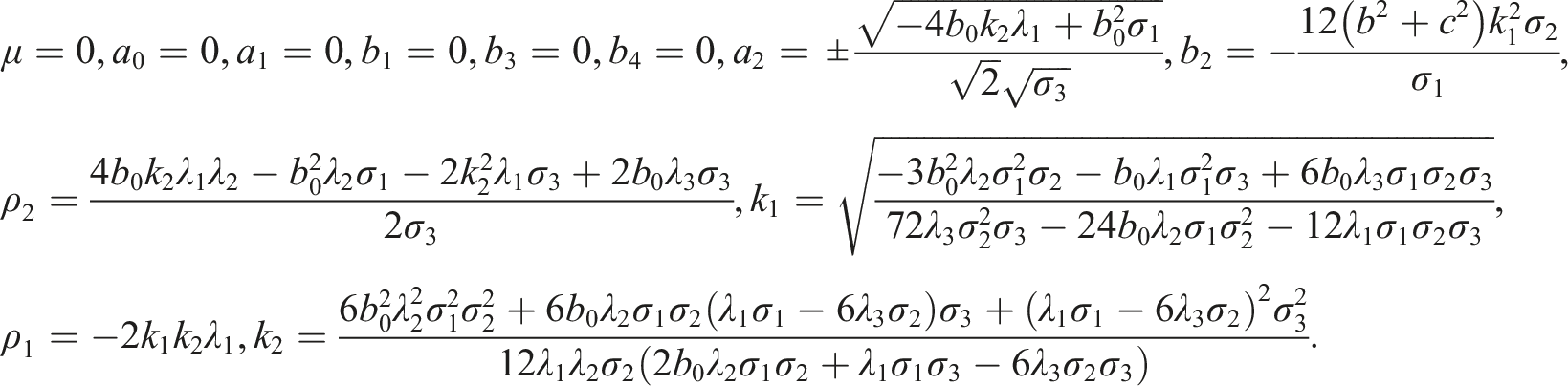
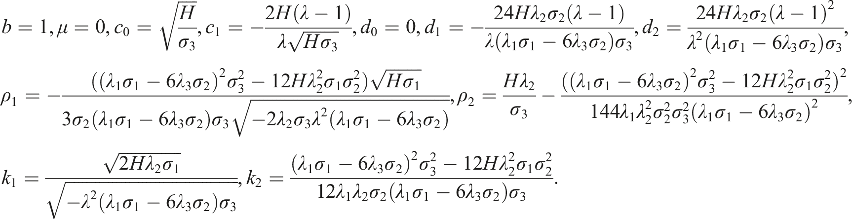
After solving the AEs along with equations (13) and (14), we could determine the following solutions
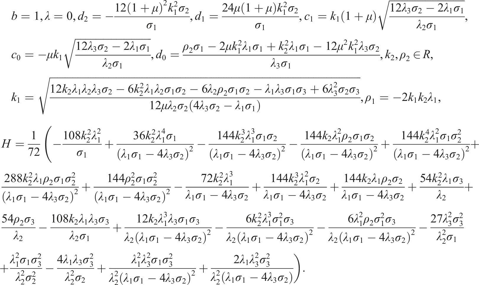
In this situation, we produce the following solutions of the above AEs
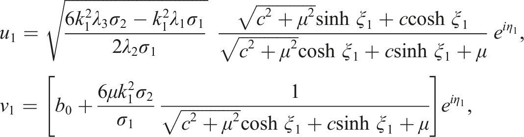
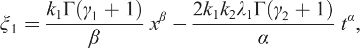
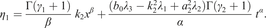
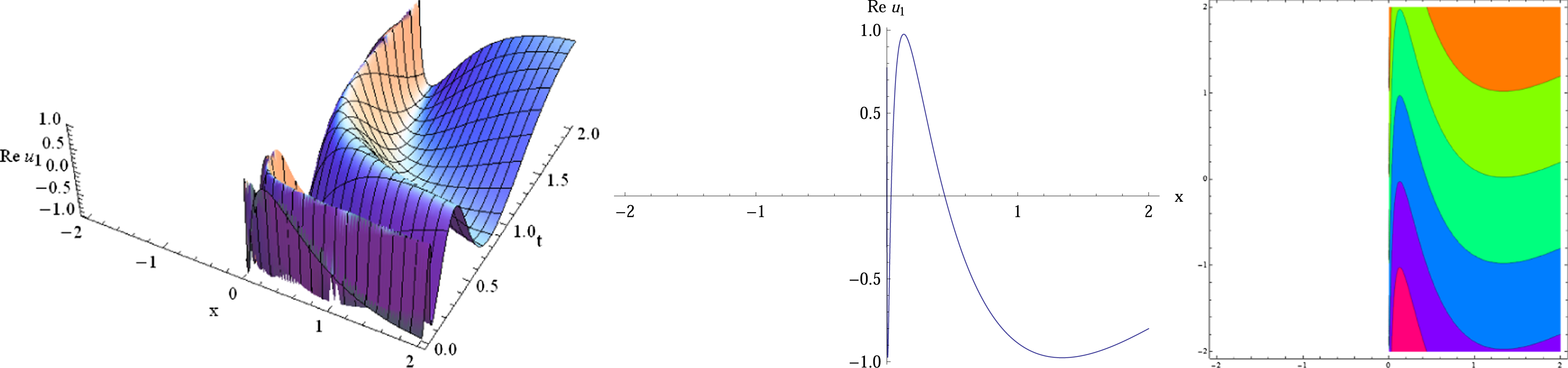
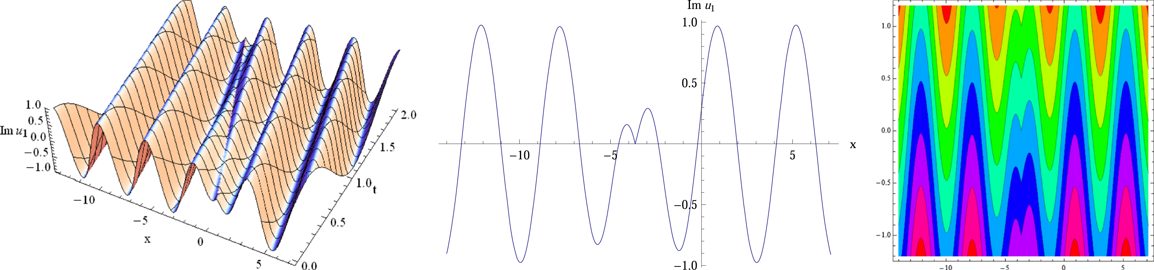
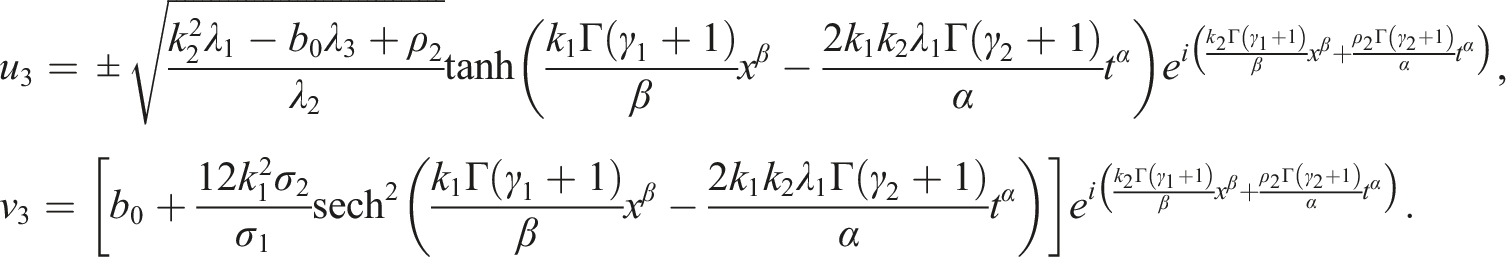
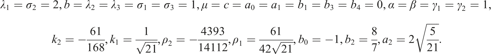
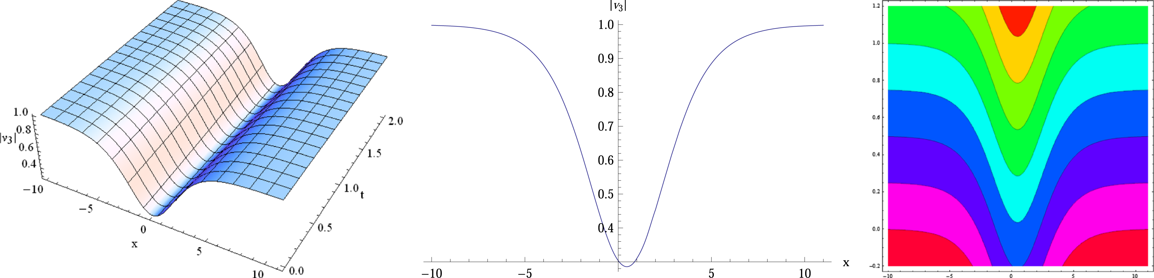
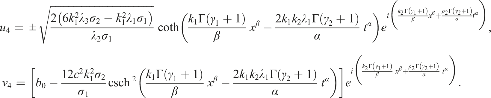
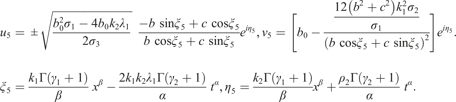
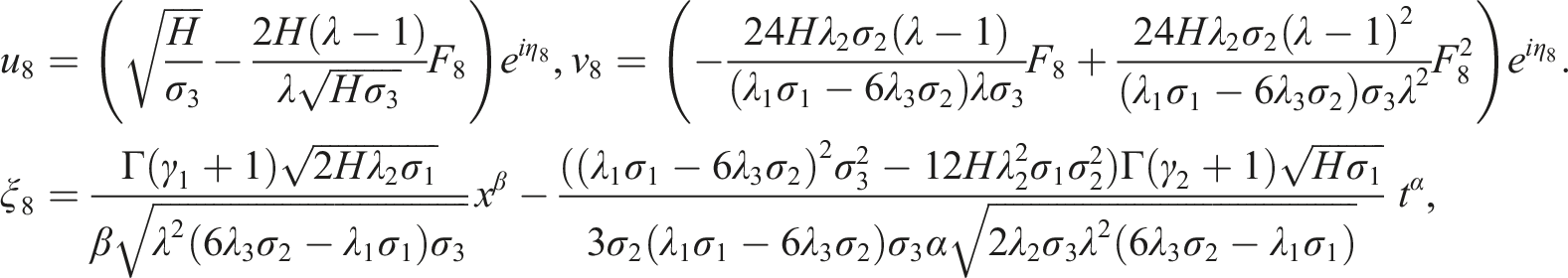
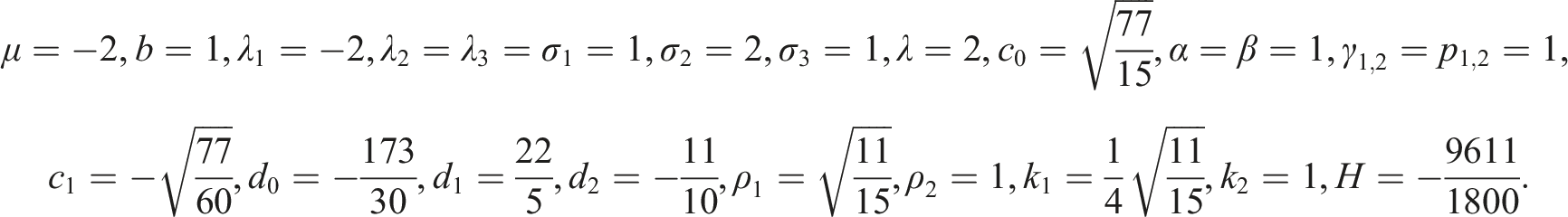
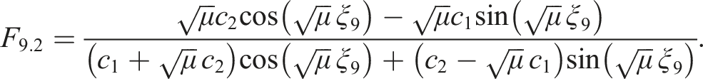
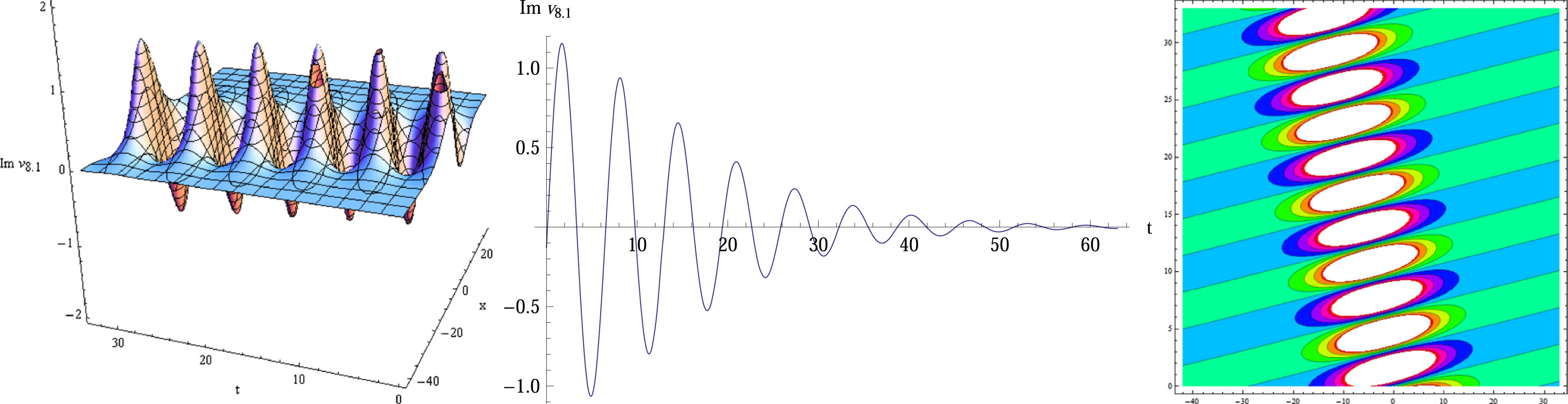
From equations (8), (13), (14), and (17), we can deduce the traveling wave solution of equation (1) as follows Selecting the following parameters in
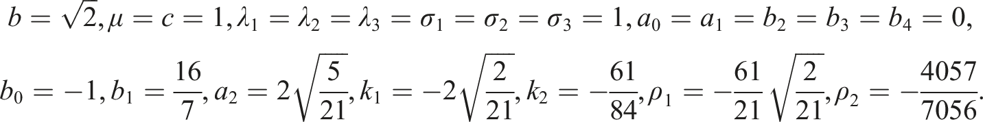
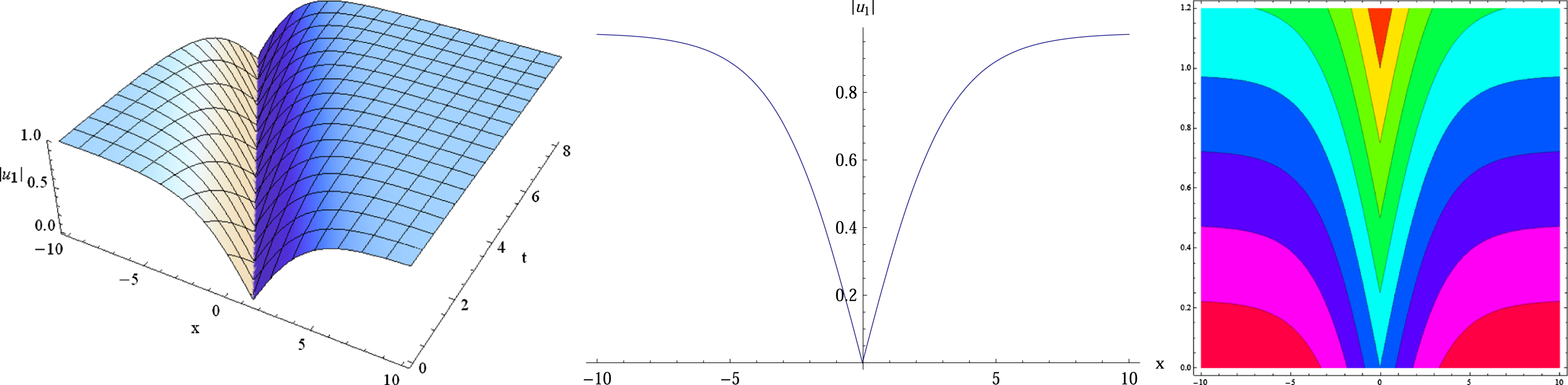
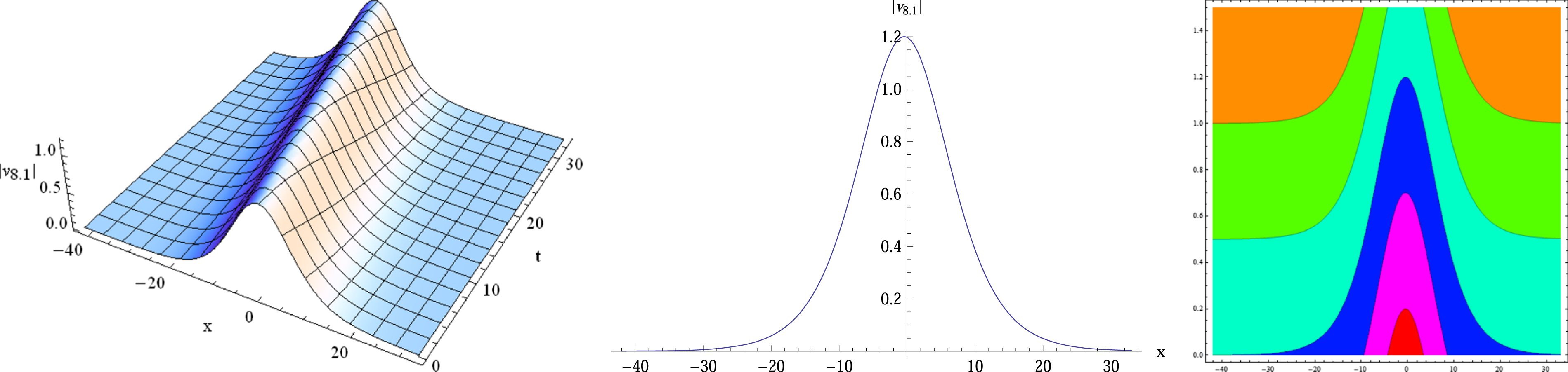
The 3D plot, 2D plot, and contour plot of
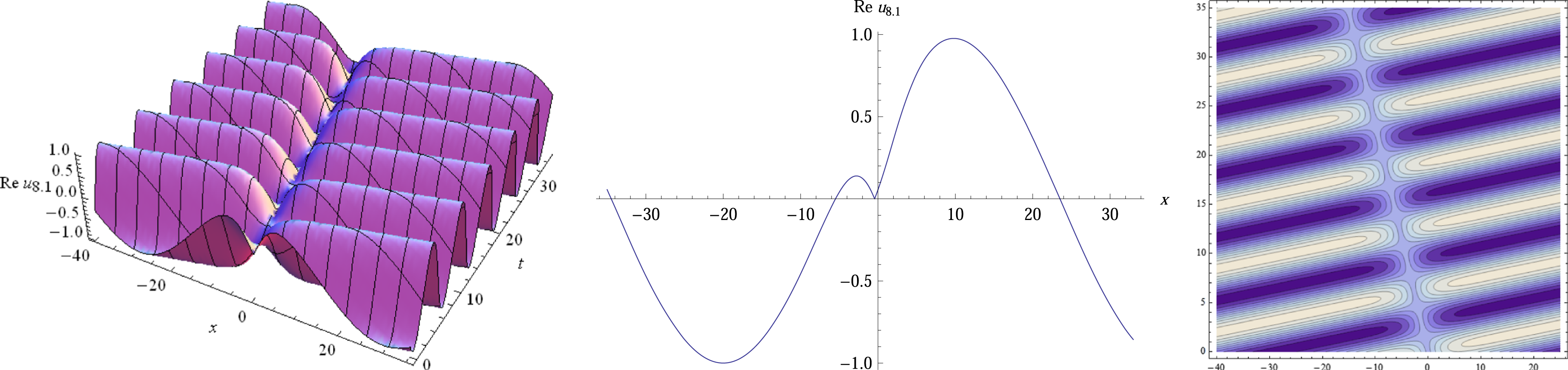
The 3D plot, 2D plot, and contour plot of
The 3D plot, 2D plot, and contour plot of
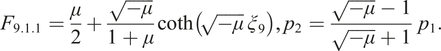
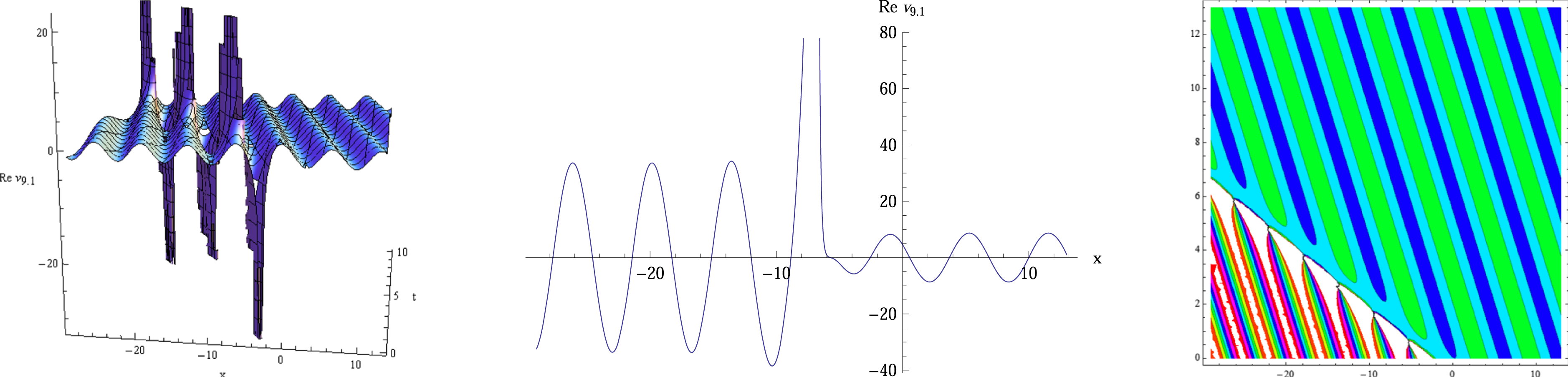
From case 2, we can deduce the traveling wave solution of equation (1) as follows
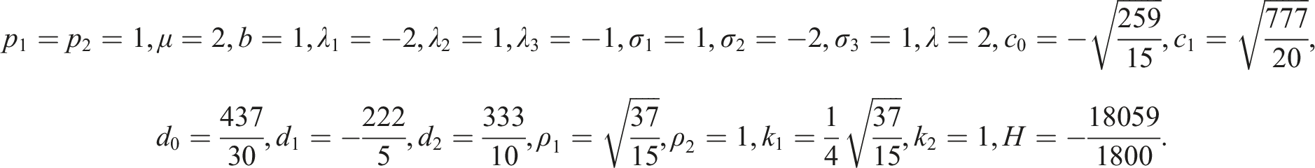
In this result, we can deduce the traveling wave solution of equation (1) as follows Selecting the following parameters in Selecting the following parameters in


The 3D plot, 2D plot, and contour plot of
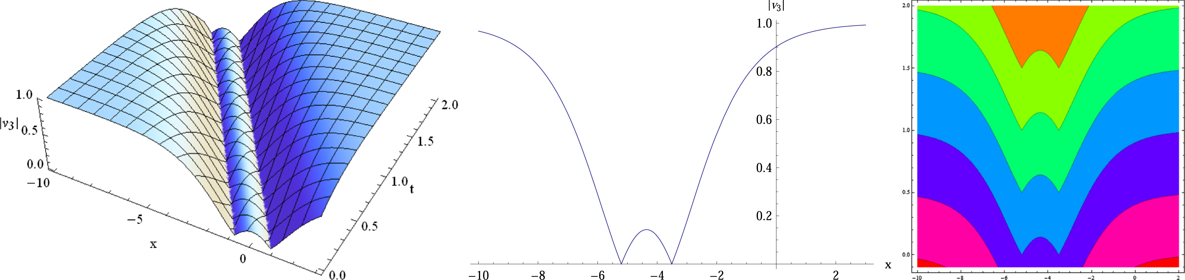
The W-shaped pulse solutions’ 3D plot, 2D plot, and contour plot of
From case 4, we have The blow-up pulse solution
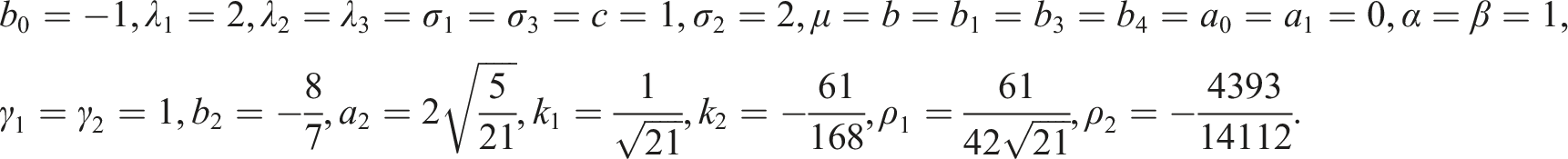
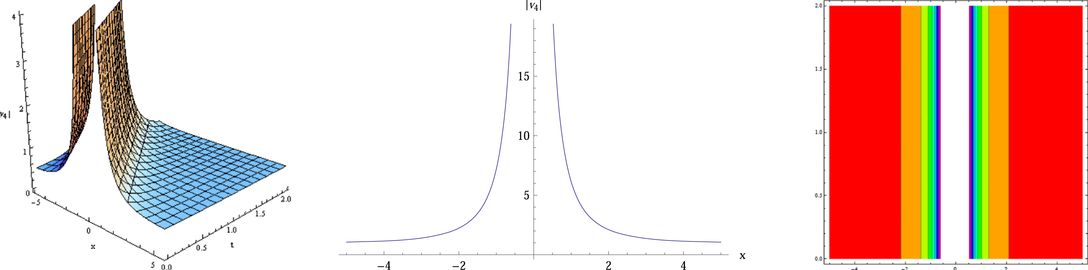
The blow-up pulse solutions’ 3D plot, 2D plot, and contour plot of
If we let
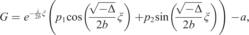
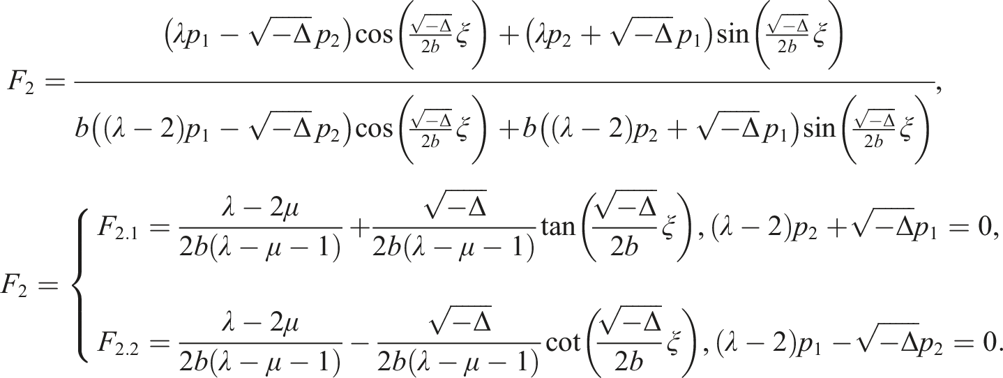
In this situation, we produce the following solutions of the above AEs.
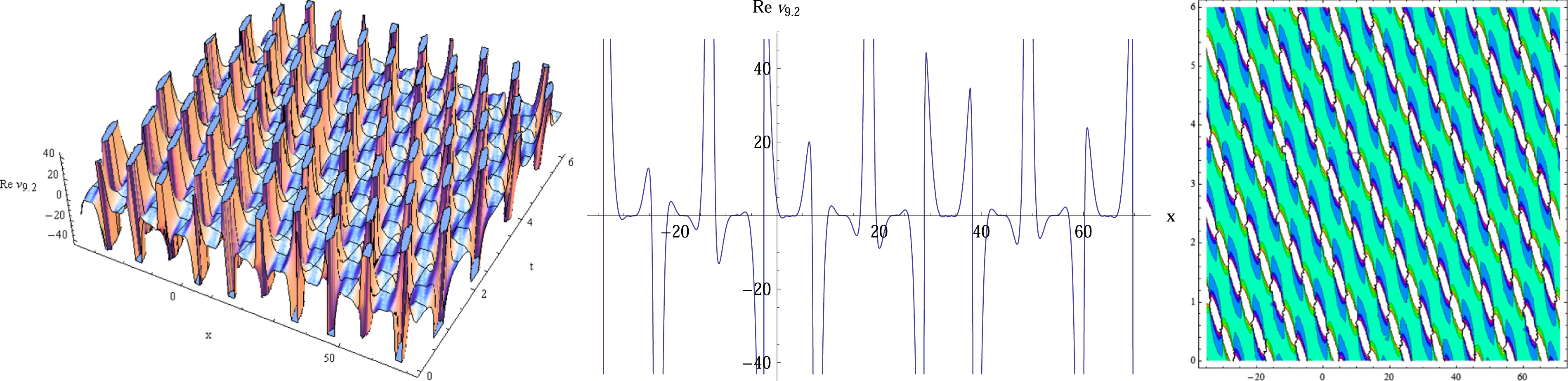
From (9), (13), (14), and (17), we can deduce the traveling wave solution of equation (1) as follows If we select the following parameters, the periodic pulse solutions can be simulated in Figures 7 and 8. Obviously, the solution


The periodic pulse solutions’ 3D plot, 2D plot, and contour plot of
The 3D plot, 2D plot, and contour plot of
If we let
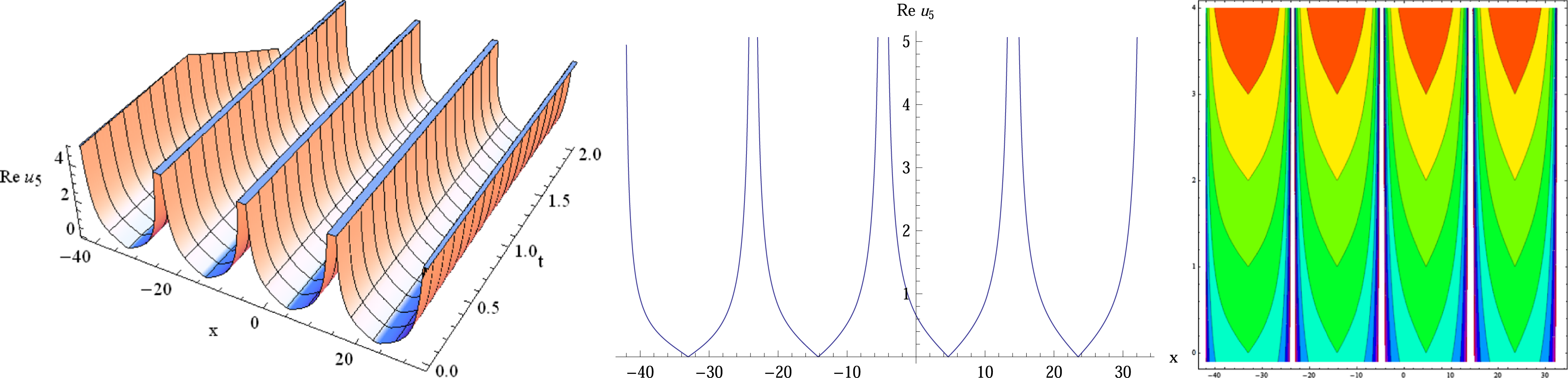
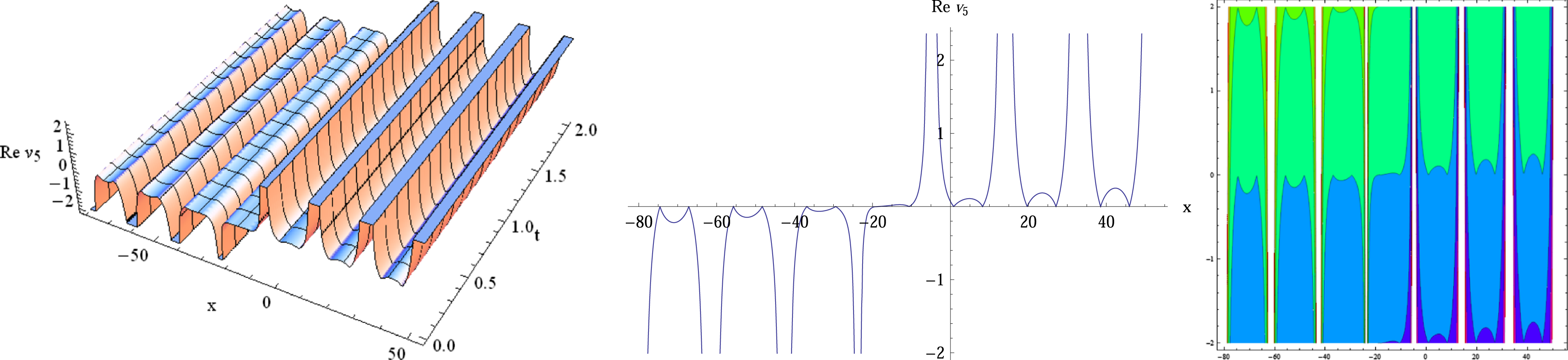
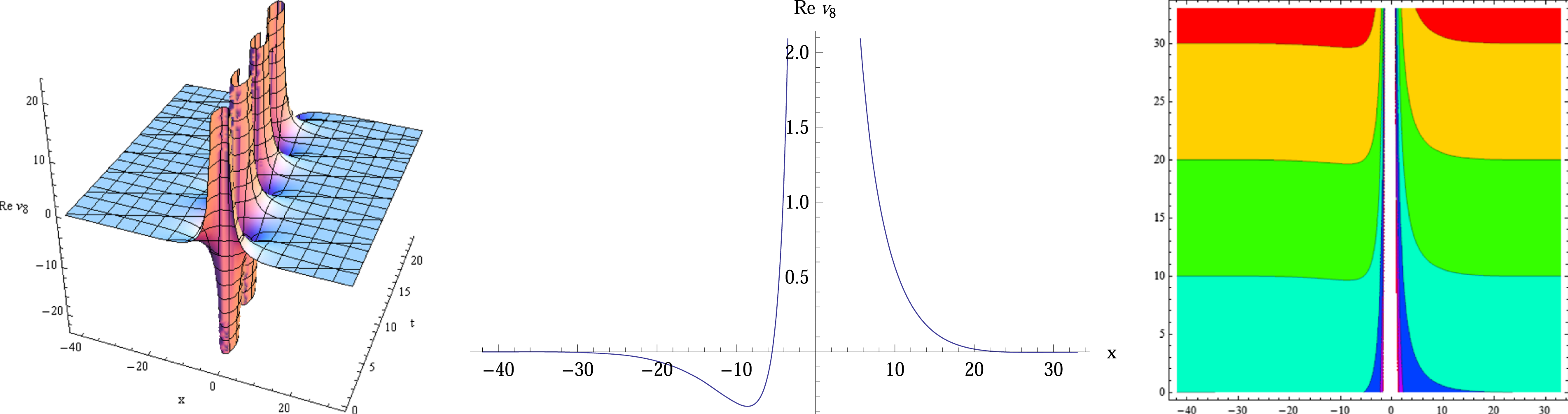
In this result, we have Thus The singular trigonometric function wave pulse can be simulated in Figure 9 by selecting
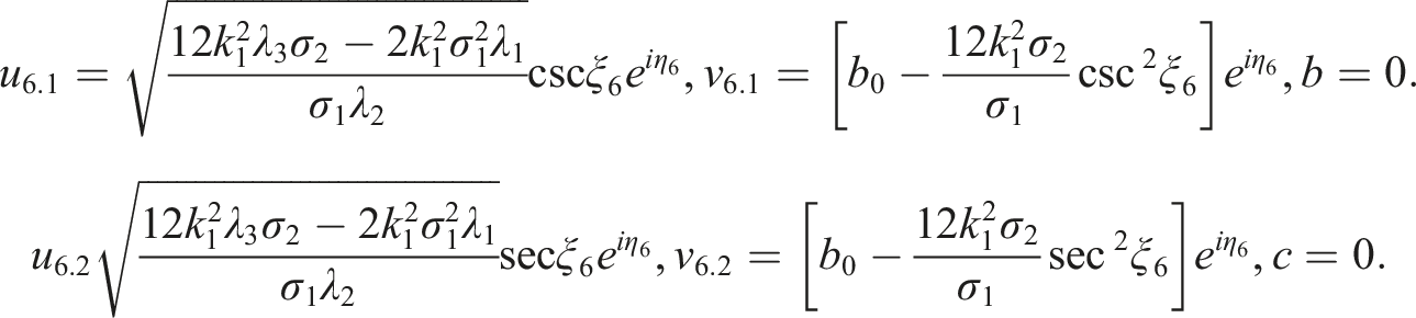


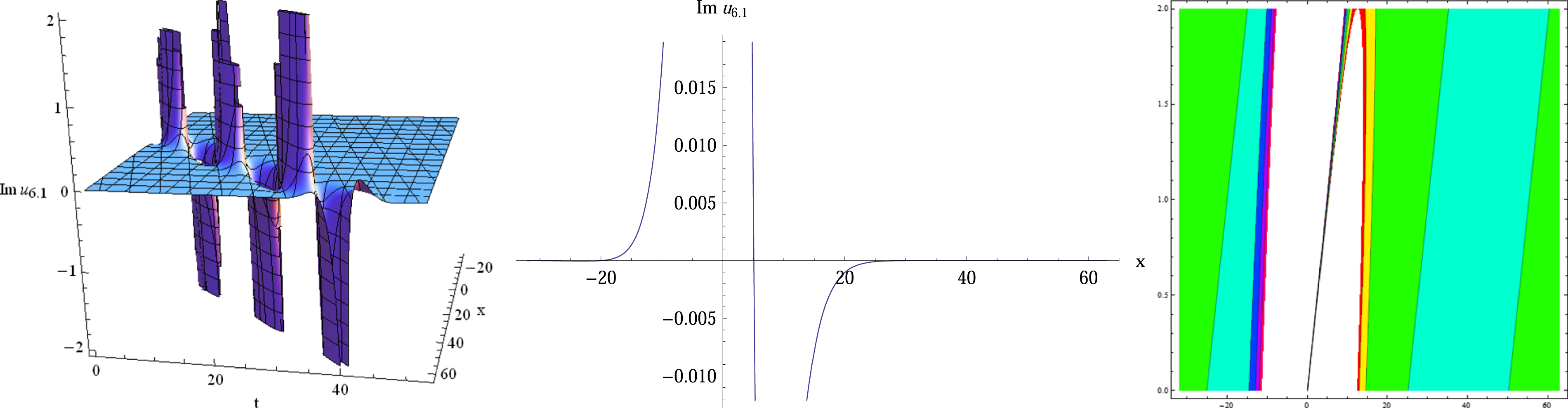
The 3D plot, 2D plot, and contour plot of the singular wave pulse
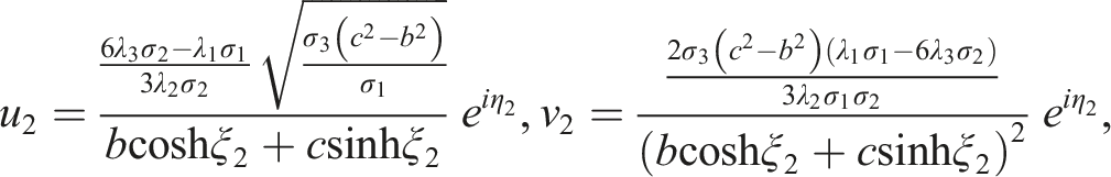
From case 3, we obtain In the following, let us consider the Gʹ/(bGʹ + G + a) method, we assume equation (16) have the following solutions Substituting equations (18) and (12) into equation (16) and setting the coefficients of After solving the AEs along with equations (13) and (14), we can get the following solutions
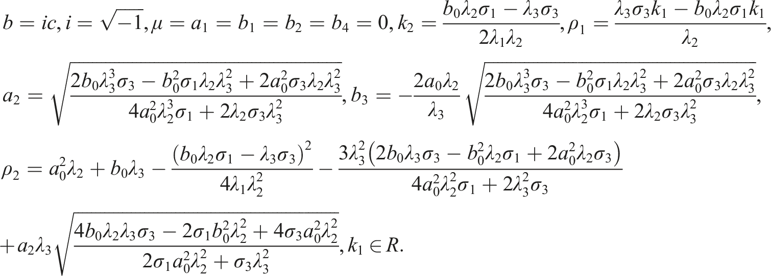
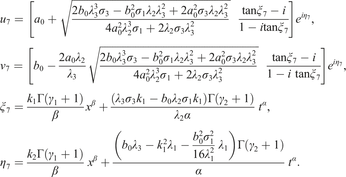

From case 1, we can determine the following solutions The singular solitary wave pulse and classical bell-shape bright soliton pulse are simulated in Figures 10–13 after selecting In particular, by selecting different From case 2, we get When If selecting We obtain the unbounded solitary wave solution When If we select Thus, the unbounded periodic wave solution We can easily find that


The 3D plot, 2D plot, and contour plot of the singular wave pulse
The 3D plot, 2D plot, and contour plot of the solitary wave pulse
The 3D plot, 2D plot, and contour plot of the famous bell-shape soliton pulse
The 3D plot, 2D plot and contour plot of
The 3D plot, 2D plot, and contour plot of
The 3D plot, 2D plot, and contour plot of
Results and discussion
After utilizing the two methods, we get many types of exact solutions of equation (1), including the bell-shape bright soliton pulse solution, the kink and anti-kink dark soliton pulse solution, the blow-up pattern solution, the W-shape soliton solution, the mixed solitary wave pattern solution, the periodic wave solution, etc. Some structures of these solutions are simulated in Figures 1–15. The visualization can help us to better understand the dynamic behavior, physical, and propagation characteristics of the coupled model. For example, by selecting The change of real part for 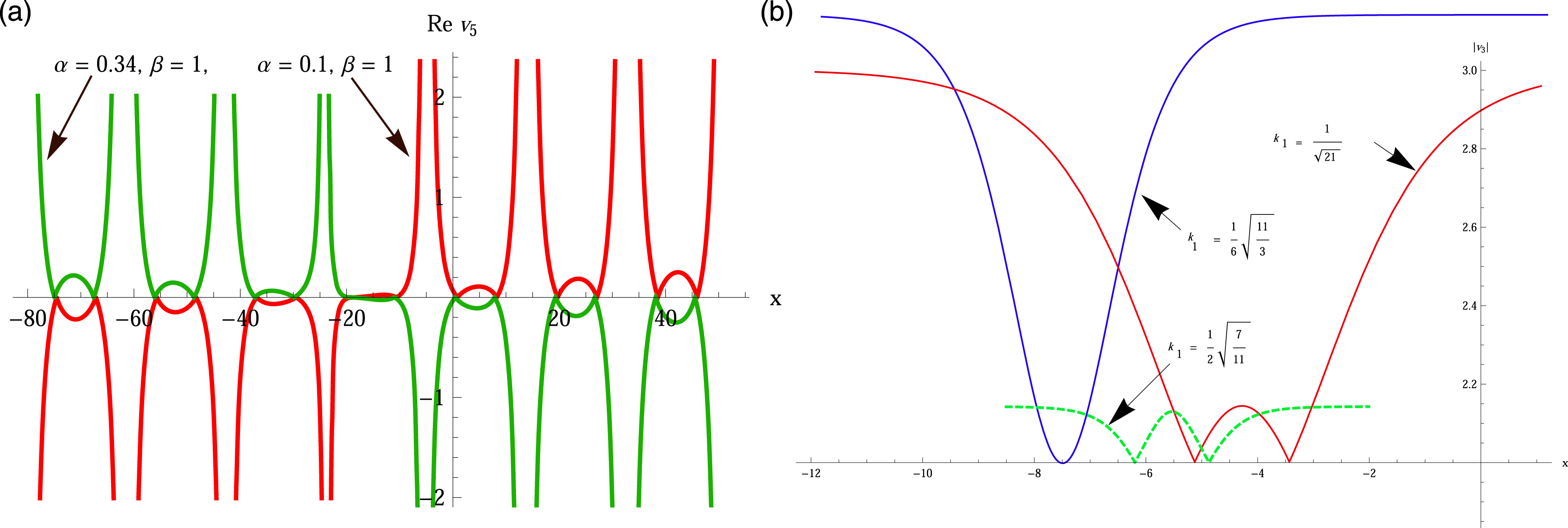
All of the nine types of solutions and parameter values obtained in this paper have been checked by mathematica software, and they are found for the first time to our knowledge.
Conclusion
In conclusion, nine types of new exact solutions for the MFCNLS-KdV have been found after utilizing the modified (Gʹ/G, 1/G) and Gʹ/(bGʹ + G + a) methods. Some propagation behavior of these solutions are discussed and simulated, the graphs of which shows that these solitary wave solutions and periodic solutions are propagated through different pattern, these patterns are important for revealing the internal structure of equation (1), the efficient and significant methods can be used to many other nonlinear models such as Hirota–Satsuma KdV equation, Ginzburg–Landau equation, Boussinesq–Burgers equation, etc. The current definition of M-fractional derivatives still has great limitations, and it is difficult to characterize the necessary connection between two real number order derivatives. On the other hand, the unified definition of fractional derivatives needs to be further explored and developed for us in the future. Finally, all simulations of these solutions obtained in the present article have been checked by the mathematica software.
Footnotes
Declaration of conflicting interests
The author(s) declared no potential conflicts of interest with respect to the research, authorship, and/or publication of this article.
Funding
The author(s) disclosed receipt of the following financial support for the research, authorship, and/or publication of this article: Project was partially supported by Jiangsu university students practical innovation training program guidance project of Jiangsu Province (Grant No. 202211276054Y), Natural science research projects of Institutions of higher learning in Jiangsu Province (Grant No. 18KJB110013) and Nanjing Institute of Technology (Grant No. CKJB201709).
CRediT authorship contribution statement
Baojian Hong: Completed all of the study, carried out the results of this article and drafted the paper.
Availability of data and material
The author affirmed availability of data and material in deriving the solutions mentioned in this manuscript.