Sage Journals: Discover world-class research

Abstract

Previously, it was shown how the behavior of chain-like structures including hysteretic elements as described by the Bouc model under white noise excitation can be calculated using Gaussian closure. The method results in analytic expressions for the temporal evolution of the statistical moments. Using the example of a liquid-filled tank, the Gaussian closure is generalized to the case of a filtered white noise with a slowly varying intensity as may occur during earthquakes. The complexity of the model is further enhanced for a case that lacks an elastic restoring force at the hysteretic node that couples the tank model with the surface. The new tank model comprises three mechanical degrees of freedom. The first degree of freedom is the movement of mass of the tank. The second degree of freedom is the movement of the swapping mass of the fluid in the tank. The third degree of freedom is the movement of the impulsive mass that is coupled more stiffly.

Keywords

Gaussian closure technique Bouc hysteretic model random vibration

Introduction

In the event of an earthquake, tanks with liquids suffer from the large forces induced by the horizontal component of the ground acceleration. A potential way to reduce the forces acting on the tank is by means of hysteretic springs for which the reduction is caused by three effects.¹ The first is the limitation of the stresses in the tank caused by the stress limit of the hysteretic element. The second is that no resonance amplification is given due to the non-linearity of the hysteretic spring. The third is the damping effect of the hysteresis.

The non-linear behavior of such hysteretic systems can be described by Bouc’s model² or its extension, the Bouc–Wen model.^3–11 Further extensions introducing degradation are added by Baber and Noori.¹² This model describes a hysteresis as it can be found in various materials, for example, rubber, steel, and concrete.¹ Other models as an alternative to the Bouc hysteresis also exist such as a bi-linear hysteresis is described by Suzuki and Minai.¹³ Aloisio et al.¹⁴ present an overview about modified versions of the Bouc–Wen model and the Suzuki–Minai model.

The state-of-the-art approaches to determine the response of a hysteretic system under stochastic excitation are either the usage of Monte Carlo simulations which can be applied to any type of hysteretic models,¹ and the classical statistical linearization is appropriate for the estimation of the stationary response^6,15,16 or there exists also a time-dependent response using a time step procedure.¹⁷

A new approach is the stochastic elastic-plastic finite elements based on the Fokker–Planck equation that are used by Sett et al.¹⁸ where also a detailed theory of elastic-plastic behavior is given. Briefly, the new approach can be used to deal with randomness of the elastic-plastic parameters. Random fields are discretized by means of the Karhunen–Loeve expansion¹⁹ and the polynomial chaos¹⁹ is used to derive orthogonal moment equations from the random variables. A difficulty of the proposed method is the large number of unknown coefficients, if higher-order moments are used. Further approaches include a path integration method based on the Fokker–Planck equation presented in Narayanan and Kumar²⁰ and the probability density evolution method described in Li and Chen.²¹ In the latter, a bi-linear hysteresis is used for the elastic-plastic behavior. The hysteresis consists of a stiffer elastic part and a softer plastic part. Thus, the behavior has also an elastic component in the plastic region.

A different approach for hysteretic systems under stochastic excitation is the Gaussian closure.^22–25 Previously²⁶, a non-linear parametric model for the sloshing mass of a tank was presented and solved by means of the Gaussian closure technique. Compared to the hysteretic system, this was less complex as the non-linearity was of polynomial type. Such a non-linearity leads to classical moments of higher order that are handled by Isserlis’ theorem^27,28 which is not possible for a hysteretic spring. Still, for the Bouc model and some special cases of the Bouc–Wen model, the Gaussian closure can be solved analytically even in the hysteretic case. Furthermore, compared to linearization approaches, the advantage of the Gaussian closure method is that it allows the derivation of analytic solutions for the moments at every time step of the transient simulation.^1,29 This property was also shown for chain-like multiple degree-of-freedom (MDOF) systems when no dead load is present.²⁴

The motivation of the work presented here is to find a method for a non-linear MDOF mechanical system under colored time-dependent noise excitation which is a typical setting for earthquake events for which the behavior of tanks with an elastic-plastic support is especially critical. The use of the Gaussian closure allows for an almost analytical solution in every time step. The derivation of an analytic solution assuming a multivariate Gaussian distribution for every time step is limited to the Bouc model and is not possible for either the Bouc–Wen model or the bi-linear Suzuki–Minai model.

The model of the tank used here is a special case of an MDOF model described in Waubke²⁴ based on the Bouc model.² It is assumed that the tank is rigid and placed on hysteretic elements, that is, only the coupling of the tank with the ground is realized with a hysteretic spring. The tank itself comprises two further linearly coupled mechanical degrees of freedom. In addition to the mass of the tank, two masses are coupled to the tank: a sloshing mass with a low resonance frequency and an impulsive mass with a high resonance frequency. Usually, the impulsive mass is added to the tank mass and the system is reduced to two mechanical degrees of freedom, whereas here it is assumed that the impulsive mass is coupled in a stiffer way to the tank than the sloshing mass.^30–35

Thus far, the usage of the Gaussian closure technique is limited either to the SDOF case with the transient response to a time-dependent loading and a dead load²⁹ or the MDOF case with a symmetric stationary white noise load.²⁴

Here, the features of the SDOF model will be extended to the MDOF case. The Gaussian closure is based on the state vector differential equation using the scheme that was already presented^23–25, but in the current work, a dead load is included. Thus, a shift value for the hysteretic stress z₀ had to be added. This value can be used to simulate a downhill drift caused by the vertical component of the earthquake event. This leads to a shifted Gaussian distribution. Therefore, the mean values have to be derived additionally to the covariances, and the equations derived for the Gaussian closure method become much more complex.

No viscose damping and linear stiffness are assumed, that is, the linear part of the spring at the base is set to zero. The calculation of a stationary response is no more possible, as the variance of the displacement of the tank tends to infinity for a stationary load.

Earthquakes are typically short events with a wide band frequency content. Therefore, as a novelty a time-dependent colored noise will be included in the model which is achieved by processing the white noise with a filter described by a second order differential equation added to the state vector of the mechanical system. The limited duration is simulated using a time window that reduces slowly the amplitude of the white noise process.

For the model described above, different settings and approaches were investigated. First, an analytic solution for the Gaussian closure is only possible, if the hysteretic springs are defined in relative coordinates. Linear springs, in contrast, can be defined in absolute or relative coordinates. For the latter, both possibilities were tested.

Second, the evolution of the moments can be simulated using a simple time step procedure (see, e.g., Waubke²⁴) using the derivative of the moments with respect to time. In addition to this simple approach, the explicit Runge–Kutta method and the implicit Radau method were also implemented and tested.

The different settings used in the Gaussian closure were compared with the Monte Carlo simulation as the state-of-the-art method. The Monte Carlo simulation was based on the same state vector equation as in the Gaussian closure method and uses the same time step procedures for every realization of the process. The step size of the iterations with respect to time is also the same.

In the following chapters, the main steps for the derivation of the moment equations are presented, the stability of the equations is tested, and results from the Gaussian closure are compared to the results from the Monte Carlo simulation.

Multi-degree of freedom model of a tank

In the proposed model, the tank is rigid and placed on hysteretic elements (Figure 1). The liquid is modeled by a sloshing and an impulsive mass which is assumed to be linearly coupled with the tank. For this case, a simple description in relative coordinates is possible. The excitation is given by a ground acceleration, as it is given by earthquakes or high level vibration. To achieve such an excitation, Gaussian white noise is sent through a differential filter of the second order that acts as a low-pass filter.

Figure 1.

The model of the tank with tank mass m_t, sloshing mass m_s, and impulsive mass m_i. The viscose dampers are c_t, c_s, and c_i. The linear springs are k_s and k_i. The hysteretic element is k_t. The force z₀ · k_t is, caused by a downhill drift.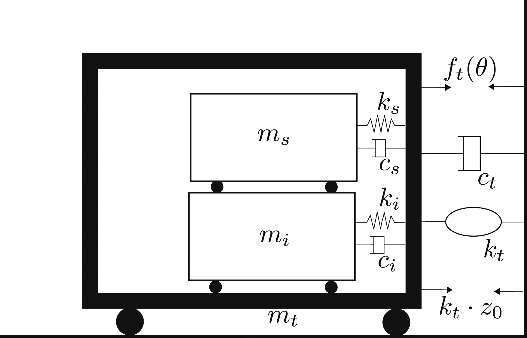

The index f is used for the filter parameters (m_f, c_f, and k_f) filtering the white noise excitation. The output of the filter is the random excitation f_t(θ). The index s is used for the sloshing mass, damping, and stiffness parameters of the sloshing mass (m_s, c_s, and k_s). The index i is related to the impulsive mass (m_i, c_i, and k_i). In the same manner, the parameters of the tank are given (m_t, c_t, and k_t). The Bouc hysteresis is defined with the parameters A, γ, and θ. The participation factor between linear elastic and hysteretic support of the tank is given by α_t. The new parameter z₀ is the deterministic load on the tank. The white noise excitation of the filter is defined by ξ_f and the intensity by K_f. The Bouc model in the classical and in a modified form are given in equation (1)

\frac{\partial}{\partial t} z_{t} = A v_{t} - γ | v_{t} | z_{t} + θ v_{t} | z_{t} | = A v_{t} - v_{t} z_{t} (γ sgn (v_{t}) + θ sgn (z_{t})) .

(1)

Initial calculations showed that the high resonance frequency of the impulsive mass together with the low frequency filter of the load may lead to difficulties in particular at high excitation noise levels because coherent behavior of state vector variables can occur. For very high levels of excitation, low level white noise processes on every degree of freedom stabilized the time step procedure. These white noise processes (for clarity, termed stabilizing noise) on the structure are defined by ξ_s, ξ_i, and ξ_t. 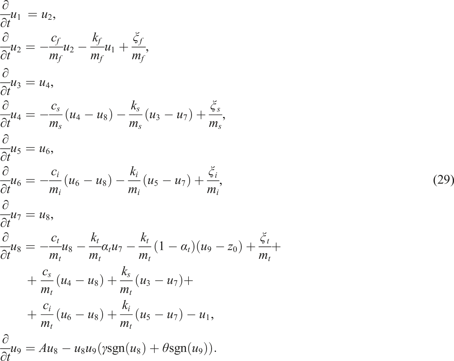The intensities are given by $K_{s} = K_{f} \frac{m_{s}^{2}}{10000} m_{f}^{2}, K_{i} = K_{f} \frac{m_{i}^{2}}{10000} m_{f}^{2}$ , and $K_{t} = \frac{K_{f} m_{t}^{2}}{10000} m_{f}^{2}$ . However, this additional noise leads to inaccuracies at lower levels of excitation. Possible solutions to this issue will be addressed in detail in the results section.

For a more general notation of the moment equation and the respective integrals, a state vector u is introduced in equation (2) with the following components. The displacement x_f of the ground and its derivative v_f, the jerk, is denoted as u₁ and its derivative u₂. The relative displacement x_s of the sloshing mass with respect to the tank and the corresponding velocity v_s is u₃ and u₄. The relative displacement of the impulsive mass x_i with respect to the tank and the corresponding velocity v_i are u₅ and u₆. The relative displacement x_t of the tank mass with respect to the ground vibration and the corresponding velocity v_f is u₇ and u₈. The force proportional displacement of the tank z_t is given by u₉. The deterministic load that can also be interpreted as a shift parameter that leads to a non-symmetry of the hysteresis is z₀. This leads to the set of equations given in equation (2)

\begin{array}{c} \frac{\partial}{\partial t} x_{f} = \frac{\partial}{\partial t} u_{1} = u_{2}, \\ \frac{\partial}{\partial t} v_{f} = \frac{\partial}{\partial t} u_{2} = - \frac{c_{f}}{m_{f}} u_{2} - \frac{k_{f}}{m_{f}} u_{1} + \frac{ξ_{f}}{m_{f}}, \\ \frac{\partial}{\partial t} x_{s} = \frac{\partial}{\partial t} u_{3} = u_{4}, \\ \frac{\partial}{\partial t} v_{s} = \frac{\partial}{\partial t} u_{4} = - \frac{c_{s}}{m_{s}} u_{4} - \frac{k_{s}}{m_{s}} u_{3} + \frac{ξ_{s}}{m_{s}} + \\ + \frac{c_{t}}{m_{t}} u_{8} + \frac{k_{t}}{m_{t}} α_{t} u_{7} + \frac{k_{t}}{m_{t}} (1 - α_{t}) (u_{9} - z_{0}) - \\ - \frac{c_{s}}{m_{t}} u_{4} - \frac{k_{s}}{m_{t}} u_{3} - \frac{c_{i}}{m_{t}} u_{6} - \frac{k_{i}}{m_{t}} u_{5}, \\ \frac{\partial}{\partial t} x_{i} = \frac{\partial}{\partial t} u_{5} = u_{6}, \\ \frac{\partial}{\partial t} v_{i} = \frac{\partial}{\partial t} u_{6} = - \frac{c_{i}}{m_{i}} u_{6} - \frac{k_{i}}{m_{i}} u_{5} + \frac{ξ_{i}}{m_{i}} + \\ + \frac{c_{t}}{m_{t}} u_{8} + \frac{k_{t}}{m_{t}} α_{t} u_{7} + \frac{k_{t}}{m_{t}} (1 - α_{t}) (u_{9} - z_{0}) - \\ - \frac{c_{s}}{m_{t}} u_{4} - \frac{k_{s}}{m_{t}} u_{3} - \frac{c_{i}}{m_{t}} u_{6} - \frac{k_{i}}{m_{t}} u_{5}, \\ \frac{\partial}{\partial t} x_{t} = \frac{\partial}{\partial t} u_{7} = u_{8}, \\ \frac{\partial}{\partial t} v_{t} = \frac{\partial}{\partial t} u_{8} = - \frac{c_{t}}{m_{t}} u_{8} - \frac{k_{t}}{m_{t}} α_{t} u_{7} - \frac{k_{t}}{m_{t}} (1 - α_{t}) (u_{9} - z_{0}) + \frac{ξ_{t}}{m_{t}} + \\ + \frac{c_{s}}{m_{t}} u_{4} + \frac{k_{s}}{m_{t}} u_{3} + \frac{c_{i}}{m_{t}} u_{6} + \frac{k_{i}}{m_{t}} u_{5} - u_{1}, \\ \frac{\partial}{\partial t} z_{t} = \frac{\partial}{\partial t} u_{9} = A u_{8} - u_{8} u_{9} (γ sgn (u_{8}) + θ sgn (u_{9})) . \end{array}

(2)

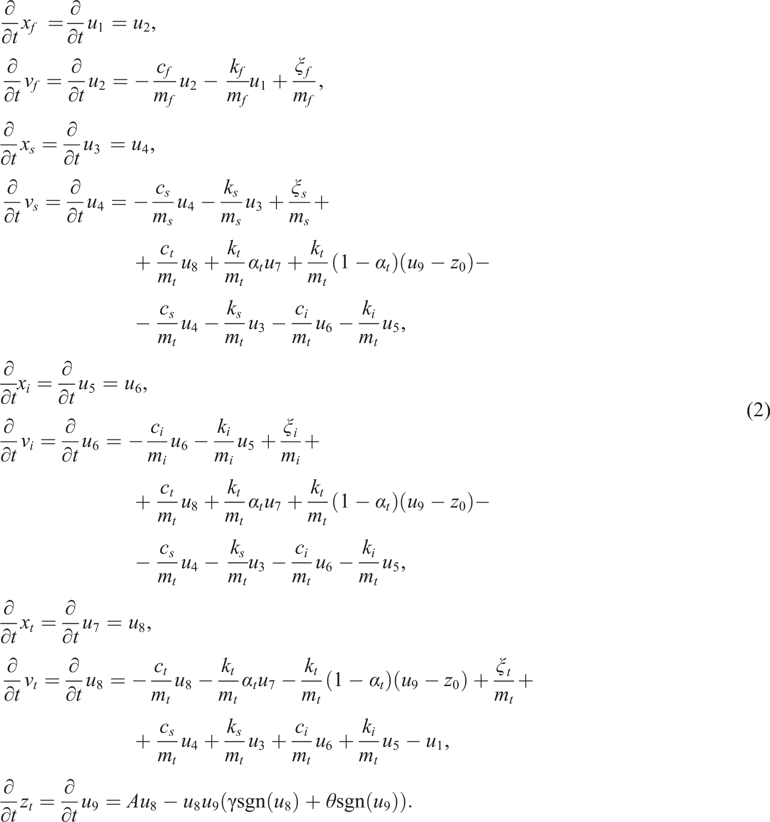
In the Monte Carlo simulation, the first order differential equations given above are solved using a simple time step procedure. An iteration is needed for the sgn function. First, the sign of the values u₈ and u₉ at the beginning of the interval is used. If the sign changes at the end of the interval, a second iteration with the sign at the end of the interval is used. If the sign at the end of the interval changes again, the sgn function is set to zero.

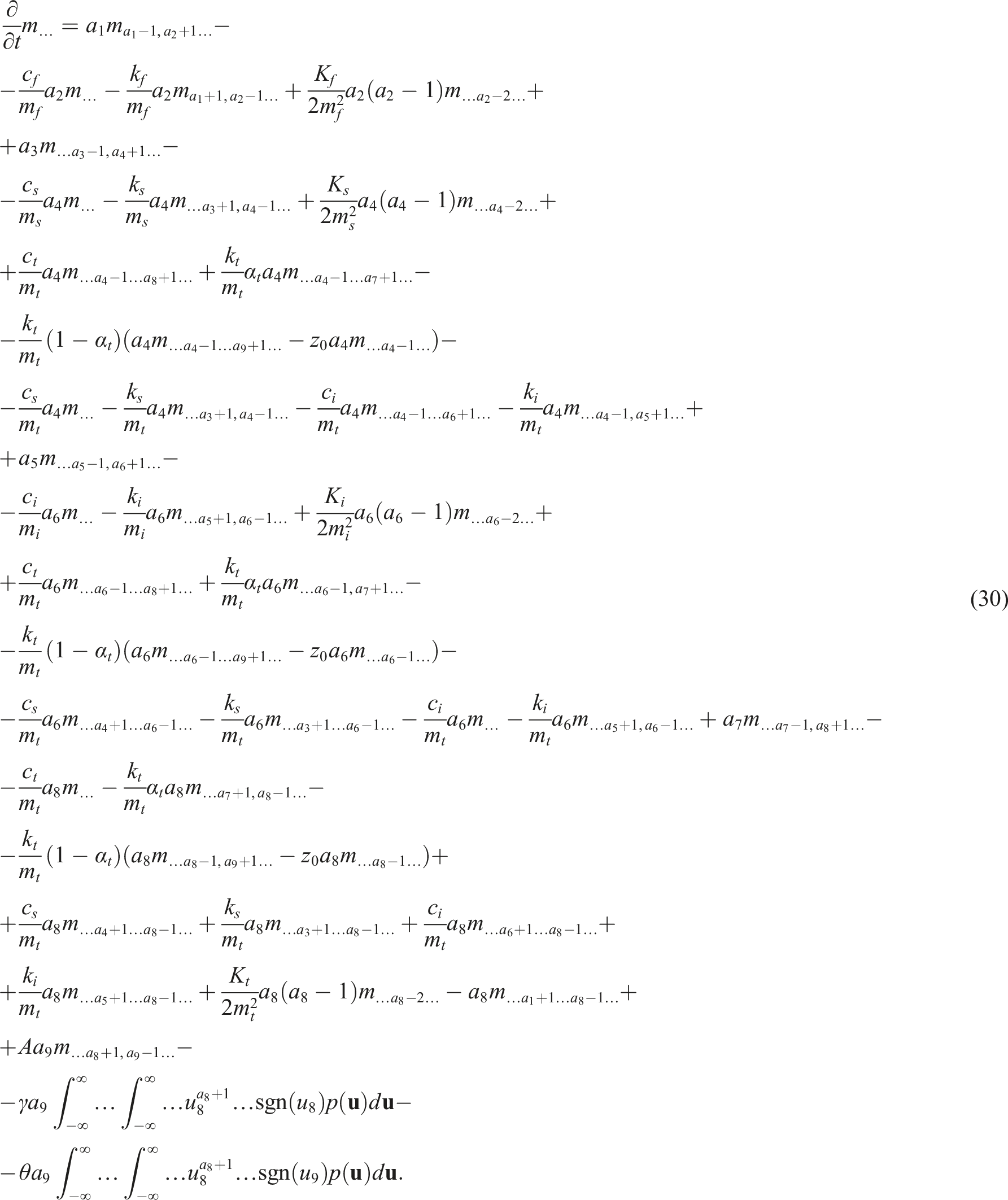
To derive moment equations, the related Fokker–Planck–Kolmogorov equation^1,22,36 is weighted by $E (\prod_{i} u_{i}^{a_{i}})$ . Only first and second order moments are derived. Therefore, the following relation holds 1 ≤ ∑_i a_i ≤ 2. If negative indexes occur in the moments, the moments are zero. If higher-order moments occur in the equations they are substituted by first and second order moments using Isserlis theorem^27,28 assuming a Gaussian distribution. Additionally, the moments including the (sgn) function are evaluated assuming a Gaussian distribution.

The moment equation for this case is given by

\begin{array}{l} \frac{\partial}{\partial t} m_{\dots} = a_{1} m_{a_{1} - 1, a_{2} + 1 \dots} - \\ - \frac{c_{f}}{m_{f}} a_{2} m_{\dots} - \frac{k_{f}}{m_{f}} a_{2} m_{a_{1} + 1, a_{2} - 1 \dots} + \frac{K_{f}}{2 m_{f}^{2}} a_{2} (a_{2} - 1) m_{\dots a_{2} - 2 \dots} + \\ + a_{3} m_{\dots a_{3} - 1, a_{4} + 1 \dots} - \\ - \frac{c_{s}}{m_{s}} a_{4} m_{\dots} - \frac{k_{s}}{m_{s}} a_{4} m_{\dots a_{3} + 1, a_{4} - 1 \dots} + \frac{K_{s}}{2 m_{s}^{2}} a_{4} (a_{4} - 1) m_{\dots a_{4} - 2 \dots} + \\ + \frac{c_{t}}{m_{t}} a_{4} m_{\dots a_{4} - 1 \dots a_{8} + 1 \dots} + \frac{k_{t}}{m_{t}} α_{t} a_{4} m_{\dots a_{4} - 1 \dots a_{7} + 1 \dots} - \\ - \frac{k_{t}}{m_{t}} (1 - α_{t}) (a_{4} m_{\dots a_{4} - 1 \dots a_{9} + 1 \dots} - z_{0} a_{4} m_{\dots a_{4} - 1 \dots}) - \\ - \frac{c_{s}}{m_{t}} a_{4} m_{\dots} - \frac{k_{s}}{m_{t}} a_{4} m_{\dots a_{3} + 1, a_{4} - 1 \dots} - \frac{c_{i}}{m_{t}} a_{4} m_{\dots a_{4} - 1 \dots a_{6} + 1 \dots} - \frac{k_{i}}{m_{t}} a_{4} m_{\dots a_{4} - 1, a_{5} + 1 \dots} + \\ + a_{5} m_{\dots a_{5} - 1, a_{6} + 1 \dots} - \\ - \frac{c_{i}}{m_{i}} a_{6} m_{\dots} - \frac{k_{i}}{m_{i}} a_{6} m_{\dots a_{5} + 1, a_{6} - 1 \dots} + \frac{K_{i}}{2 m_{i}^{2}} a_{6} (a_{6} - 1) m_{\dots a_{6} - 2 \dots} + \\ + \frac{c_{t}}{m_{t}} a_{6} m_{\dots a_{6} - 1 \dots a_{8} + 1 \dots} + \frac{k_{t}}{m_{t}} α_{t} a_{6} m_{\dots a_{6} - 1, a_{7} + 1 \dots} - \\ - \frac{k_{t}}{m_{t}} (1 - α_{t}) (a_{6} m_{\dots a_{6} - 1 \dots a_{9} + 1 \dots} - z_{0} a_{6} m_{\dots a_{6} - 1 \dots}) - \\ - \frac{c_{s}}{m_{t}} a_{6} m_{\dots a_{4} + 1 \dots a_{6} - 1 \dots} - \frac{k_{s}}{m_{t}} a_{6} m_{\dots a_{3} + 1 \dots a_{6} - 1 \dots} - \frac{c_{i}}{m_{t}} a_{6} m_{\dots} - \frac{k_{i}}{m_{t}} a_{6} m_{\dots a_{5} + 1, a_{6} - 1 \dots} + a_{7} m_{\dots a_{7} - 1, a_{8} + 1 \dots} - \\ - \frac{c_{t}}{m_{t}} a_{8} m_{\dots} - \frac{k_{t}}{m_{t}} α_{t} a_{8} m_{\dots a_{7} + 1, a_{8} - 1 \dots} - \\ - \frac{k_{t}}{m_{t}} (1 - α_{t}) (a_{8} m_{\dots a_{8} - 1, a_{9} + 1 \dots} - z_{0} a_{8} m_{\dots a_{8} - 1 \dots}) + \\ + \frac{c_{s}}{m_{t}} a_{8} m_{\dots a_{4} + 1 \dots a_{8} - 1 \dots} + \frac{k_{s}}{m_{t}} a_{8} m_{\dots a_{3} + 1 \dots a_{8} - 1 \dots} + \frac{c_{i}}{m_{t}} a_{8} m_{\dots a_{6} + 1 \dots a_{8} - 1 \dots} + \\ + \frac{k_{i}}{m_{t}} a_{8} m_{\dots a_{5} + 1 \dots a_{8} - 1 \dots} + \frac{K_{t}}{2 m_{t}^{2}} a_{8} (a_{8} - 1) m_{\dots a_{8} - 2 \dots} - a_{8} m_{\dots a_{1} + 1 \dots a_{8} - 1 \dots} + \\ + A a_{9} m_{\dots a_{8} + 1, a_{9} - 1 \dots} - \\ - γ a_{9} \int_{- \infty}^{\infty} \dots \int_{- \infty}^{\infty} \dots u_{8}^{a_{8} + 1} \dots s g n (u_{8}) p (u) d u - \\ - θ a_{9} \int_{- \infty}^{\infty} \dots \int_{- \infty}^{\infty} \dots u_{8}^{a_{8} + 1} \dots s g n (u_{9}) p (u) d u . \end{array}

(3)

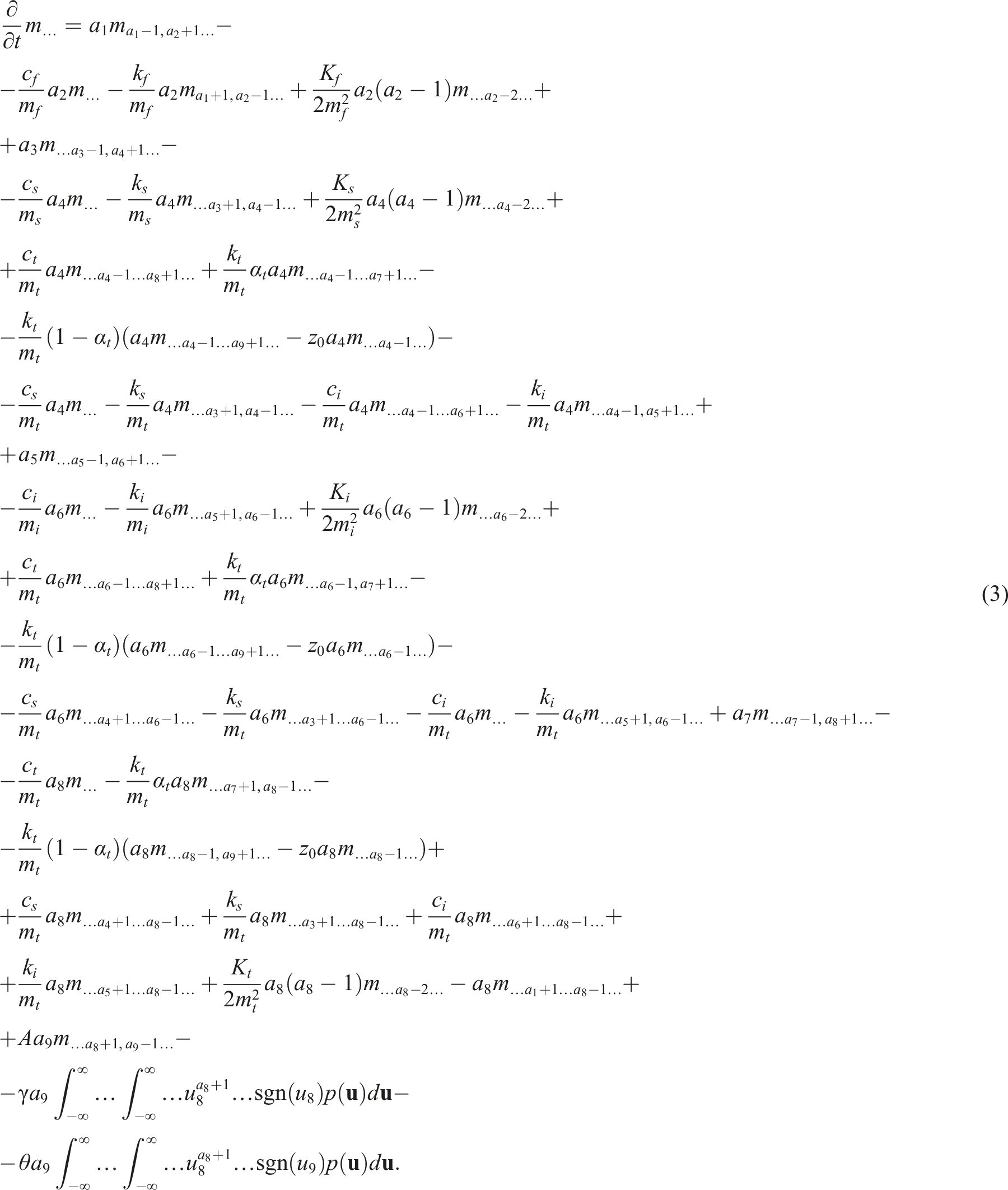
This expression can be used for a simple single time step procedure or for the multiple time step explicit Runge–Kutta RK4 or the adaptive implicit Radau algorithm. The Radau method has an accuracy estimate for the relative and absolute error. Both are set to 10⁻⁶. In equation (3), p(u) is the joint probability density of the state vector u. For the Gaussian closure, p(u) is a multivariate normal distribution of dimension s = 9 with the mean μ and the covariance matrix V

p (u) = \frac{1}{\sqrt{{(2 π)}^{s} | V |}} e^{- \frac{1}{2} {(u - μ)}^{T} V^{- 1} (u - μ) .}

(4)

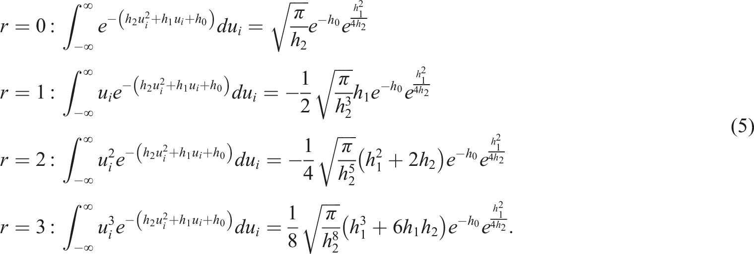
For the integrals without a sgn() function, the following relation is given for a weighting with $u_{i}^{r}$

\begin{array}{l} r = 0 : \int_{- \infty}^{\infty} e^{- (h_{2} u_{i}^{2} + h_{1} u_{i} + h_{0})} d u_{i} = \sqrt{\frac{π}{h_{2}}} e^{- h_{0}} e^{\frac{h_{1}^{2}}{4 h_{2}}} \\ r = 1 : \int_{- \infty}^{\infty} u_{i} e^{- (h_{2} u_{i}^{2} + h_{1} u_{i} + h_{0})} d u_{i} = - \frac{1}{2} \sqrt{\frac{π}{h_{2}^{3}}} h_{1} e^{- h_{0}} e^{\frac{h_{1}^{2}}{4 h_{2}}} \\ r = 2 : \int_{- \infty}^{\infty} u_{i}^{2} e^{- (h_{2} u_{i}^{2} + h_{1} u_{i} + h_{0})} d u_{i} = - \frac{1}{4} \sqrt{\frac{π}{h_{2}^{5}}} (h_{1}^{2} + 2 h_{2}) e^{- h_{0}} e^{\frac{h_{1}^{2}}{4 h_{2}}} \\ r = 3 : \int_{- \infty}^{\infty} u_{i}^{3} e^{- (h_{2} u_{i}^{2} + h_{1} u_{i} + h_{0})} d u_{i} = \frac{1}{8} \sqrt{\frac{π}{h_{2}^{8}}} (h_{1}^{3} + 6 h_{1} h_{2}) e^{- h_{0}} e^{\frac{h_{1}^{2}}{4 h_{2}}} . \end{array}

(5)

Using this relation, the following recursion for the n-dimensional case can be derived. First, the centered moments are derived from the uncentered moments calculated by the moment equations

V (u_{i} u_{j}) = E (u_{i} u_{j}) - E (u_{i}) \cdot E (u_{j}), i = 1 \dots s, j = i \dots s .

(6)

The integration with respect to the variable, where the sgn() function is given is sorted to the end of the integration sequence

I_{1,2} = \frac{1}{\sqrt{{(2 π)}^{s} | V |}} \int_{- \infty}^{\infty} \dots \int_{- \infty}^{\infty} q_{0} (u) sgn (u_{s}) e^{- \frac{1}{2} {(u - μ)}^{T} V^{- 1} (u - μ)} d u_{1} \dots d u_{s} .

(7)

The integral is reordered to simplify the integration procedure

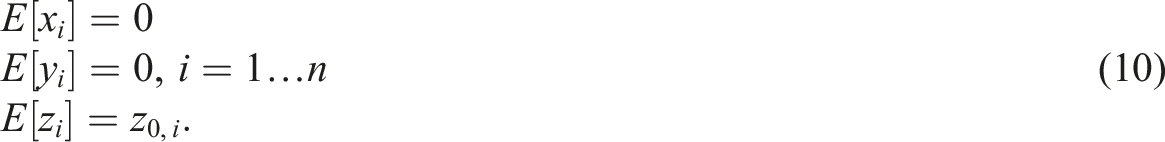
\begin{array}{c} I_{1,2} = \frac{1}{\sqrt{{(2 π)}^{s} | V |}} \int_{- \infty}^{\infty} \dots \int_{- \infty}^{\infty} q_{0} (u) sgn (u_{s}) \cdot \\ e^{- (\sum_{i = 1}^{s} \sum_{j = i}^{s} β_{i j, 0} u_{i} u_{j} + \sum_{i = 1}^{s} κ_{i, 0} u_{i} + ϵ_{0})} d u_{1} \dots d u_{s} . \end{array}

(8)

At the beginning of the time step procedure, the covariance matrix V is set to

V = diag {10^{- 8}}

(9)

This is necessary because the algorithm assumes a Gaussian distribution and cannot handle Dirac delta distributions that occur, if variables become deterministic. The mean values are set to zero with the exception of the mean values of the force proportional displacements z_i that are set to the shift value z_0,i

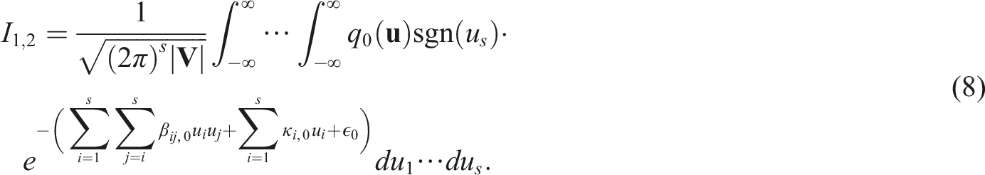
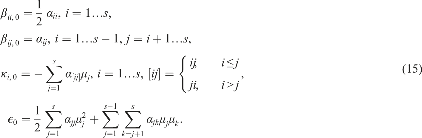
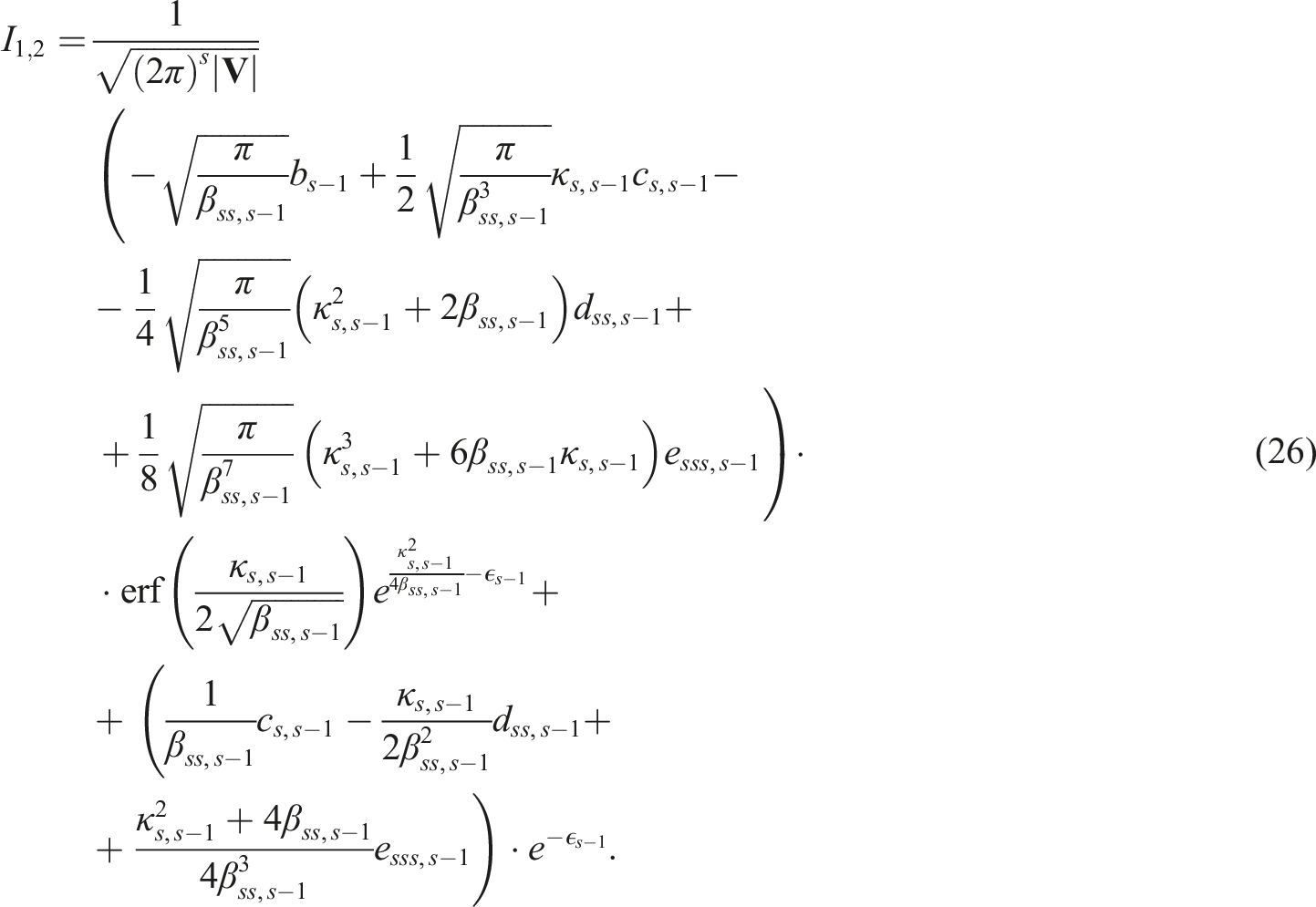
\begin{array}{l} E [x_{i}] = 0 \\ E [y_{i}] = 0, i = 1 \dots n \\ E [z_{i}] = z_{0, i} . \end{array}

(10)

The integral consists of an exponential function and a polynomial that can have exponents up to the third order for the first and second order moments needed for the Gaussian closure. A general description is possible by

q_{0} (u) = b_{0} + \sum_{i = 1}^{s} c_{i, 0} u_{i} + \sum_{i = 1}^{s} \sum_{j = i}^{s} d_{i j, 0} u_{i} u_{j} + \sum_{i = 1}^{s} \sum_{j = i}^{s} \sum_{k = j}^{s} e_{i j k, 0} u_{i} u_{j} u_{k} .

(11)

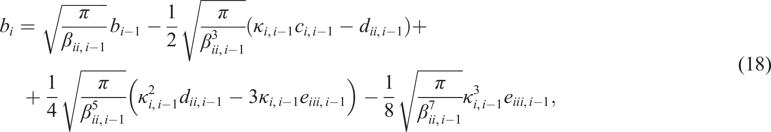
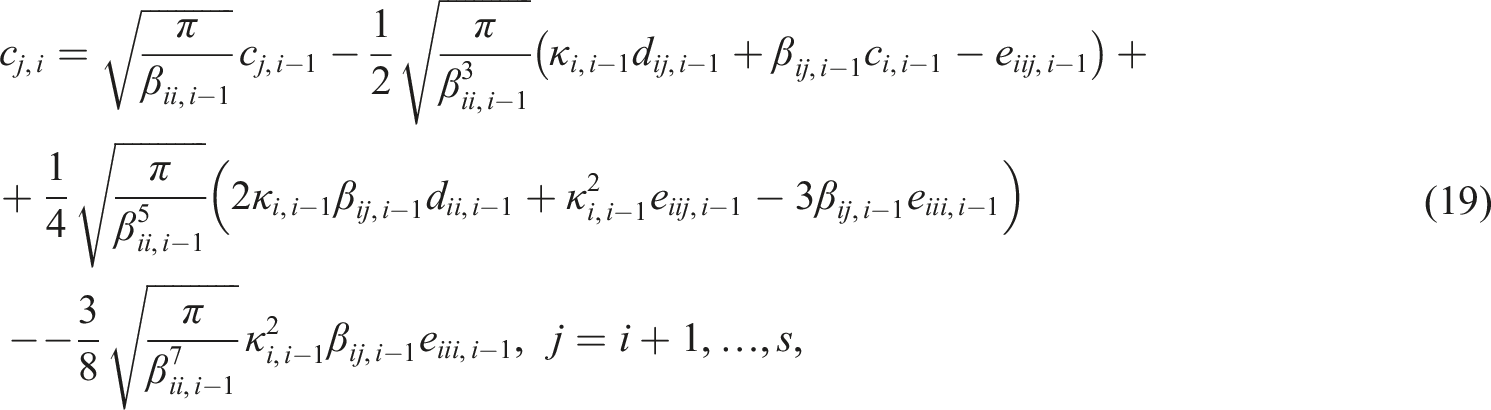
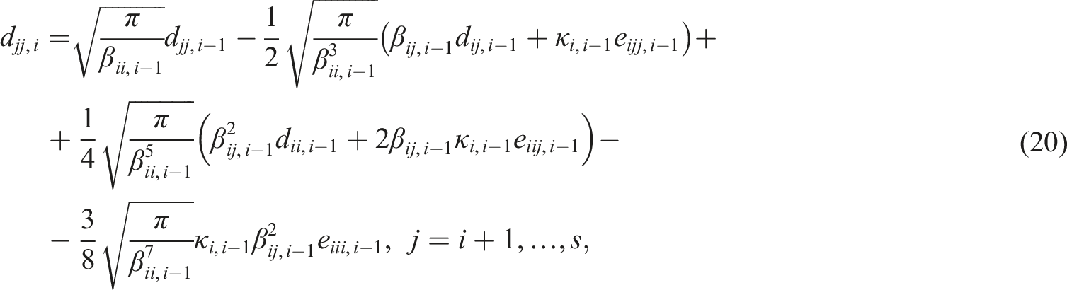
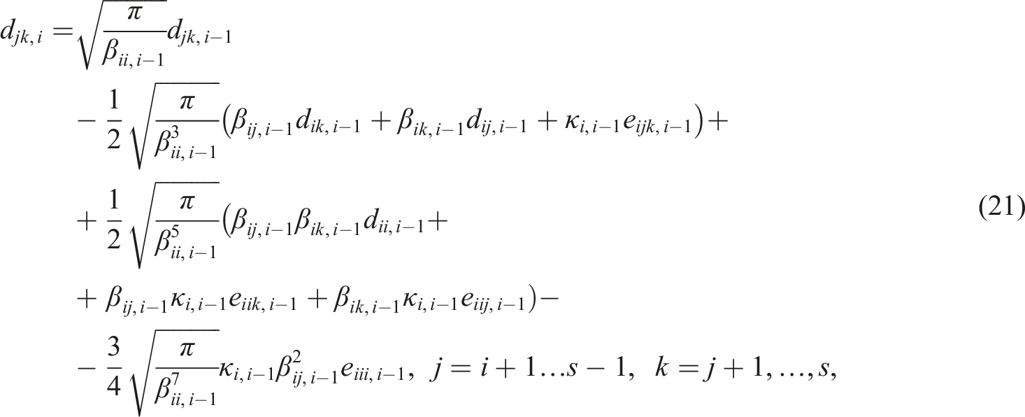
The coefficients b₀, c_i,0, d_ij,0, and e_ijk,0 are set to the given values of the polynomial in the integral I_1,2i. Usually only one coefficient is non-zero. Now the iteration about all dimensions of the state vector starts. In every step of the iteration, it is checked, whether the determinant of the covariance matrix is non-singular. To avoid a division by zero error, the determinant is limited to

| V | = \max {| V |, 10^{- 8}} .

(12)

The inverse is calculated by a generalized QR algorithm.

V^{†} = V^{- 1} .

(13)

The inverse V^† is manipulated to avoid divisions by zero errors. The main diagonal has values larger than 10⁻⁸ and the correlation values of the off diagonal elements are set to values between [ − 0.999999, 0.999999]:

\begin{array}{l} diag {V^{†}} \geq 10^{- 8}, \\ - 0.999999 \leq corr {V^{†}} \leq 0.999999 . \end{array}

(14)

After these manipulations, the covariance matrix and the uncentered moments are recalculated using the new values. The start values are defined as

\begin{array}{l} β_{i i, 0} = \frac{1}{2} α_{i i}, i = 1 \dots s, \\ β_{i j, 0} = α_{i j}, i = 1 \dots s - 1, j = i + 1 \dots s, \\ κ_{i, 0} = - \sum_{j = 1}^{s} α_{[i j]} μ_{j}, i = 1 \dots s, [i j] = {\begin{array}{c} i j & , & i \leq j \\ j i & , & i > j \end{array}, \\ ϵ_{0} = \frac{1}{2} \sum_{j = 1}^{s} α_{j j} μ_{j}^{2} + \sum_{j = 1}^{s - 1} \sum_{k = j + 1}^{s} α_{j k} μ_{j} μ_{k} . \end{array}

(15)

Now an iteration is done for i = 1, …, s − 1

β_{i i, i - 1} = m a x {β_{i i, i - 1}, 10^{- 8}} .

(16)

During the iteration, the factors β_jk,i, κ_j,i, and ϵ_i are calculated by

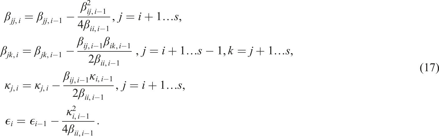
\begin{array}{c} β_{j j, i} = β_{j j, i - 1} - \frac{β_{i j, i - 1}^{2}}{4 β_{i i, i - 1}} & , j = i + 1 \dots s, \\ β_{j k, i} = β_{j k, i - 1} - \frac{β_{i j, i - 1} β_{i k, i - 1}}{2 β_{i i, i - 1}} & , j = i + 1 \dots s - 1, k = j + 1 \dots s, \\ κ_{j, i} = κ_{j, i} - \frac{β_{i j, i - 1} κ_{i, i - 1}}{2 β_{i i, i - 1}} & , j = i + 1 \dots s, \\ ϵ_{i} = ϵ_{i - 1} - \frac{κ_{i, i - 1}^{2}}{4 β_{i i, i - 1}} \end{array} .

(17)

The polynomial factors are derived analogously by

\begin{array}{c} b_{i} = \sqrt{\frac{π}{β_{i i, i - 1}}} b_{i - 1} - \frac{1}{2} \sqrt{\frac{π}{β_{i i, i - 1}^{3}}} (κ_{i, i - 1} c_{i, i - 1} - d_{i i, i - 1}) + \\ + \frac{1}{4} \sqrt{\frac{π}{β_{i i, i - 1}^{5}}} (κ_{i, i - 1}^{2} d_{i i, i - 1} - 3 κ_{i, i - 1} e_{i i i, i - 1}) - \frac{1}{8} \sqrt{\frac{π}{β_{i i, i - 1}^{7}}} κ_{i, i - 1}^{3} e_{i i i, i - 1}, \end{array}

(18)

\begin{array}{c} c_{j, i} = \sqrt{\frac{π}{β_{i i, i - 1}}} c_{j, i - 1} - \frac{1}{2} \sqrt{\frac{π}{β_{i i, i - 1}^{3}}} (κ_{i, i - 1} d_{i j, i - 1} + β_{i j, i - 1} c_{i, i - 1} - e_{i i j, i - 1}) + \\ + \frac{1}{4} \sqrt{\frac{π}{β_{i i, i - 1}^{5}}} (2 κ_{i, i - 1} β_{i j, i - 1} d_{i i, i - 1} + κ_{i, i - 1}^{2} e_{i i j, i - 1} - 3 β_{i j, i - 1} e_{i i i, i - 1}) - \\ - \frac{3}{8} \sqrt{\frac{π}{β_{i i, i - 1}^{7}}} κ_{i, i - 1}^{2} β_{i j, i - 1} e_{i i i, i - 1}, j = i + 1, \dots, s, \end{array}

(19)

\begin{array}{l} d_{j j, i} = \sqrt{\frac{π}{β_{i i, i - 1}}} d_{j j, i - 1} - \frac{1}{2} \sqrt{\frac{π}{β_{i i, i - 1}^{3}}} (β_{i j, i - 1} d_{i j, i - 1} + κ_{i, i - 1} e_{i j j, i - 1}) + \\ + \frac{1}{4} \sqrt{\frac{π}{β_{i i, i - 1}^{5}}} (β_{i j, i - 1}^{2} d_{i i, i - 1} + 2 β_{i j, i - 1} κ_{i, i - 1} e_{i i j, i - 1}) - \\ - \frac{3}{8} \sqrt{\frac{π}{β_{i i, i - 1}^{7}}} κ_{i, i - 1} β_{i j, i - 1}^{2} e_{i i i, i - 1}, j = i + 1, \dots, s, \end{array}

(20)

\begin{array}{c} d_{j k, i} = \sqrt{\frac{π}{β_{i i, i - 1}}} d_{j k, i - 1} \\ - \frac{1}{2} \sqrt{\frac{π}{β_{i i, i - 1}^{3}}} (β_{i j, i - 1} d_{i k, i - 1} + β_{i k, i - 1} d_{i j, i - 1} + κ_{i, i - 1} e_{i j k, i - 1}) + \\ + \frac{1}{2} \sqrt{\frac{π}{β_{i i, i - 1}^{5}}} (β_{i j, i - 1} β_{i k, i - 1} d_{i i, i - 1} + \\ + β_{i j, i - 1} κ_{i, i - 1} e_{i i k, i - 1} + β_{i k, i - 1} κ_{i, i - 1} e_{i i j, i - 1}) - \\ - \frac{3}{4} \sqrt{\frac{π}{β_{i i, i - 1}^{7}}} κ_{i, i - 1} β_{i j, i - 1}^{2} e_{i i i, i - 1}, j = i + 1 \dots s - 1, k = j + 1, \dots, s, \end{array}

(21)

\begin{array}{c} e_{j j j, i} = \sqrt{\frac{π}{β_{i i, i - 1}}} e_{j j j, i - 1} - \frac{1}{2} \sqrt{\frac{π}{β_{i i, i - 1}^{3}}} β_{i j, i - 1} e_{i j j, i - 1} + \\ + \frac{1}{4} \sqrt{\frac{π}{β_{i i, i - 1}^{5}}} β_{i j, i - 1}^{2} e_{i i j, i - 1} - \frac{1}{8} \sqrt{\frac{π}{β_{i i, i - 1}^{7}}} β_{i j, i - 1}^{3} e_{i i i, i - 1}, j = i + 1, \dots, s, \end{array}

(22)

\begin{array}{c} e_{j j k, i} = \sqrt{\frac{π}{β_{i i, i - 1}}} e_{j j k, i - 1} - \frac{1}{2} \sqrt{\frac{π}{β_{i i, i - 1}^{3}}} (β_{i k, i - 1} e_{i j j, i - 1} + β_{i j, i - 1} e_{i j k, i - 1}) + \\ + \frac{1}{4} \sqrt{\frac{π}{β_{i i, i - 1}^{5}}} (β_{i j, i - 1}^{2} e_{i i k, i - 1} + 2 β_{i j, i - 1} β_{i k, i - 1} e_{i i j, i - 1}) - \\ - \frac{3}{8} \sqrt{\frac{π}{β_{i i, i - 1}^{7}}} β_{i j, i - 1}^{2} β_{i k, i - 1} e_{i i i, i - 1}, j = i + 1 \dots s - 1, k = j + 1, \dots, s, \end{array}

(23)

\begin{array}{c} e_{j k k, i} = \sqrt{\frac{π}{β_{i i, i - 1}}} e_{j k k, i - 1} - \frac{1}{2} \sqrt{\frac{π}{β_{i i, i - 1}^{3}}} (β_{i j, i - 1} e_{i k k, i - 1} + β_{i k, i - 1} e_{i j k, i - 1}) + \\ + \frac{1}{4} \sqrt{\frac{π}{β_{i i, i - 1}^{5}}} (β_{i k, i - 1}^{2} e_{i i j, i - 1} + 2 β_{i j, i - 1} β_{i k, i - 1} e_{i i k, i - 1}) - \\ - \frac{3}{8} \sqrt{\frac{π}{β_{i i, i - 1}^{7}}} β_{i j, i - 1} β_{i k, i - 1}^{2} e_{i i i, i - 1}, j = i + 1 \dots s - 1, k = j + 1, \dots, s, \end{array}

(24)

\begin{array}{c} e_{j k l, i} = \sqrt{\frac{π}{β_{i i, i - 1}}} e_{j k l, i - 1} - \\ - \frac{1}{2} \sqrt{\frac{π}{β_{i i, i - 1}^{3}}} (β_{i j, i - 1} e_{i k l, i - 1} + β_{i k, i - 1} e_{i j l, i - 1} + β_{i l, i - 1} e_{i j k, i - 1}) + \\ + \frac{1}{2} \sqrt{\frac{π}{β_{i i, i - 1}^{5}}} (β_{i j, i - 1} β_{i k, i - 1} e_{i i l, i - 1} + \\ + β_{i j, i - 1} β_{i l, i - 1} e_{i i k, i - 1} + β_{i k, i - 1} β_{i l, i - 1} e_{i i j, i - 1}) - \\ - \frac{3}{4} \sqrt{\frac{π}{β_{i i, i - 1}^{7}}} β_{i j, i - 1} β_{i k, i - 1} β_{i l, i - 1} e_{i i i, i - 1};, \\ j = i + 1, \dots, s - 2, k = j + 1, \dots, s - 1, l = k + 1, \dots, s \end{array}

(25)

The last integration step s includes the sgn() function. Therefore, the results need to be calculated differently, but can still be derived analytically:

\begin{array}{c} I_{1,2} = \frac{1}{\sqrt{{(2 π)}^{s} | V |}} \\ (- \sqrt{\frac{π}{β_{s s, s - 1}}} b_{s - 1} + \frac{1}{2} \sqrt{\frac{π}{β_{s s, s - 1}^{3}}} κ_{s, s - 1} c_{s, s - 1} - \\ - \frac{1}{4} \sqrt{\frac{π}{β_{s s, s - 1}^{5}}} (κ_{s, s - 1}^{2} + 2 β_{s s, s - 1}) d_{s s, s - 1} + \\ + \frac{1}{8} \sqrt{\frac{π}{β_{s s, s - 1}^{7}}} (κ_{s, s - 1}^{3} + 6 β_{s s, s - 1} κ_{s, s - 1}) e_{s s s, s - 1}) \cdot \\ \cdot \erf (\frac{κ_{s, s - 1}}{2 \sqrt{β_{s s, s - 1}}}) e^{\frac{κ_{s, s - 1}^{2}}{4 β_{s s, s - 1}} - ϵ_{s - 1}} + \\ + (\frac{1}{β_{s s, s - 1}} c_{s, s - 1} - \frac{κ_{s, s - 1}}{2 β_{s s, s - 1}^{2}} d_{s s, s - 1} + \\ + \frac{κ_{s, s - 1}^{2} + 4 β_{s s, s - 1}}{4 β_{s s, s - 1}^{3}} e_{s s s, s - 1}) \cdot e^{- ϵ_{s - 1}} . \end{array}

(26)

The erf() function does not allow further analytical integrations. Therefore, the integration with respect to the sgn() function is done as the last step.

The existence and the uniqueness of the stationary response for the case α_t > 0 was proven¹. For the case α_t = 0, no stationary case exists. The accuracy of the second order equation can be taken from the Fokker–Planck–Kolmogorov equation because the used equations are using the moments of the Fokker–Planck–Kolmogorov equation. Although the moments are derived from the Fokker–Planck–Kolmogorov equations and are accurate, the closure technique needed to reduce higher moments is only accurate as long as the distribution is of Gaussian type. Therefore, if the distribution is non-Gaussian, the results for the first and second order moments are only approximations of the real values. For non-linear behavior, the distributions of the resulting variables are non-Gaussian, even if the load is of Gaussian type. Especially, the distribution of the stress proportional displacement z is limited to the range from −1 to 1 for softening behavior and cannot be reproduced by a Gaussian distribution. This becomes important for high values of plasticity which are investigated here to find the limitations of the approach. An unevenness introduced by the force proportional displacement z₀ also increases the deviations from the real values.

The accuracy of the approximation by a discrete time step procedure is only checked in the adaptive implicit Radau method. The absolute and the relative error are both limited to 10⁻⁶. It is not checked by the simple time step procedure and the Runge–Kutta RK4 method. To have stability, a very short time step of 10⁻⁶ is needed. So the inaccuracy of the numerical iteration should be negligible.

Results for a tank under filtered white noise excitation

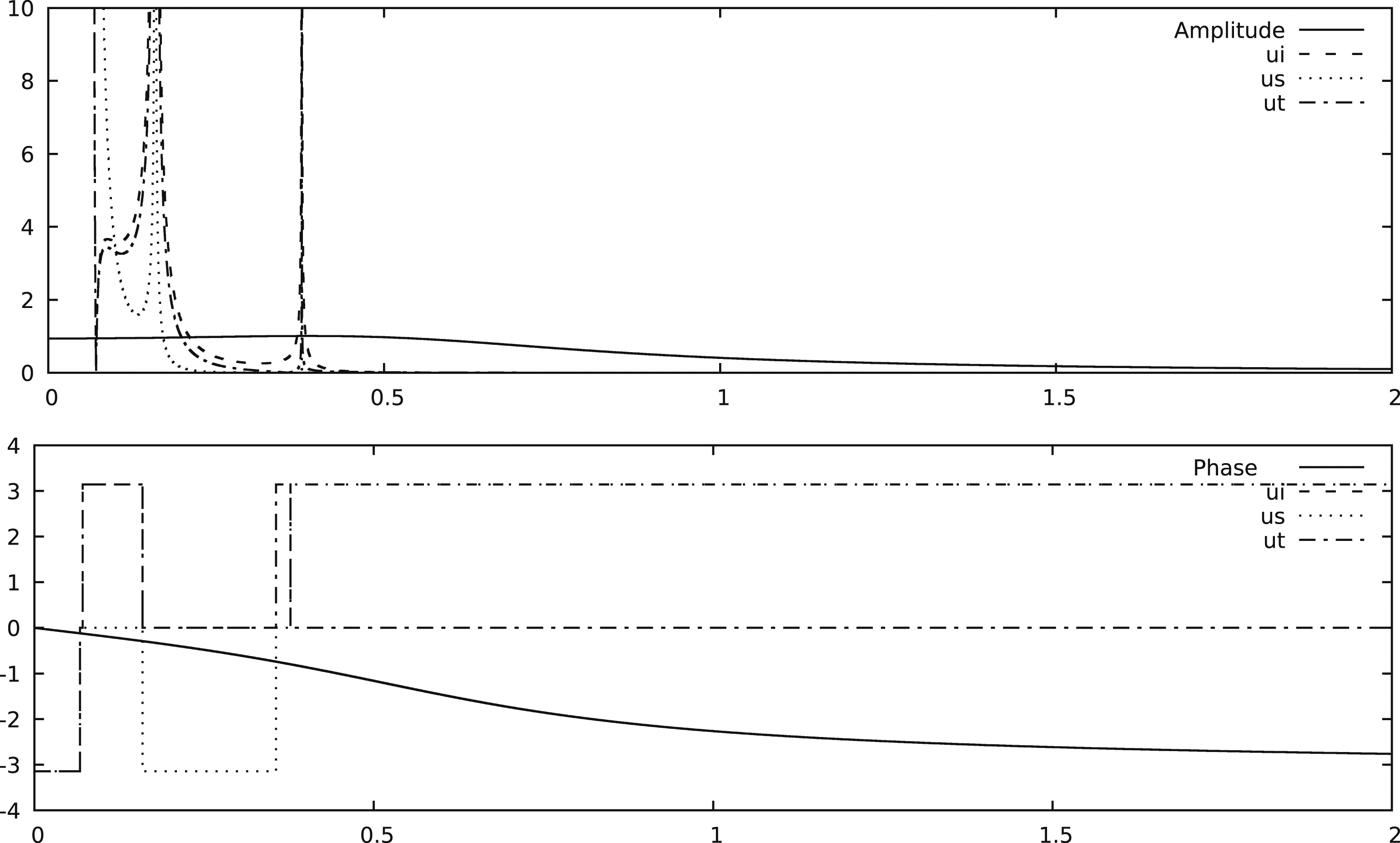
The filter has the following parameters: m_f = 0.06667, c_f = 0.3, k_f = 1.06667, and K_f = 0.5. The amplitude and the phase of the filter are presented in Figure 2. The displacement of the filter is named x_f and its derivative v_f. Physically the displacement acts as an acceleration and the velocity as a jerk. In Figure 2, the spectrum of the tank for the linear system with an linear spring instead of the hysteretic element is presented. The transfer functions of the system for the tank (u_t), the impulsive mass (u_i), and the sloshing mass (u_s) are added in Figure 2. The high resonance frequency is caused by the impulsive mass that is coupled with the tank using a stiff spring.

Figure 2.

Filter spectrum with amplitude and phase as ordinate and normalized frequency as abscissa. Additionally, the transfer function between ground acceleration and absolute displacements of the fully elastic model (α_t = 1.0) are presented for the impulsive mass (u_i), the sloshing mass (u_s), and the tank (u_t).

The examples are made in dimensionless coordinates and the elastic-plastic limit of the stresses is given by the interval from minus one to one.

For the tank mass, the parameters m_t = 1.0, c_t = 0.0, k_t = 1.0, and α_t = 0.0 are used. The Bouc hysteresis is parametrized by A = 1.0, γ = 0.5, and θ = 0.5 and the eccentricity of the hysteresis loop is given by z₀ = 0.5. The sloshing mass has the parameters m_s = 0.5, c_s = 0.0, and k_s = 0.1. The impulsive mass is coupled more stiffly with m_i = 0.1, c_i = 0.0, and k_i = 0.5.

The Monte Carlo method uses the same time step procedures for every realization of the process. 100,000 realizations were processed because time averaging is not possible in the transient case.

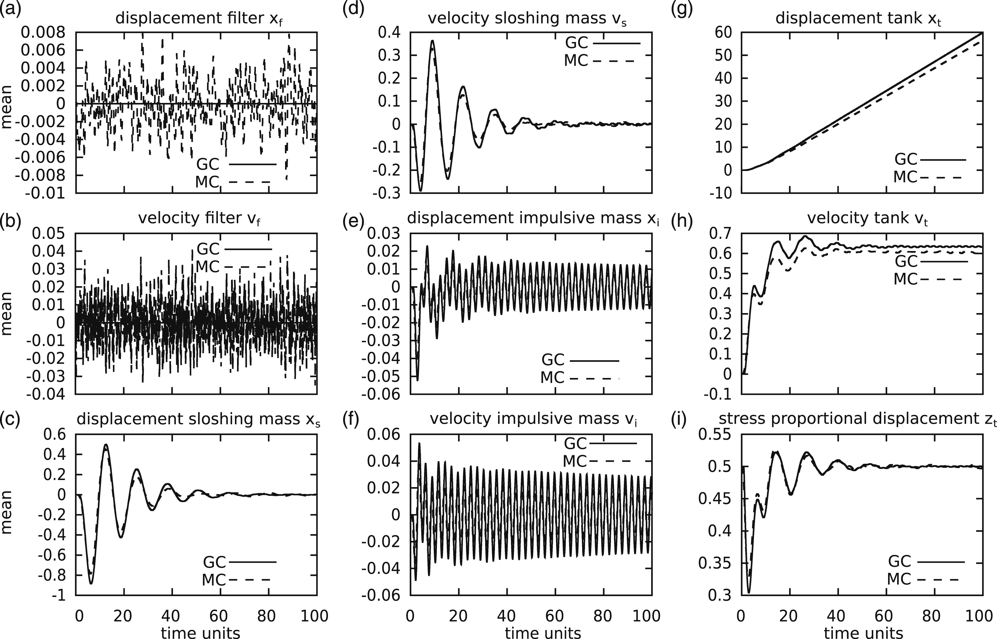
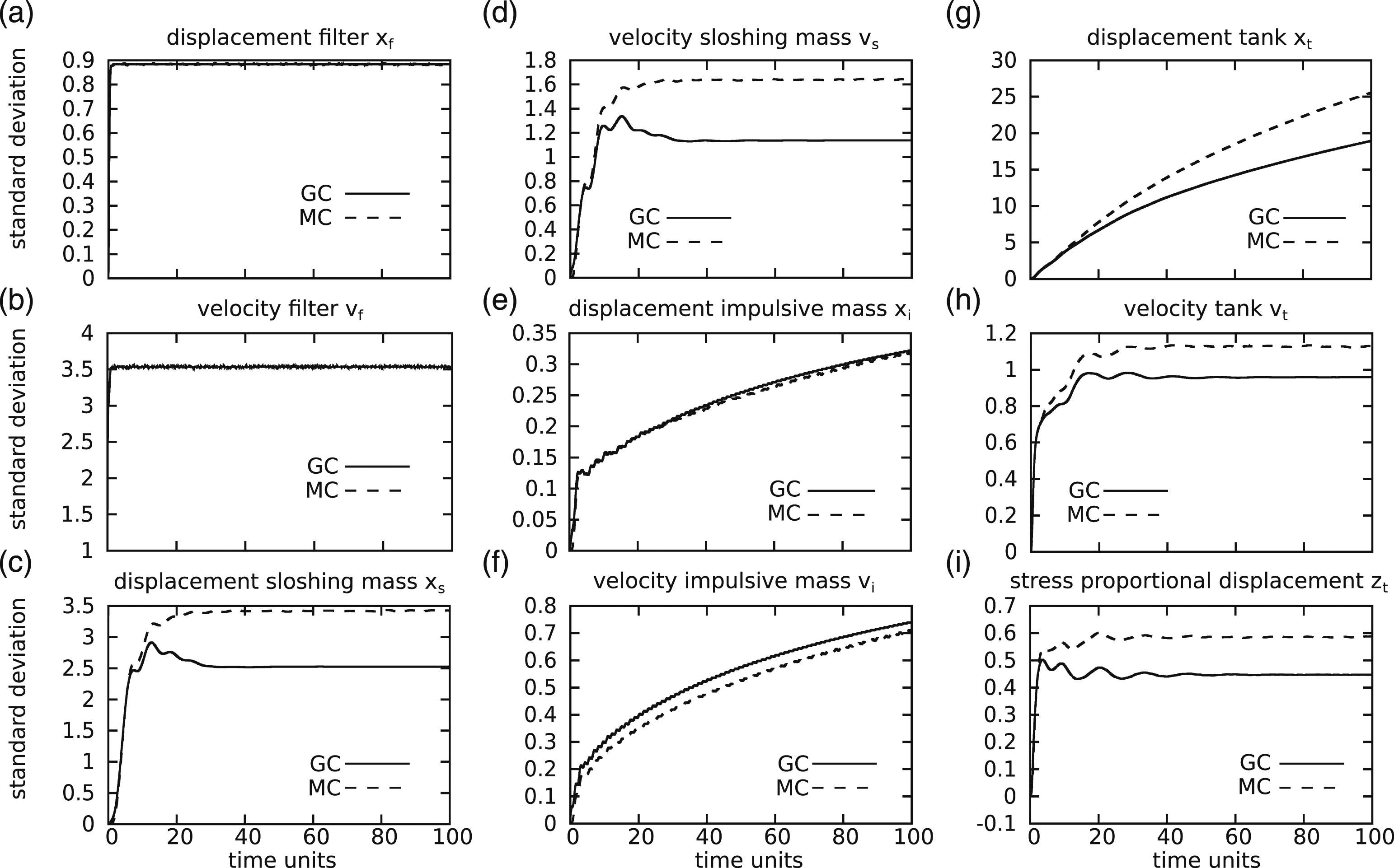
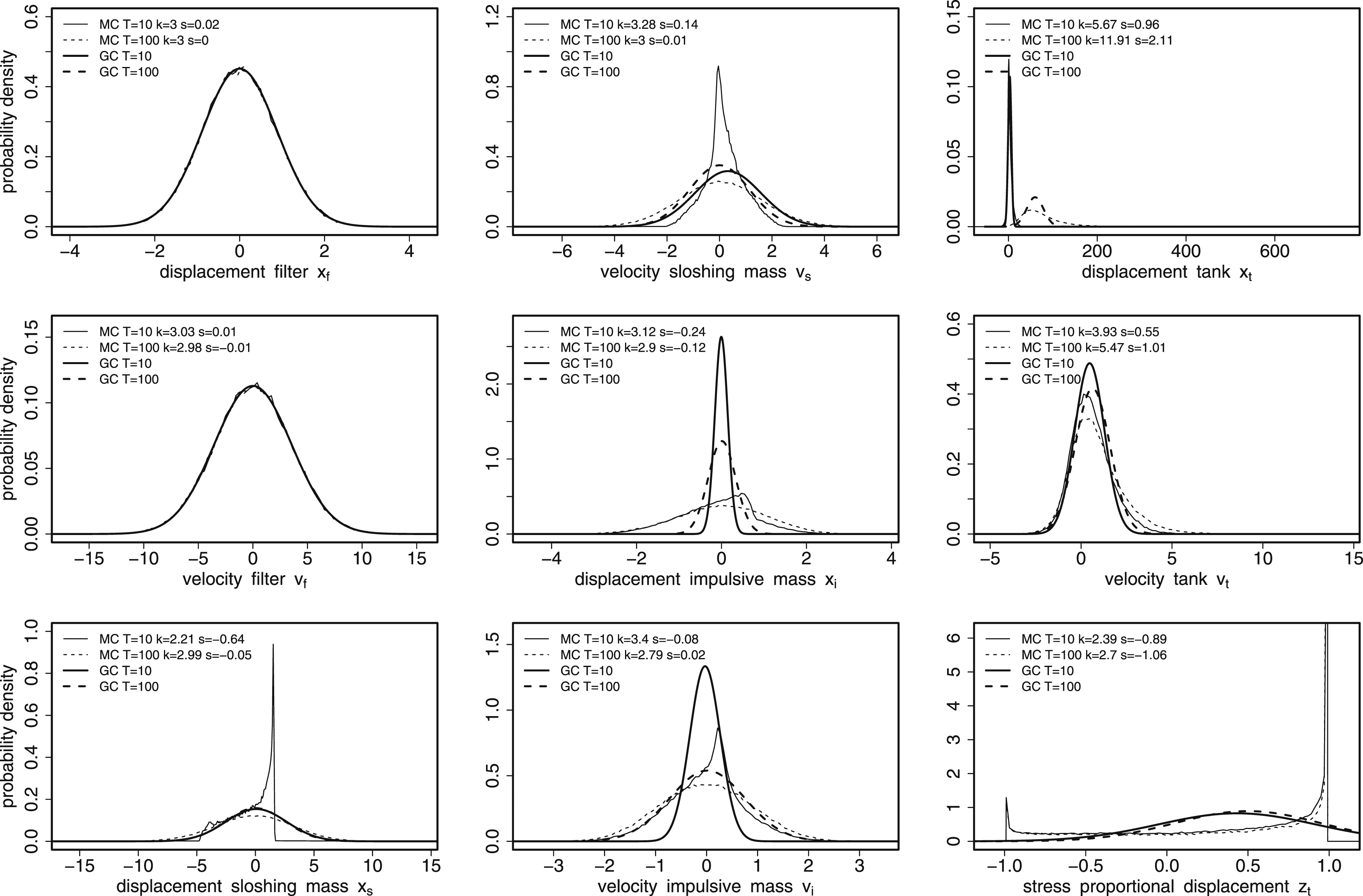
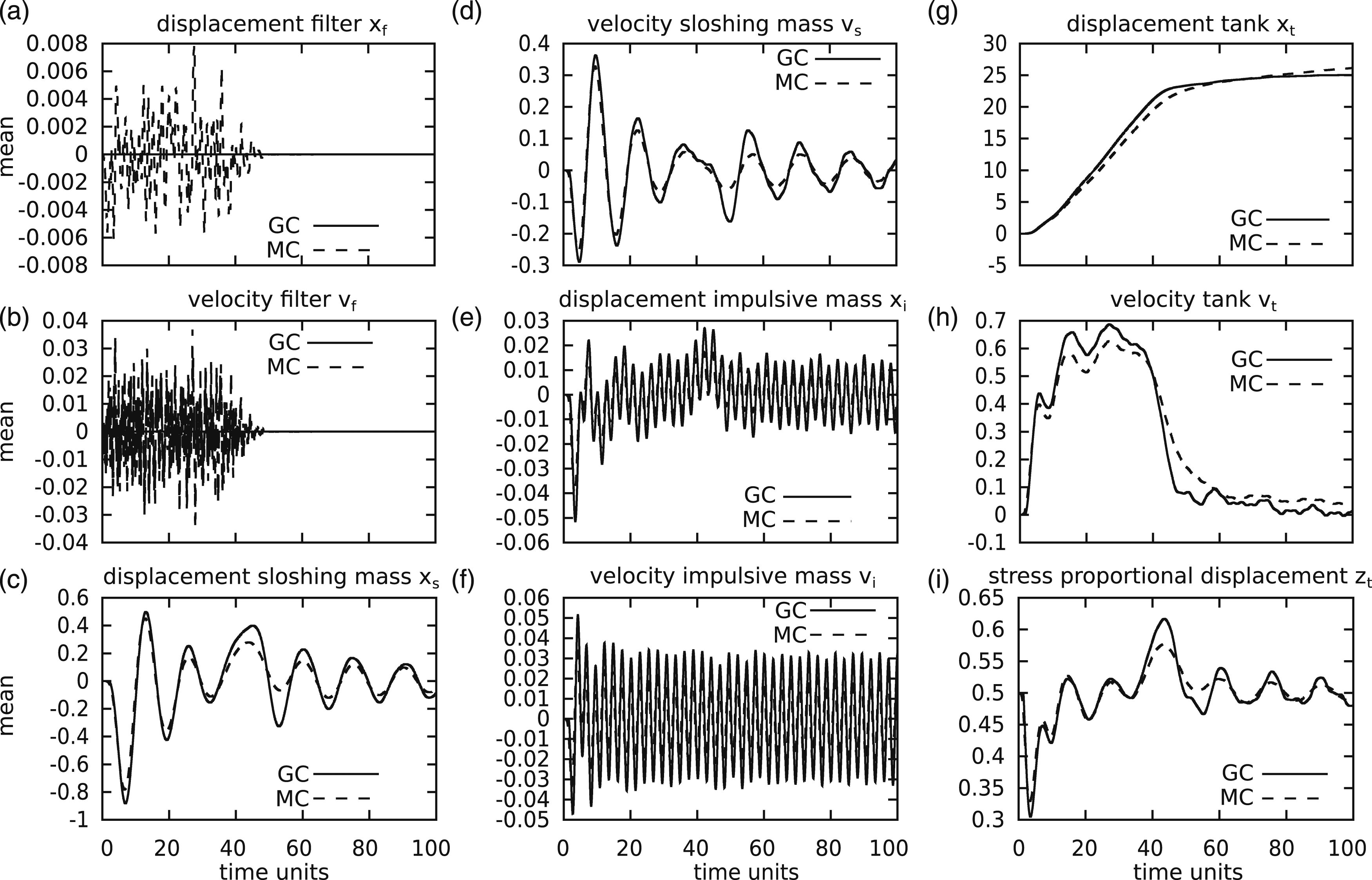
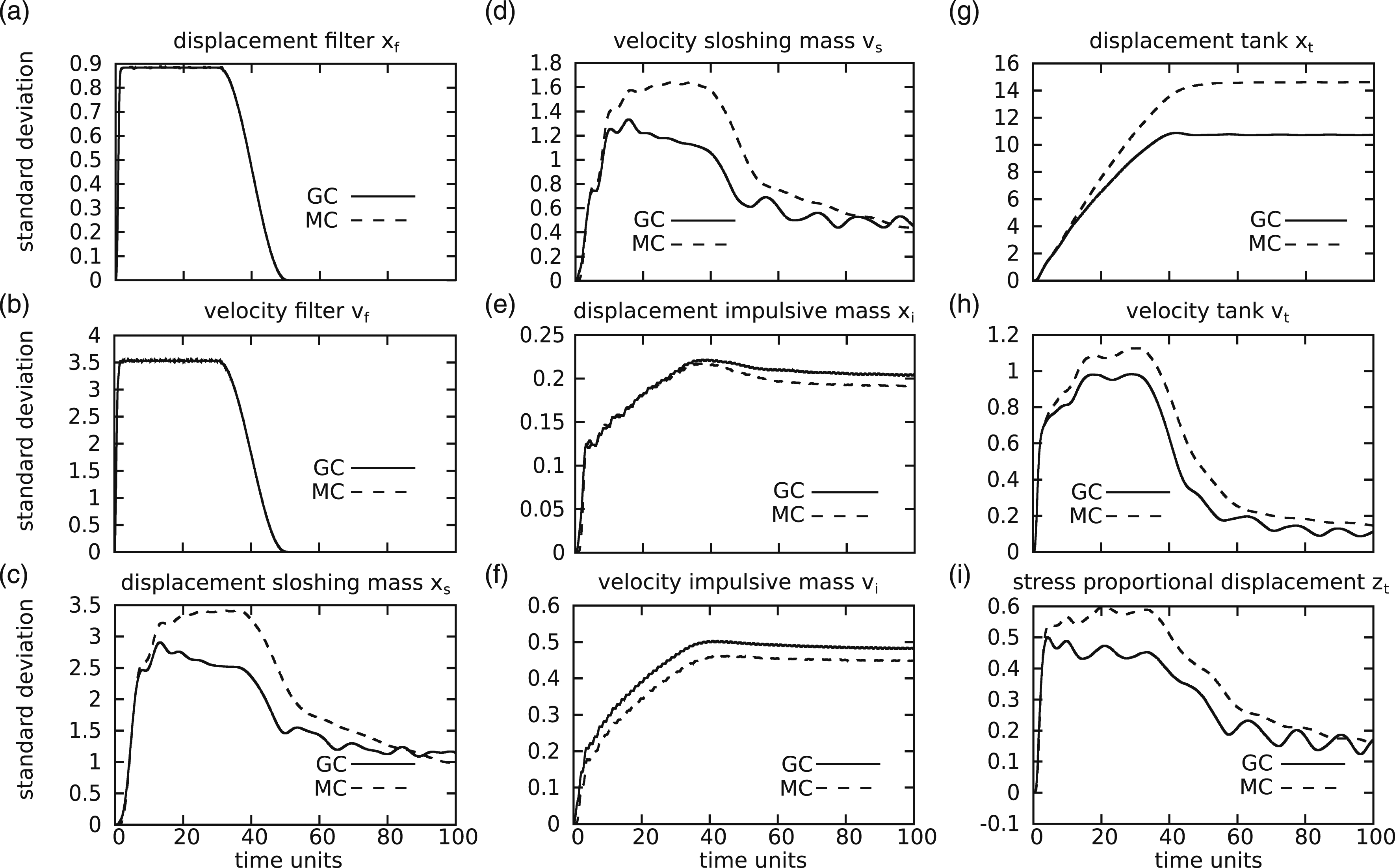
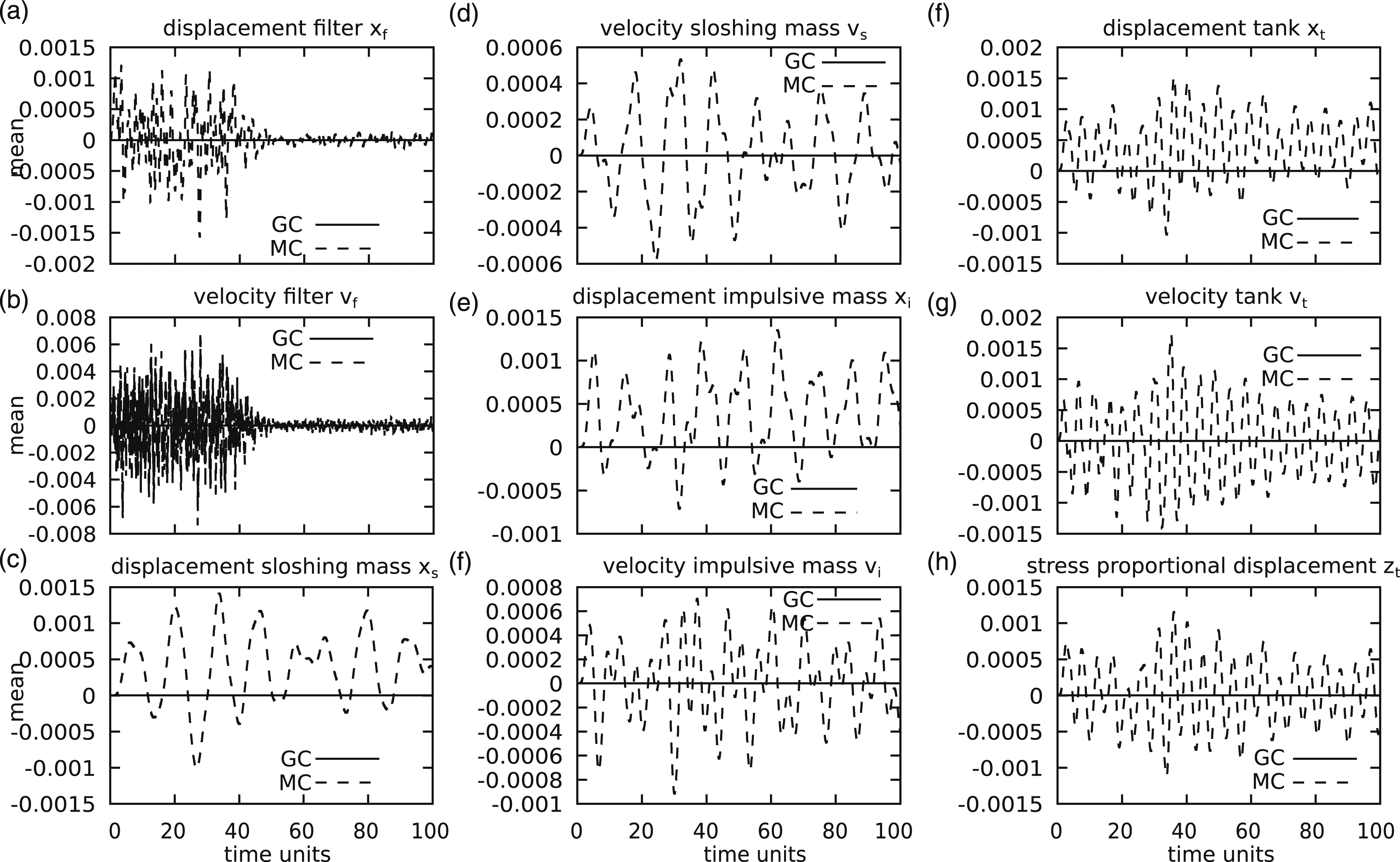
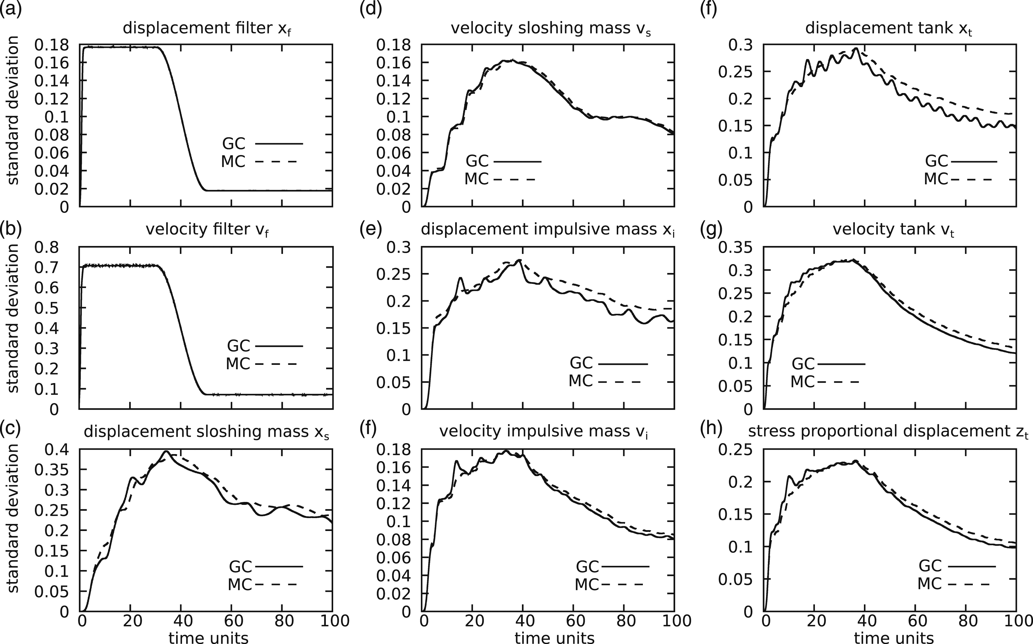
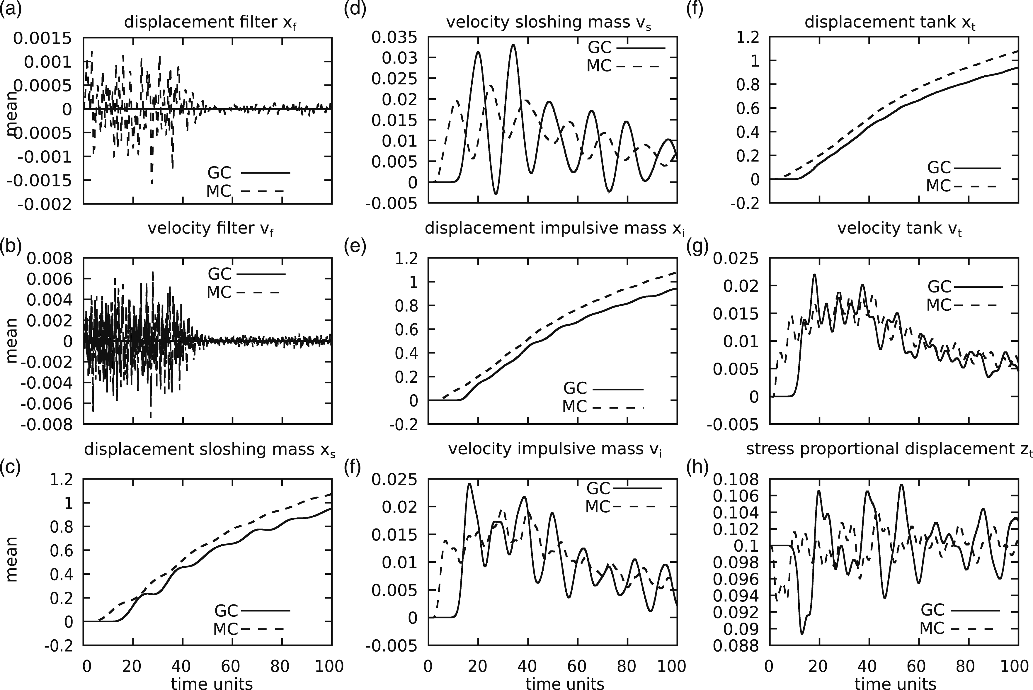
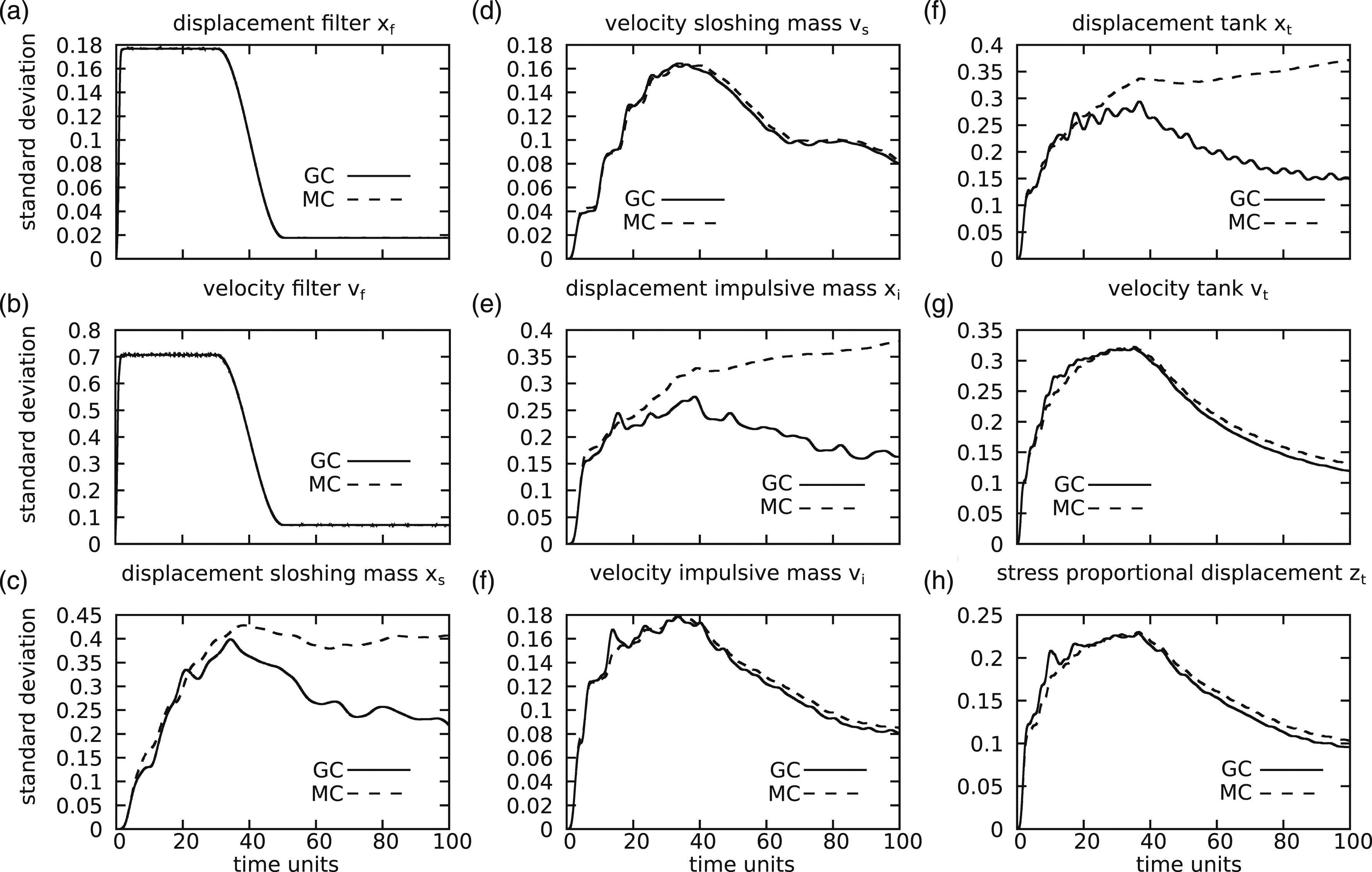
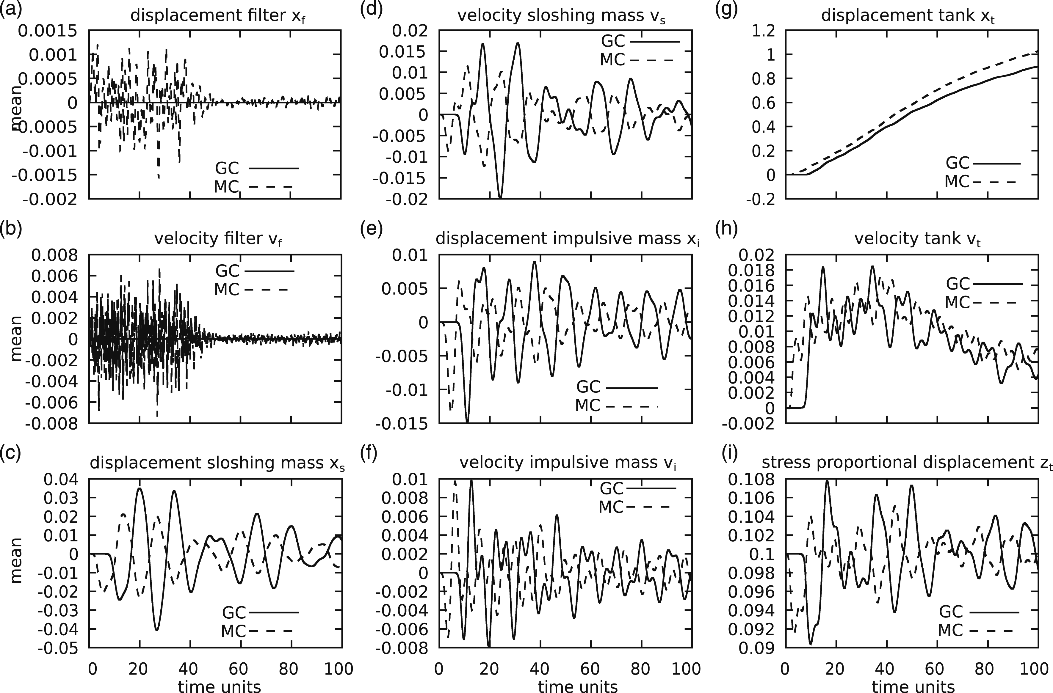
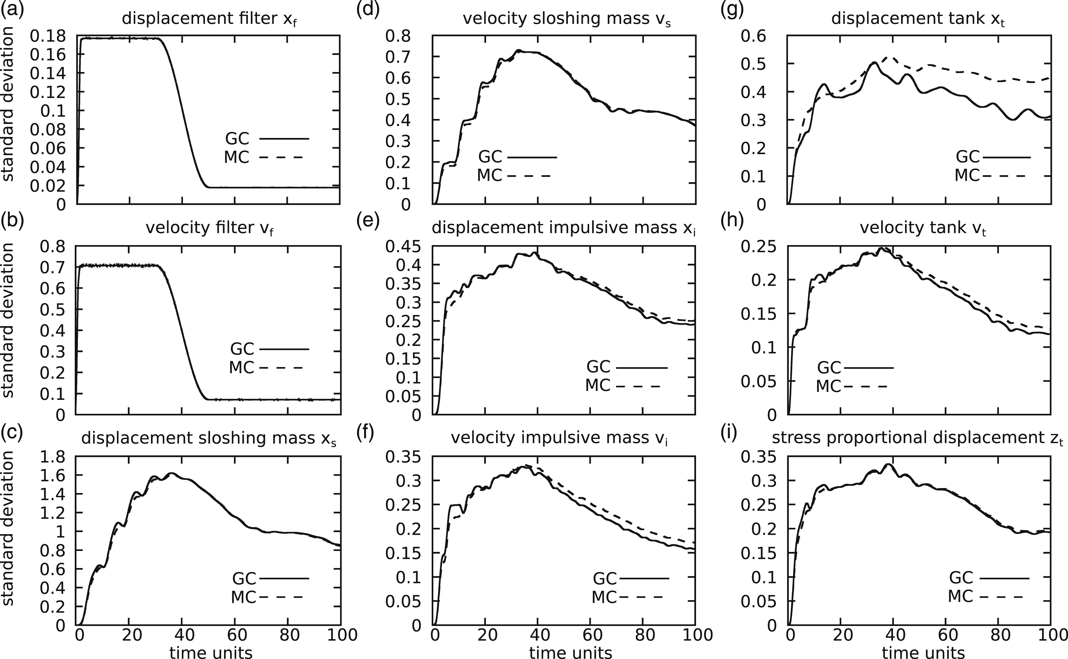
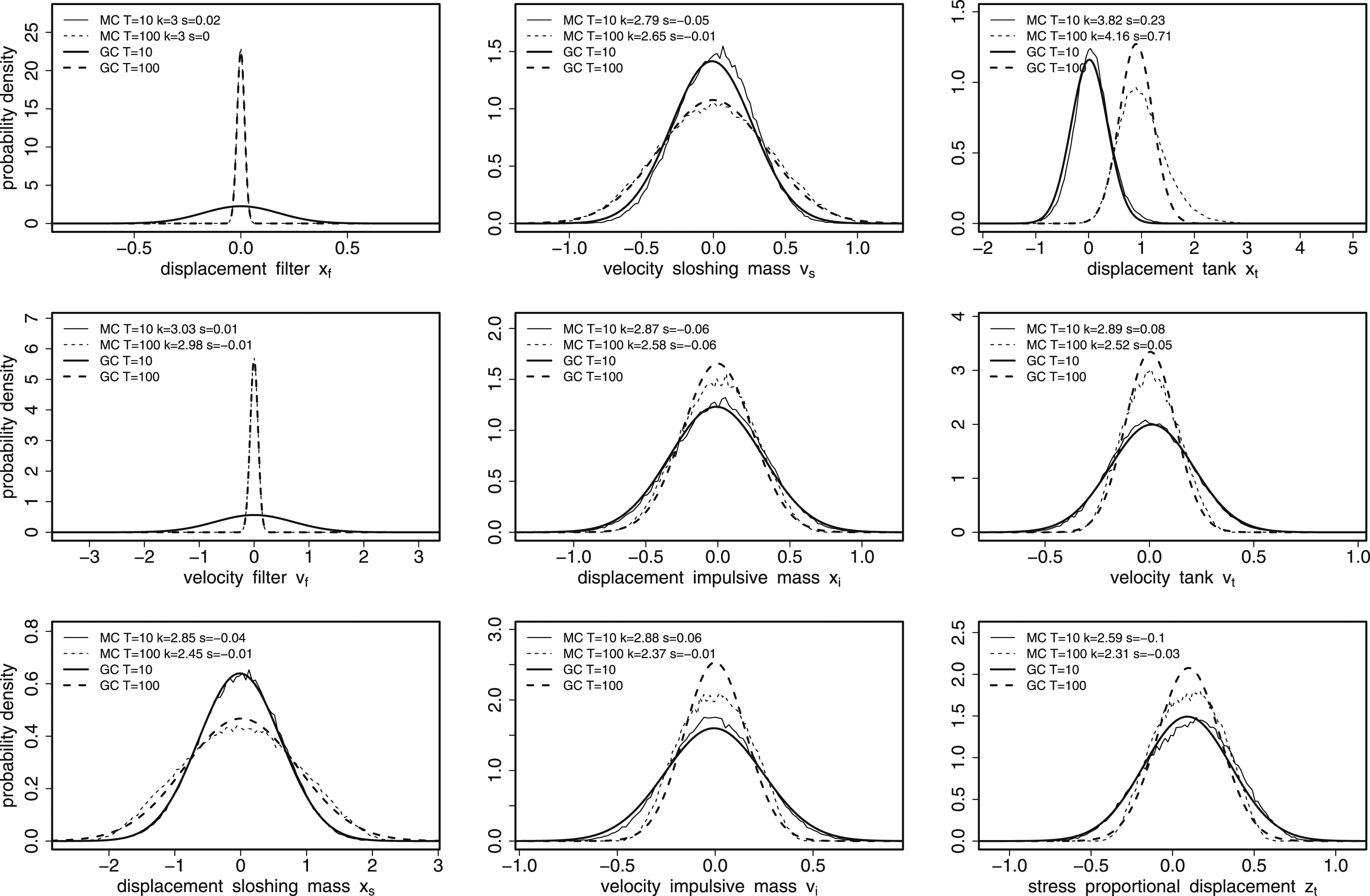
In Figure 3, the absolute displacements for the tank, the sloshing, and the impulsive mass are presented. The results for the moments from the Gaussian closure technique show some deviations from to the results from the Monte Carlo simulation. It becomes visible that the displacement of the tank dominates in Figure 3 because the absolute displacements of the DOFs behave similar. This can become a problem, as the relative displacements between the masses are very small and therefore the coherence is very high and a coherent behavior cannot be handled by the used integrator thus far. The described stabilization measures help to avoid division by zero errors and a singular matrix. In Figure 4, the mean values are reproduced and in Figure 5, the standard deviation of all state vector variables is reproduced. The filter output is reproduced exactly because the filter is itself linear and only acts as an input to the non-linear system with no feedback. While the mean values of the structure are reproduced almost exactly, the standard deviations show some differences that are caused by the high level of excitation with respect to the elasto-plastic limit of the Bouc hysteresis. In Figure 6, it can be seen clearly that for a very high loading K₀ and a large z₀ with respect to the plastic limits some quantities exhibit large deviations of the distributions derived using the Monte Carlo method from the Gaussian assumption. While the distribution of the force proportional displacement z_t is somehow correctly estimated, the velocities and displacements are completely different. This has to do with the limits of the z_t-distribution to the interval [−1, 1], whereas the assumed Gaussian distribution extends from [ −∞, ∞]. So the distribution contains values that are physically not defined. These limits are clearly reached in the z_t-distribution and lead to high peaks in the displacements and velocities of the remaining variables x_s, v_s, x_t, v_t, x_i, v_i. For the tank x_t, the shift of the mean is not reproduced by the Gaussian closure technique. Also, the covariances are based on the assumption of a multivariate Gaussian distribution and couple the displacements and the velocities in an non-exact manner. Therefore, also the standard deviation of the remaining variables of the tank is underestimated in most cases. The standard deviations of the displacement and velocity of the impulsive mass are slightly overestimated. In the following examples, more realistic lower amplitudes of the loading shall be investigated. A possible method to improve the situation could be to fit the two moments to a beta-distribution, if the distribution or higher moments are needed.³⁷

Figure 3.

Stationary colored noise (K_t = 0.5, z₀ = 0.5): Absolute displacements of the tank (t), the impulsive mass (i), and the sloshing mass (s). Presented are the mean values (M) and the mean values ± standard deviation (M ± S) for the Gaussian closure method (GC) and the Monte Carlo simulation (MC).

Figure 4.

Stationary colored noise (K_t = 0.5, z₀ = 0.5): Mean values of displacement (x), velocities (v), and stress proportional displacements (z) of the filter (f), the tank (t), the impulsive mass (i), and the sloshing mass (s) for the Gaussian closure method (GC) and the Monte Carlo simulation (MC).

Figure 5.

Stationary colored noise (K_t = 0.5, z₀ = 0.5): Standard deviations of displacement (x), velocities (v), and stress proportional displacements (z) of the filter (f), the tank (t), the impulsive mass (i), and the sloshing mass (s) for the Gaussian closure method (GC) and the Monte Carlo simulation (MC).

Figure 6.

Absolute DOFs with (K_t = 0.5, z₀ = 0.5): Histogram of displacement (x), velocities (v), and stress proportional displacements (z) of the filter (f), the tank (t), the impulsive mass (i), and the sloshing mass (s) for the Gaussian closure method (GC) and the Monte Carlo simulation (MC) at 10 and 100 time units. Kurtosis (k) and skewness (s) are given for the Monte Carlo results. The Gaussian distributions have a kurtosis of 3 and a skewness of 0.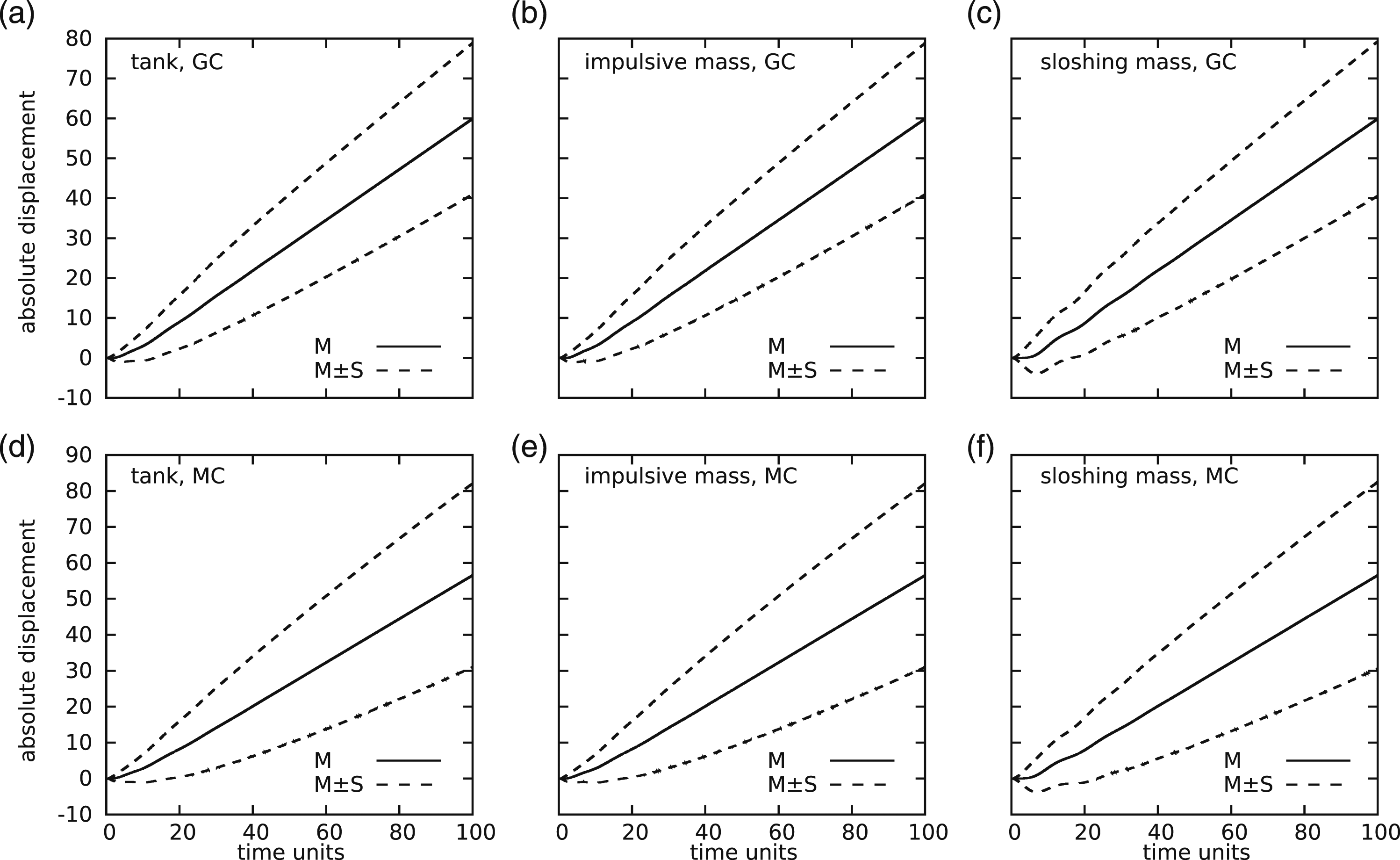

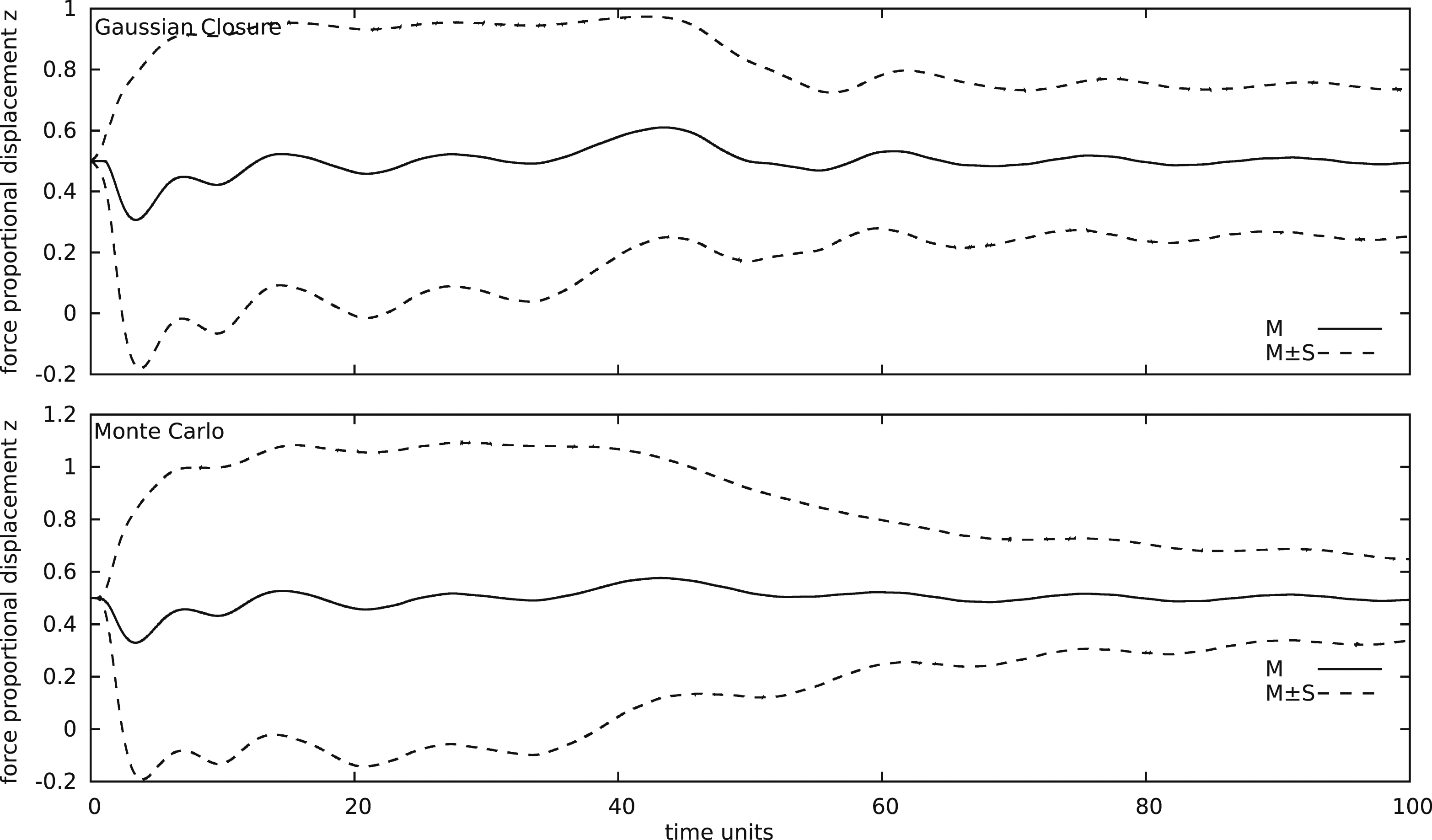
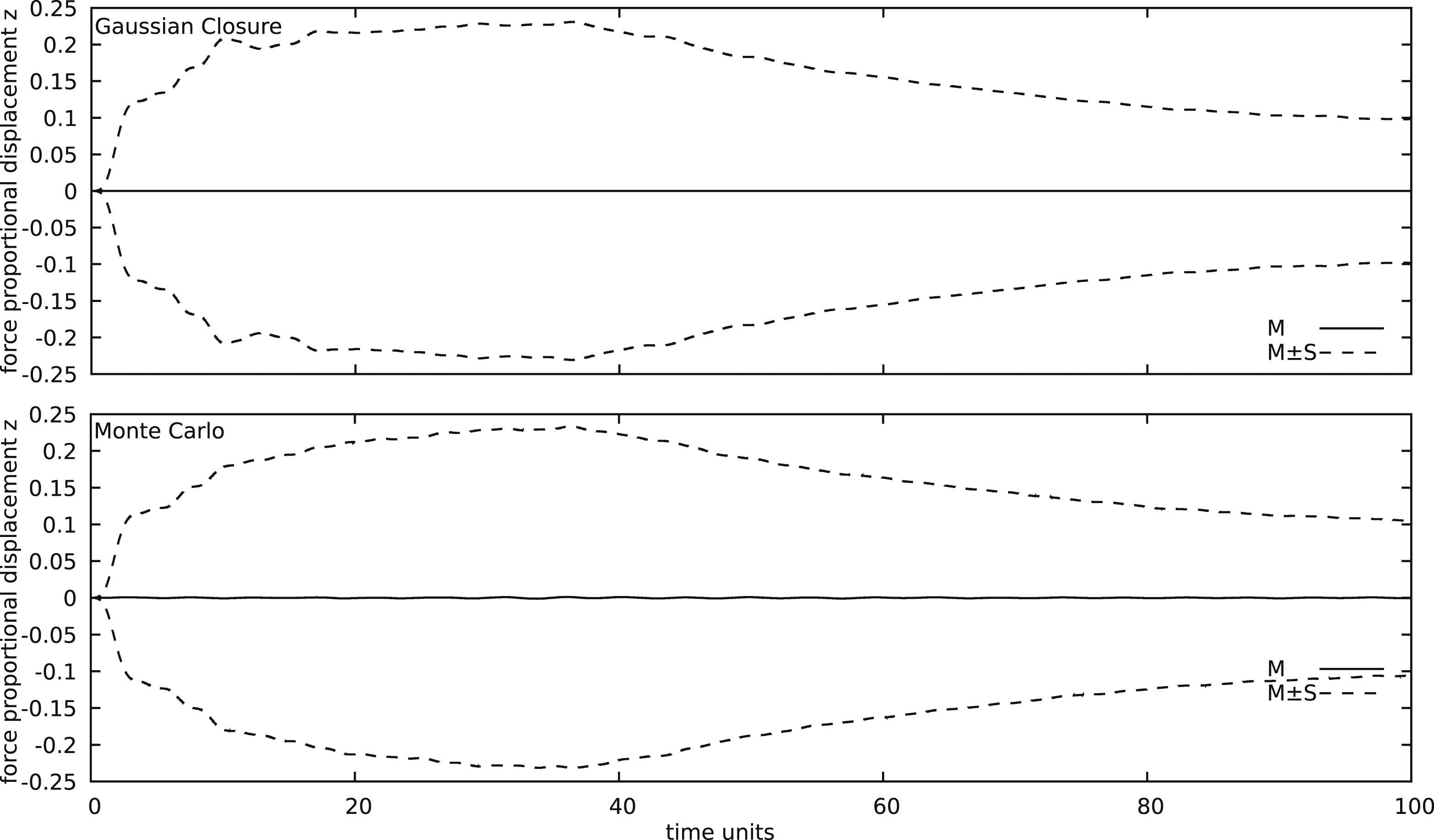
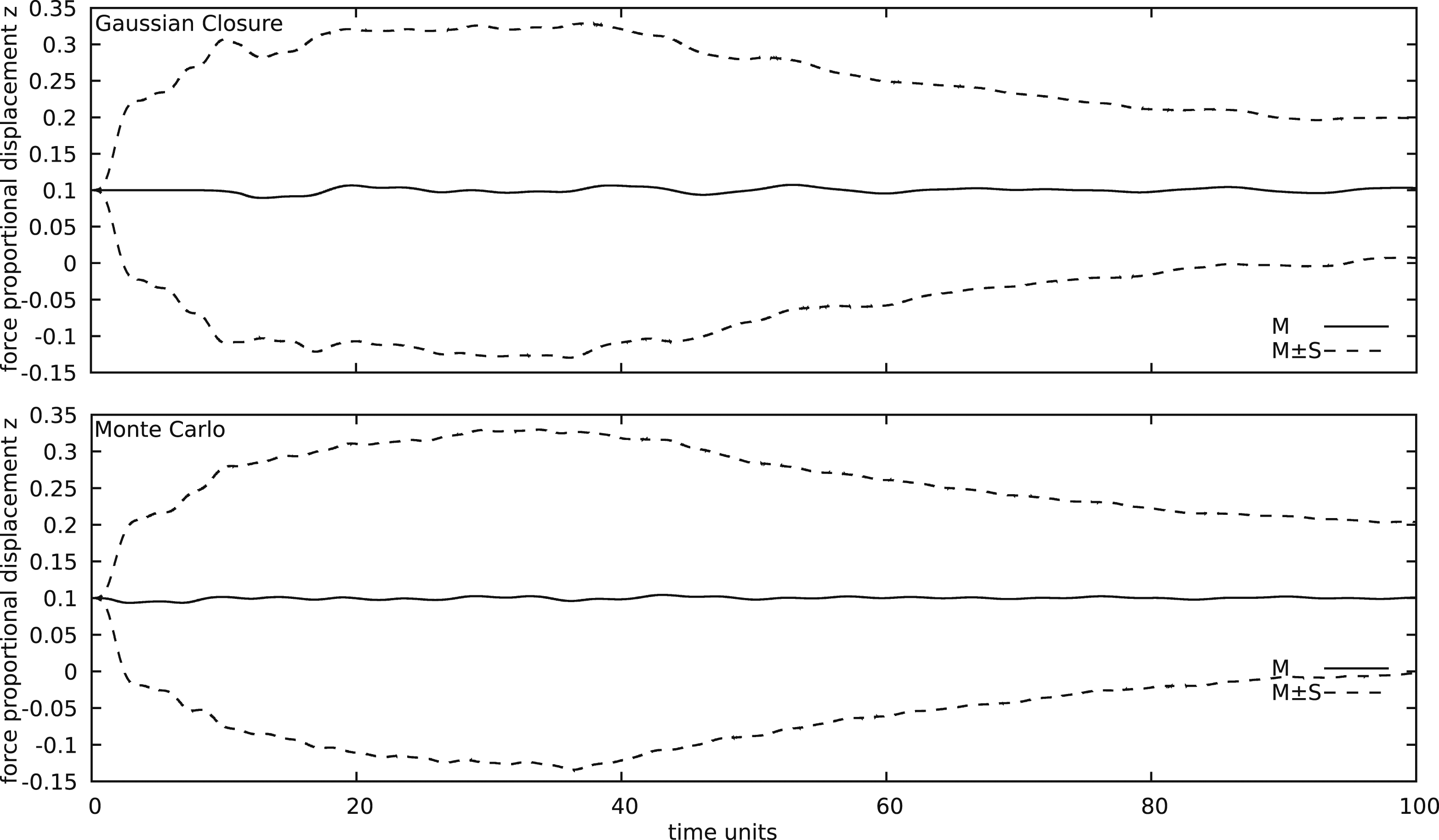
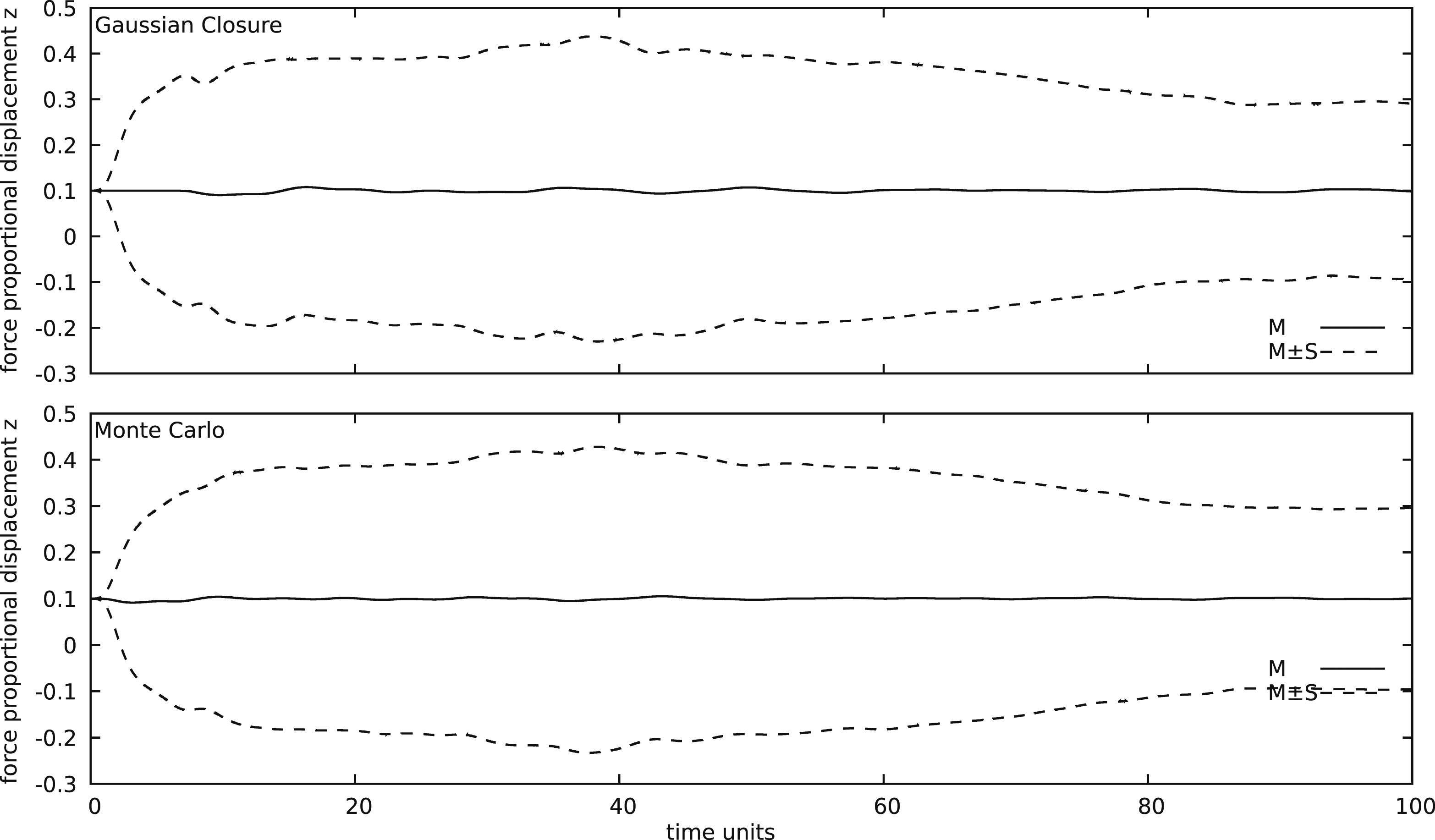
In Figure 7, the mean values and the standard deviation of z_t are presented. It becomes clear that the upper limit lies in the region of mean value plus standard deviation. It is also visible that the Gaussian closure technique still coincides with the result of the Monte Carlo simulation.

Figure 7.

Stationary colored noise (K_t = 0.5, z₀ = 0.5): Force proportional displacement z_t. Presented are the mean values (M) and the mean values ± standard deviation (M ± S) for the Gaussian closure method (GC) and the Monte Carlo simulation (MC).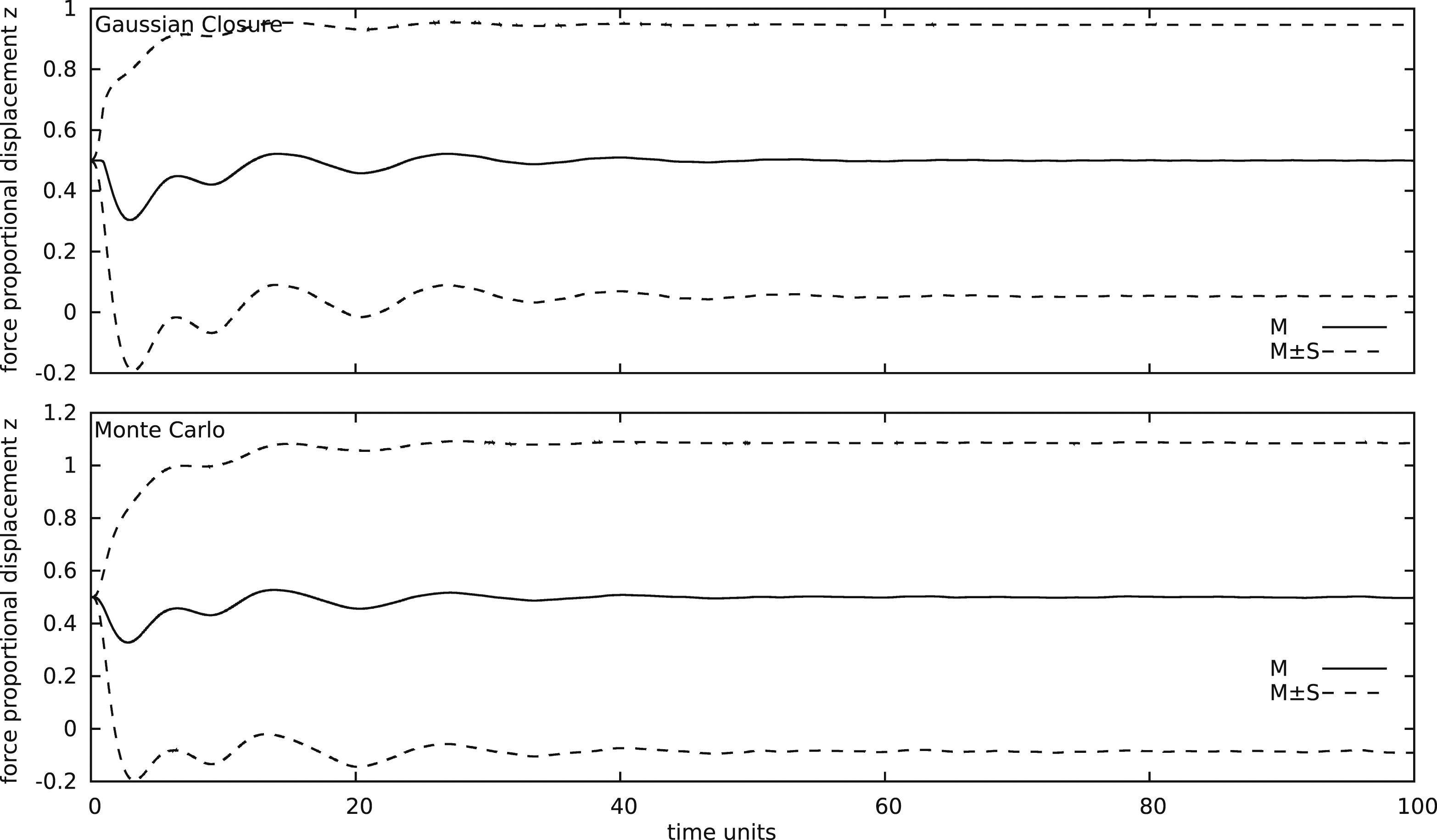

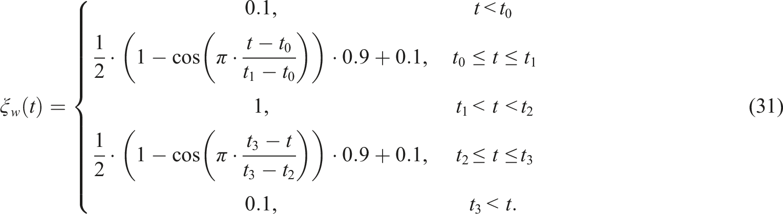
In a second example, the intensity of the white excitation used as input to the filter is made time dependent²³ (equation (27)). A tapered window was used (equation (28)):

\begin{array}{l} ξ_{f} (t) = ξ_{0} (t) \cdot ξ_{w} (t) \\ K_{f} (t) = K_{0} \cdot ξ_{w} {(t)}^{2} \end{array}

(27)

ξ_{w} (t) = {\begin{array}{c} 0, & t < t_{0} \\ \frac{1}{2} \cdot (1 - \cos (π \cdot \frac{t - t_{0}}{t_{1} - t_{0}})), & t_{0} \leq t \leq t_{1} \\ 1, & t_{1} < t < t_{2} \\ \frac{1}{2} \cdot (1 - \cos (π \cdot \frac{t_{3} - t}{t_{3} - t_{2}})), & t_{2} \leq t \leq t_{3} \\ 0, & t_{3} < t . \end{array}

(28)

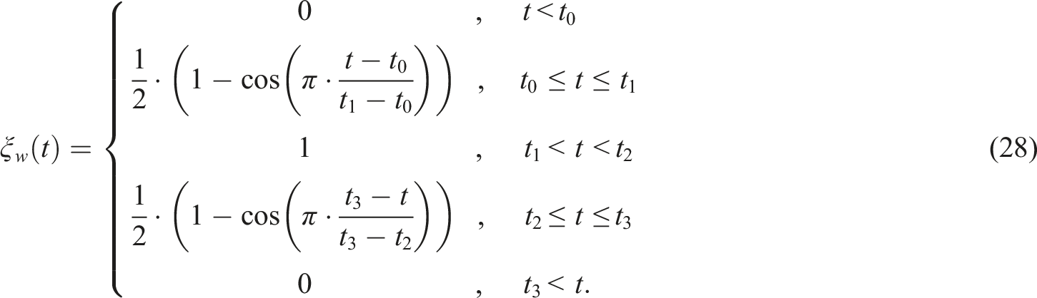
The parameters of the window are set to t₀ = 0.0, t₁ = 1.0, t₂ = 30.0, and t₃ = 50.0 (Figure 8).

Figure 8.

Window function and squared window function with respect to normalized time.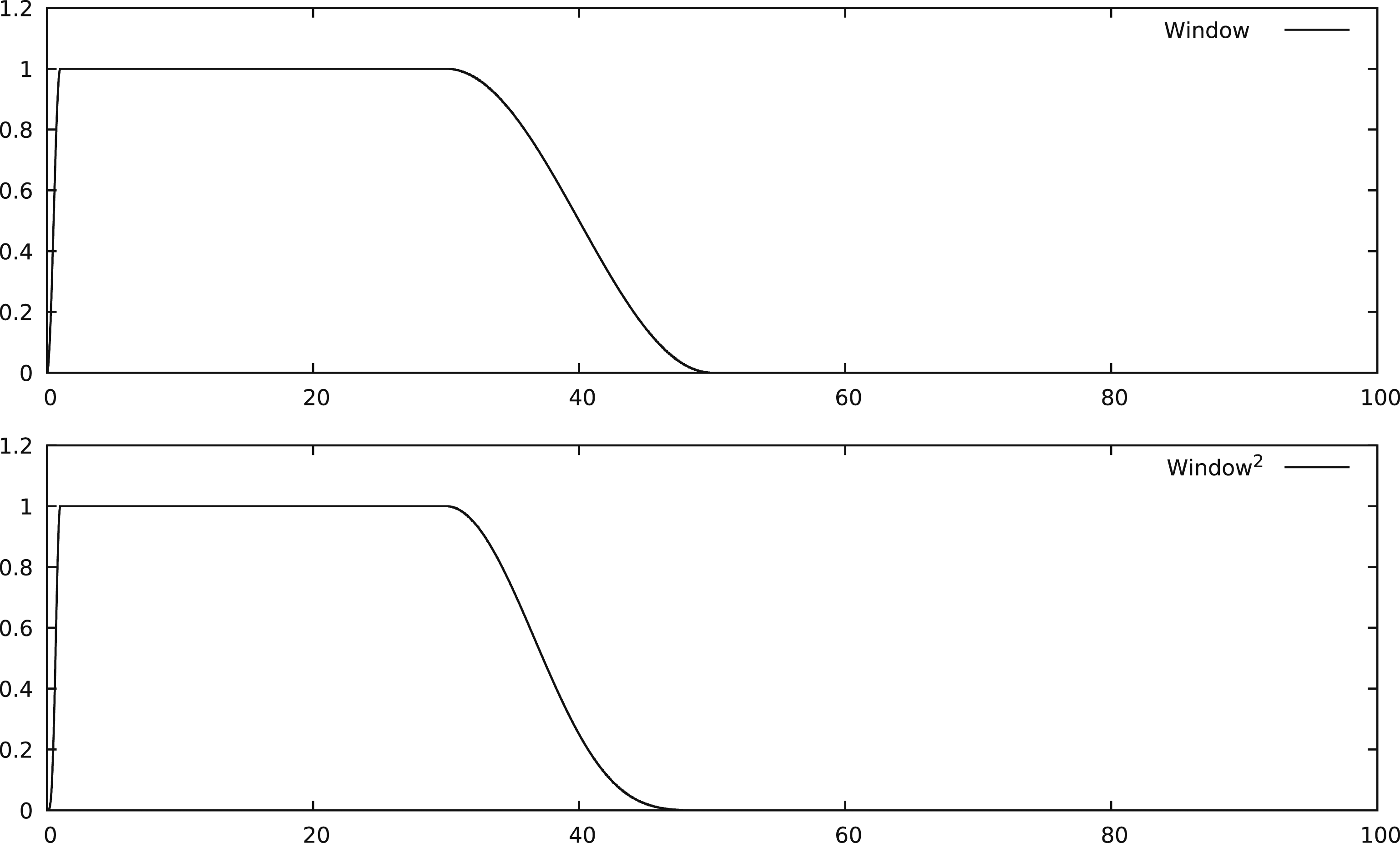

The magnitude of the white noise process is set to K₀ = 0.5 in accordance with K_f = 0.5 in the first example. All remaining parameters are unchanged with respect to the first example.

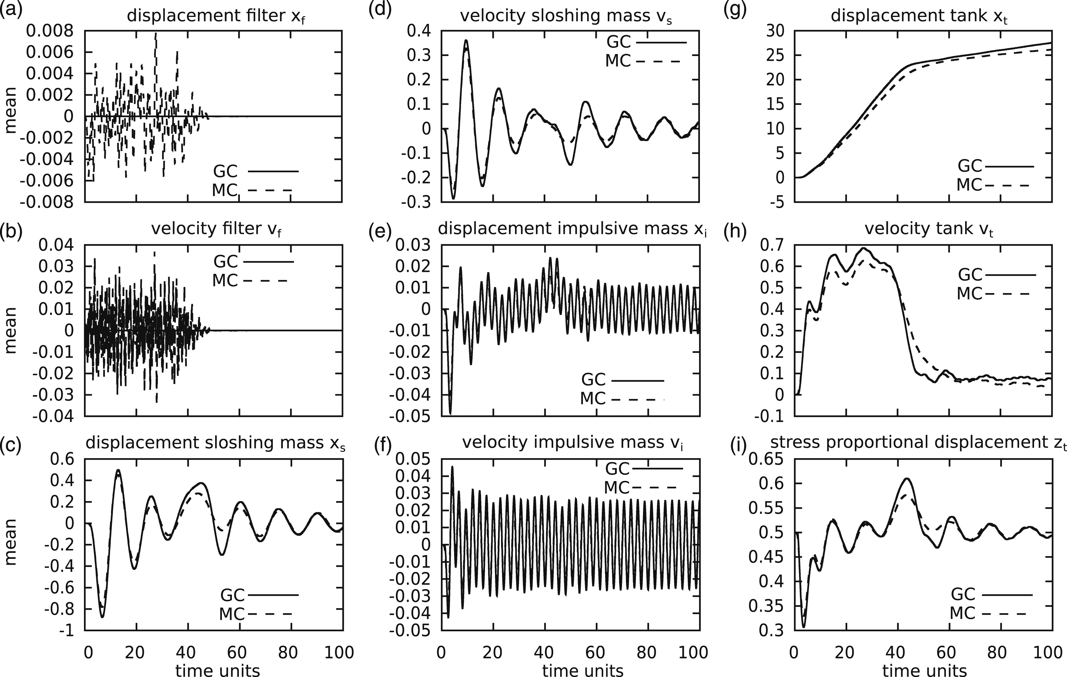
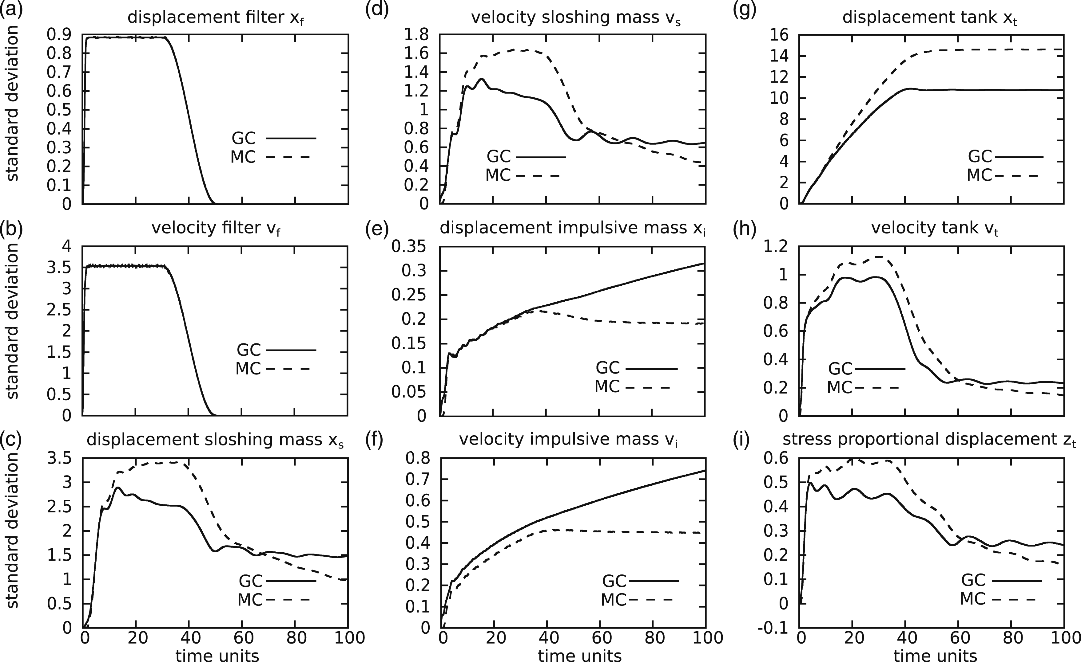
In Figure 9, the absolute displacements for the tank, the sloshing, and the impulsive mass are presented. The results from the Gaussian closure technique fit to some extent to the results from the Monte Carlo simulation. It becomes visible that the displacement of the tank dominates. In Figure 10, the mean values are reproduced and in Figure 11, the standard deviation of all state vector variables is reproduced. While the mean values of the structure are reproduced almost exactly, the standard deviations show larger differences also caused by the added noise at the DOFs, because in this section, no ground vibration is present anymore. In Figure 12, the mean values and the standard deviation of z_t are presented. Here, the effect of the small random excitation added to the system becomes visible because the attenuation is not as strong as it is in the Monte Carlo simulation.

Figure 9.

Solution for windowed colored noise (K_t = 0.5, z₀ = 0.5): Absolute displacements of the tank (t), the impulsive mass (i), and the sloshing mass (s). Presented are the mean values (M) and the mean values ± standard deviation (M ± S) for the Gaussian closure method (GC) and the Monte Carlo simulation (MC).

Figure 10.

Solution for windowed colored noise (K_t = 0.5, z₀ = 0.5): Mean values of displacement (x), velocities (v), and stress proportional displacements (z) of the filter (f), the tank (t), the impulsive mass (i), and the sloshing mass (s) for the Gaussian closure method (GC) and the Monte Carlo simulation (MC).

Figure 11.

Solution for windowed colored noise (K_t = 0.5, z₀ = 0.5): Standard deviations of displacement (x), velocities (v), and stress proportional displacements (z) of the filter (f), the tank (t), the impulsive mass (i), and the sloshing mass (s) for the Gaussian closure method (GC) and the Monte Carlo simulation (MC).

Figure 12.

Solution for windowed colored noise (K_t = 0.5, z₀ = 0.5): Force proportional displacement z. Presented are the mean values (M) and the mean values ± standard deviation (M ± S) for the Gaussian closure method (GC) and the Monte Carlo simulation (MC).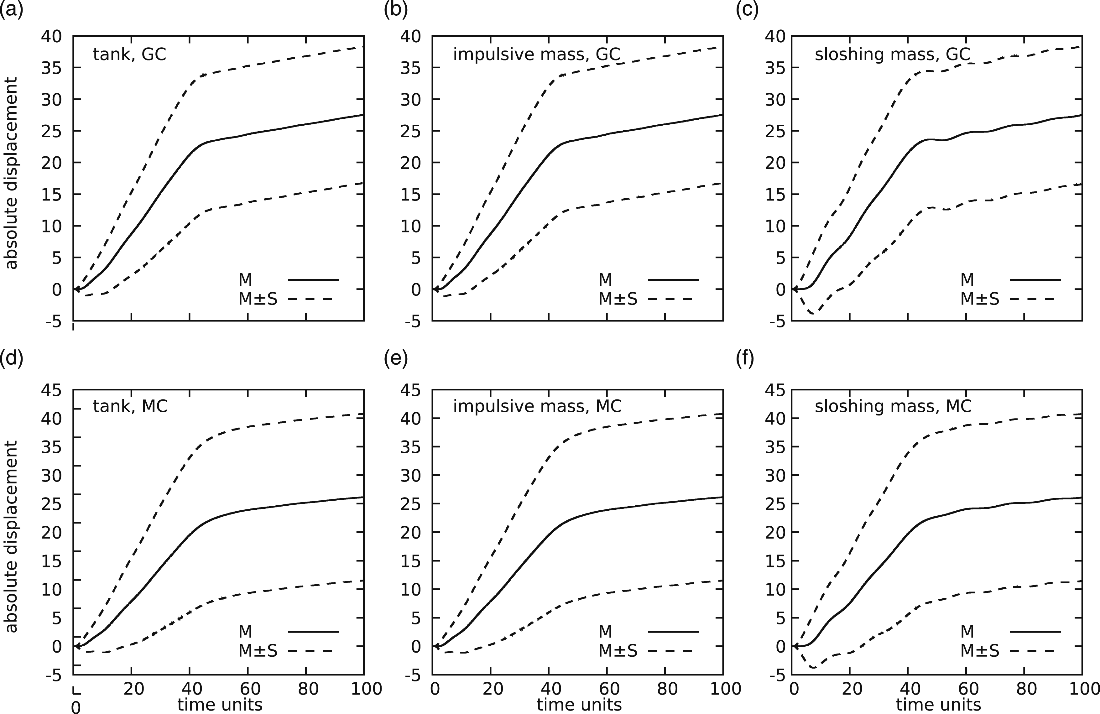

To reduce the influence of the additional noise on the DOFs in a second attempt, the same time window is used for the ground acceleration and the additional noises. This stabilization is appropriate as long as the load intensity K₀ is not too high. In Figure 13, the absolute displacements for the tank, the sloshing, and the impulsive mass are presented. The results from the Gaussian closure technique fit well to the results from the Monte Carlo simulation. Again, the displacement of the tank dominates. In Figure 14, the mean values are shown and in Figure 15, the standard deviation of all state vector variables is shown. In Figure 16, the mean values and the standard deviation of z_t are presented. Now the standard deviation of the Gaussian closure coincides better with the value of the Monte Carlo simulation in the second part without ground motion. Overall the standard deviation is slightly underestimated by the Gaussian closure for the extremely high ground motion with respect to the elasto-plastic range of [−1, 1]. The new algorithm for the MDOF case is stable enough to allow for the case without an elastic restoring force. In this case, the system is freely floating on the elasto-plastic components and there is no guarantee that stationarity will be reached.

Figure 13.

Solution for windowed stabilizing noise (K₀ = 0.5, z₀ = 0.5): Absolute displacements of the tank (t), the impulsive mass (i), and the sloshing mass (s). Presented are the mean values (M) and the mean values ± standard deviation (M ± S) for the Gaussian closure method (GC) and the Monte Carlo simulation (MC).

Figure 14.

Solution for windowed stabilizing noise (K₀ = 0.5, z₀ = 0.5): Mean values of displacement (x), velocities (v), and stress proportional displacements (z) of the filter (f), the tank (t), the impulsive mass (i), and the sloshing mass (s) for the Gaussian closure method (GC) and the Monte Carlo simulation (MC).

Figure 15.

Solution for windowed stabilizing noise (K₀ = 0.5, z₀ = 0.5): Standard deviations of displacement (x), velocities (v), and stress proportional displacements (z) of the filter (f), the tank (t), the impulsive mass (i), and the sloshing mass (s) for the Gaussian closure method (GC) and the Monte Carlo simulation (MC).

Figure 16.

Solution for windowed stabilizing noise (K₀ = 0.5, z₀ = 0.5): Force proportional displacement z. Presented are the mean values (M) and the mean values ± standard deviation (M ± S) for the Gaussian closure method (GC) and the Monte Carlo simulation (MC).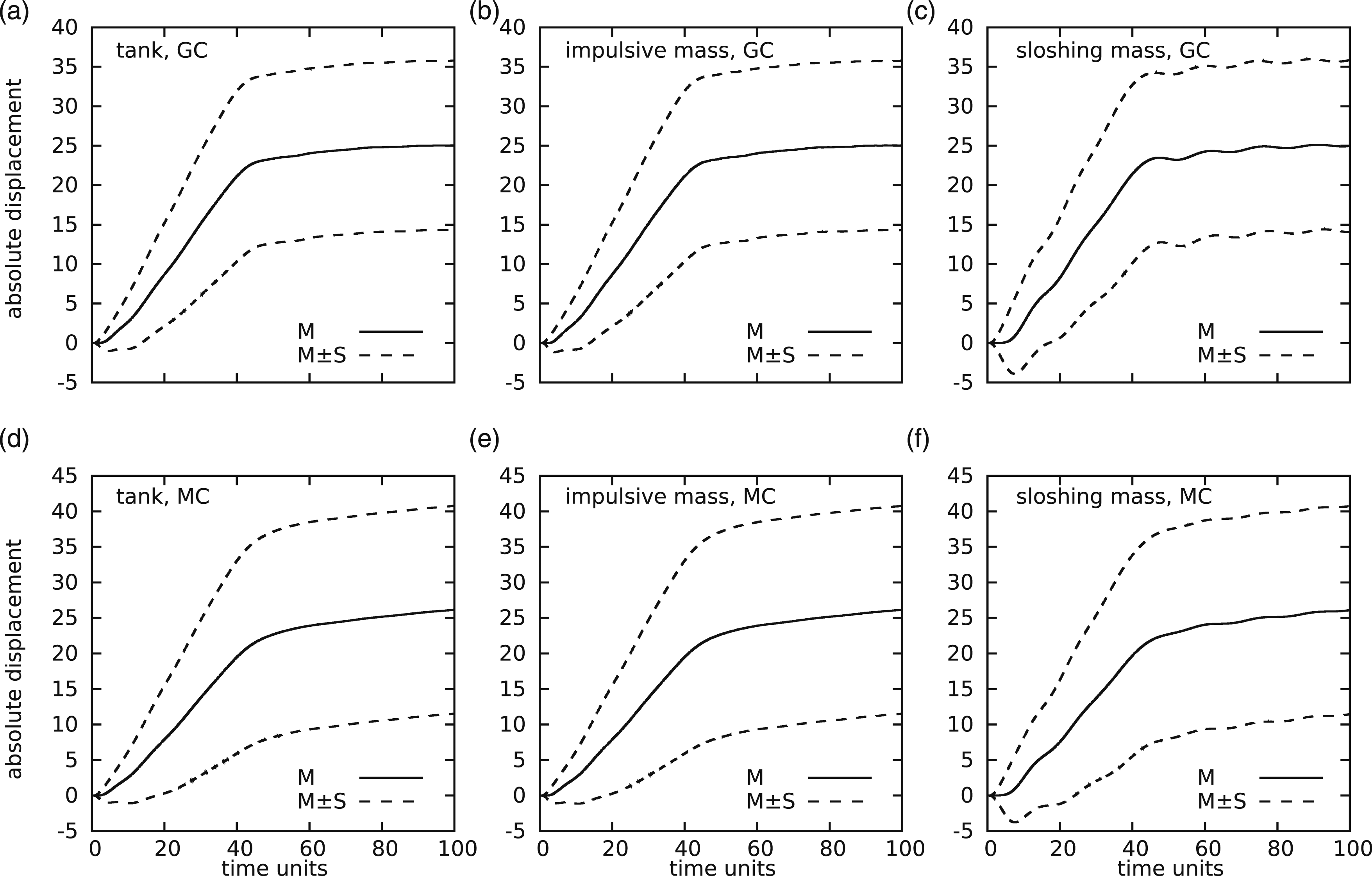

Concerning the computational cost, the time for the Gaussian closure technique is 871 s and for the Monte Carlo simulation 7474s. The Gaussian closure technique is thus 8.6 times faster than the Monte Carlo simulation using the same time step. With an adaptive time stepping, the Gaussian closure technique could be even faster and probably the deviation to the Monte Carlo simulation could be reduced.

Tank model with absolute degree of freedoms

It is possible to use absolute mechanical degree of freedoms for the sloshing mass and the impulsive mass, because they behave linear:

\begin{array}{c} \frac{\partial}{\partial t} u_{1} = u_{2}, \\ \frac{\partial}{\partial t} u_{2} = - \frac{c_{f}}{m_{f}} u_{2} - \frac{k_{f}}{m_{f}} u_{1} + \frac{ξ_{f}}{m_{f}}, \\ \frac{\partial}{\partial t} u_{3} = u_{4}, \\ \frac{\partial}{\partial t} u_{4} = - \frac{c_{s}}{m_{s}} (u_{4} - u_{8}) - \frac{k_{s}}{m_{s}} (u_{3} - u_{7}) + \frac{ξ_{s}}{m_{s}}, \\ \frac{\partial}{\partial t} u_{5} = u_{6}, \\ \frac{\partial}{\partial t} u_{6} = - \frac{c_{i}}{m_{i}} (u_{6} - u_{8}) - \frac{k_{i}}{m_{i}} (u_{5} - u_{7}) + \frac{ξ_{i}}{m_{i}}, \\ \frac{\partial}{\partial t} u_{7} = u_{8}, \\ \frac{\partial}{\partial t} u_{8} = - \frac{c_{t}}{m_{t}} u_{8} - \frac{k_{t}}{m_{t}} α_{t} u_{7} - \frac{k_{t}}{m_{t}} (1 - α_{t}) (u_{9} - z_{0}) + \frac{ξ_{t}}{m_{t}} + \\ + \frac{c_{s}}{m_{t}} (u_{4} - u_{8}) + \frac{k_{s}}{m_{t}} (u_{3} - u_{7}) + \\ + \frac{c_{i}}{m_{t}} (u_{6} - u_{8}) + \frac{k_{i}}{m_{t}} (u_{5} - u_{7}) - u_{1}, \\ \frac{\partial}{\partial t} u_{9} = A u_{8} - u_{8} u_{9} (γ sgn (u_{8}) + θ sgn (u_{9})) . \end{array}

(29)

The moment equation for this case is given by

\begin{array}{l} \frac{\partial}{\partial t} m_{\dots} = a_{1} m_{a_{1} - 1, a_{2} + 1 \dots} - \\ - \frac{c_{f}}{m_{f}} a_{2} m_{\dots} - \frac{k_{f}}{m_{f}} a_{2} m_{a_{1} + 1, a_{2} - 1 \dots} + \frac{K_{f}}{2 m_{f}^{2}} a_{2} (a_{2} - 1) m_{\dots a_{2} - 2 \dots} + \\ + a_{3} m_{\dots a_{3} - 1, a_{4} + 1 \dots} - \\ - \frac{c_{s}}{m_{s}} a_{4} m_{\dots} - \frac{k_{s}}{m_{s}} a_{4} m_{\dots a_{3} + 1, a_{4} - 1 \dots} + \frac{K_{s}}{2 m_{s}^{2}} a_{4} (a_{4} - 1) m_{\dots a_{4} - 2 \dots} + \\ + \frac{c_{t}}{m_{t}} a_{4} m_{\dots a_{4} - 1 \dots a_{8} + 1 \dots} + \frac{k_{t}}{m_{t}} α_{t} a_{4} m_{\dots a_{4} - 1 \dots a_{7} + 1 \dots} - \\ - \frac{k_{t}}{m_{t}} (1 - α_{t}) (a_{4} m_{\dots a_{4} - 1 \dots a_{9} + 1 \dots} - z_{0} a_{4} m_{\dots a_{4} - 1 \dots}) - \\ - \frac{c_{s}}{m_{t}} a_{4} m_{\dots} - \frac{k_{s}}{m_{t}} a_{4} m_{\dots a_{3} + 1, a_{4} - 1 \dots} - \frac{c_{i}}{m_{t}} a_{4} m_{\dots a_{4} - 1 \dots a_{6} + 1 \dots} - \frac{k_{i}}{m_{t}} a_{4} m_{\dots a_{4} - 1, a_{5} + 1 \dots} + \\ + a_{5} m_{\dots a_{5} - 1, a_{6} + 1 \dots} - \\ - \frac{c_{i}}{m_{i}} a_{6} m_{\dots} - \frac{k_{i}}{m_{i}} a_{6} m_{\dots a_{5} + 1, a_{6} - 1 \dots} + \frac{K_{i}}{2 m_{i}^{2}} a_{6} (a_{6} - 1) m_{\dots a_{6} - 2 \dots} + \\ + \frac{c_{t}}{m_{t}} a_{6} m_{\dots a_{6} - 1 \dots a_{8} + 1 \dots} + \frac{k_{t}}{m_{t}} α_{t} a_{6} m_{\dots a_{6} - 1, a_{7} + 1 \dots} - \\ - \frac{k_{t}}{m_{t}} (1 - α_{t}) (a_{6} m_{\dots a_{6} - 1 \dots a_{9} + 1 \dots} - z_{0} a_{6} m_{\dots a_{6} - 1 \dots}) - \\ - \frac{c_{s}}{m_{t}} a_{6} m_{\dots a_{4} + 1 \dots a_{6} - 1 \dots} - \frac{k_{s}}{m_{t}} a_{6} m_{\dots a_{3} + 1 \dots a_{6} - 1 \dots} - \frac{c_{i}}{m_{t}} a_{6} m_{\dots} - \frac{k_{i}}{m_{t}} a_{6} m_{\dots a_{5} + 1, a_{6} - 1 \dots} + a_{7} m_{\dots a_{7} - 1, a_{8} + 1 \dots} - \\ - \frac{c_{t}}{m_{t}} a_{8} m_{\dots} - \frac{k_{t}}{m_{t}} α_{t} a_{8} m_{\dots a_{7} + 1, a_{8} - 1 \dots} - \\ - \frac{k_{t}}{m_{t}} (1 - α_{t}) (a_{8} m_{\dots a_{8} - 1, a_{9} + 1 \dots} - z_{0} a_{8} m_{\dots a_{8} - 1 \dots}) + \\ + \frac{c_{s}}{m_{t}} a_{8} m_{\dots a_{4} + 1 \dots a_{8} - 1 \dots} + \frac{k_{s}}{m_{t}} a_{8} m_{\dots a_{3} + 1 \dots a_{8} - 1 \dots} + \frac{c_{i}}{m_{t}} a_{8} m_{\dots a_{6} + 1 \dots a_{8} - 1 \dots} + \\ + \frac{k_{i}}{m_{t}} a_{8} m_{\dots a_{5} + 1 \dots a_{8} - 1 \dots} + \frac{K_{t}}{2 m_{t}^{2}} a_{8} (a_{8} - 1) m_{\dots a_{8} - 2 \dots} - a_{8} m_{\dots a_{1} + 1 \dots a_{8} - 1 \dots} + \\ + A a_{9} m_{\dots a_{8} + 1, a_{9} - 1 \dots} - \\ - γ a_{9} \int_{- \infty}^{\infty} \dots \int_{- \infty}^{\infty} \dots u_{8}^{a_{8} + 1} \dots s g n (u_{8}) p (u) d u - \\ - θ a_{9} \int_{- \infty}^{\infty} \dots \int_{- \infty}^{\infty} \dots u_{8}^{a_{8} + 1} \dots s g n (u_{9}) p (u) d u . \end{array}

(30)

The results for this case are the same as before, but the model is more sensitive to zero values of the window attenuating the load. Therefore, a window was used that results in a residual excitation:

ξ_{w} (t) = {\begin{array}{c} 0.1, & t < t_{0} \\ \frac{1}{2} \cdot (1 - \cos (π \cdot \frac{t - t_{0}}{t_{1} - t_{0}})) \cdot 0.9 + 0.1, & t_{0} \leq t \leq t_{1} \\ 1, & t_{1} < t < t_{2} \\ \frac{1}{2} \cdot (1 - \cos (π \cdot \frac{t_{3} - t}{t_{3} - t_{2}})) \cdot 0.9 + 0.1, & t_{2} \leq t \leq t_{3} \\ 0.1, & t_{3} < t . \end{array}

(31)

For this window, no additional noises have to be added to the DOFs. The results using this window are better than before because less corrections of zero variances are needed. The following parameters were used:

• total time is 100, step size is 10⁻⁴,

• tank: m_t = 1.0, c_t = 0.0, k_t = 1.0, α_t = 0.0, A = 1.0, γ = 0.5, θ = 0.5, z₀ = 0.0,

• impulsive mass: m_i = 1.0, c_i = 0.0, k_i = 0.5,

• swapping mass: m_s = 0.5, c_s = 0.0, k_s = 0.1,

• filter: m_f = 0.06667, c_f = 0.3, k_f = 1.06667, K₀ = 0.02.

The results are presented in Figures 17–20. It is visible that the agreement of the Monte Carlo simulation and the Gaussian closure method is good. Therefore, it becomes clear now that the behavior of the linear filter is crucial for the results of the Gaussian closure. If the noise tends to zero, the state vector variables belonging to the filter also tend to zero, because the filter is a highly damped oscillator that tends quickly towards zero, if no load is present. These zeros lead to a covariance matrix that is no more positive definite and not invertible. To avoid this, a minimum variance is introduced instead of zeros or slightly negative values in the main diagonal of the matrix. This correction leads to differences compared to the Monte Carlo simulation. The mean values exhibit a time delay for the Gaussian closure method that is not present in the Monte Carlo method. The reason for this behavior is unclear.

Figure 17.

Absolute DOFs with (K₀ = 0.02, z₀ = 0.0): Absolute displacements of the tank (t), the impulsive mass (i), and the sloshing mass (s). Presented are the mean values (M) and the mean values ± standard deviation (M ± S) for the Gaussian closure method (GC) and the Monte Carlo simulation (MC).

Figure 18.

Absolute DOFs with (K₀ = 0.02, z₀ = 0.0): Mean values of displacement (x), velocities (v), and stress proportional displacements (z) of the filter (f), the tank (t), the impulsive mass (i), and the sloshing mass (s) for the Gaussian closure method (GC) and the Monte Carlo simulation (MC).

Figure 19.

Absolute DOFs with (K₀ = 0.02, z₀ = 0.0): Standard deviations of displacement (x), velocities (v), and stress proportional displacements (z) of the filter (f), the tank (t), the impulsive mass (i), and the sloshing mass (s) for the Gaussian closure method (GC) and the Monte Carlo simulation (MC).

Figure 20.

Absolute DOFs with (K₀ = 0.02, z₀ = 0.0): Force proportional displacement z. Presented are the mean values (M) and the mean values ± standard deviation (M ± S) for the Gaussian closure method (GC) and the Monte Carlo simulation (MC).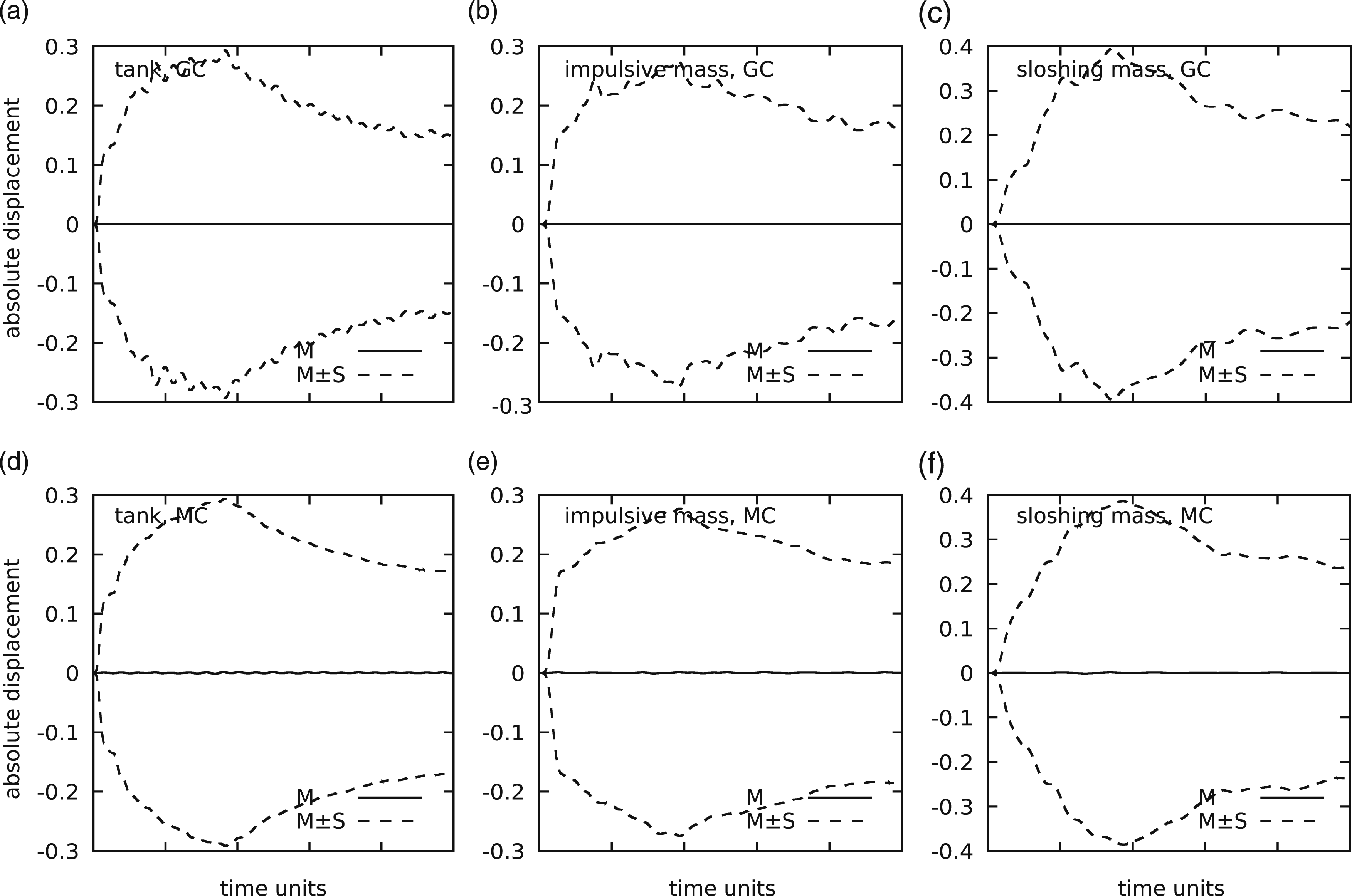

The processing time on a new Core-i7 computer (i7-8700) is for the Gaussian closure 277 s and for the Monte Carlo method 5664 s. The Gaussian closure is thus 20 times faster than the Monte Carlo method.

The same case with an offset z₀ = 0.1 is presented in Figures 21–24 for absolute coordinates. The stabilizing white noise processes are set to zero: K_t = K_s = K_i = 0.

Figure 21.

Absolute DOFs with (K₀ = 0.02, z₀ = 0.1): Absolute displacements of the tank (t), the impulsive mass (i), and the sloshing mass (s). Presented are the mean values (M) and the mean values ± standard deviation (M ± S) for the Gaussian closure method (GC) and the Monte Carlo simulation (MC).

Figure 22.

Absolute DOFs with (K₀ = 0.02, z₀ = 0.1): Mean values of displacement (x), velocities (v), and stress proportional displacements (z) of the filter (f), the tank (t), the impulsive mass (i), and the sloshing mass (s) for the Gaussian closure method (GC) and the Monte Carlo simulation (MC).

Figure 23.

Absolute DOFs with (K₀ = 0.02, z₀ = 0.1): Standard deviations of displacement (x), velocities (v), and stress proportional displacements (z) of the filter (f), the tank (t), the impulsive mass (i), and the sloshing mass (s) for the Gaussian closure method (GC) and the Monte Carlo simulation (MC).

Figure 24.

Absolute DOFs with (K₀ = 0.02, z₀ = 0.1): Force proportional displacement z. Presented are the mean values (M) and the mean values ± standard deviation (M ± S) for the Gaussian closure method (GC) and the Monte Carlo simulation (MC).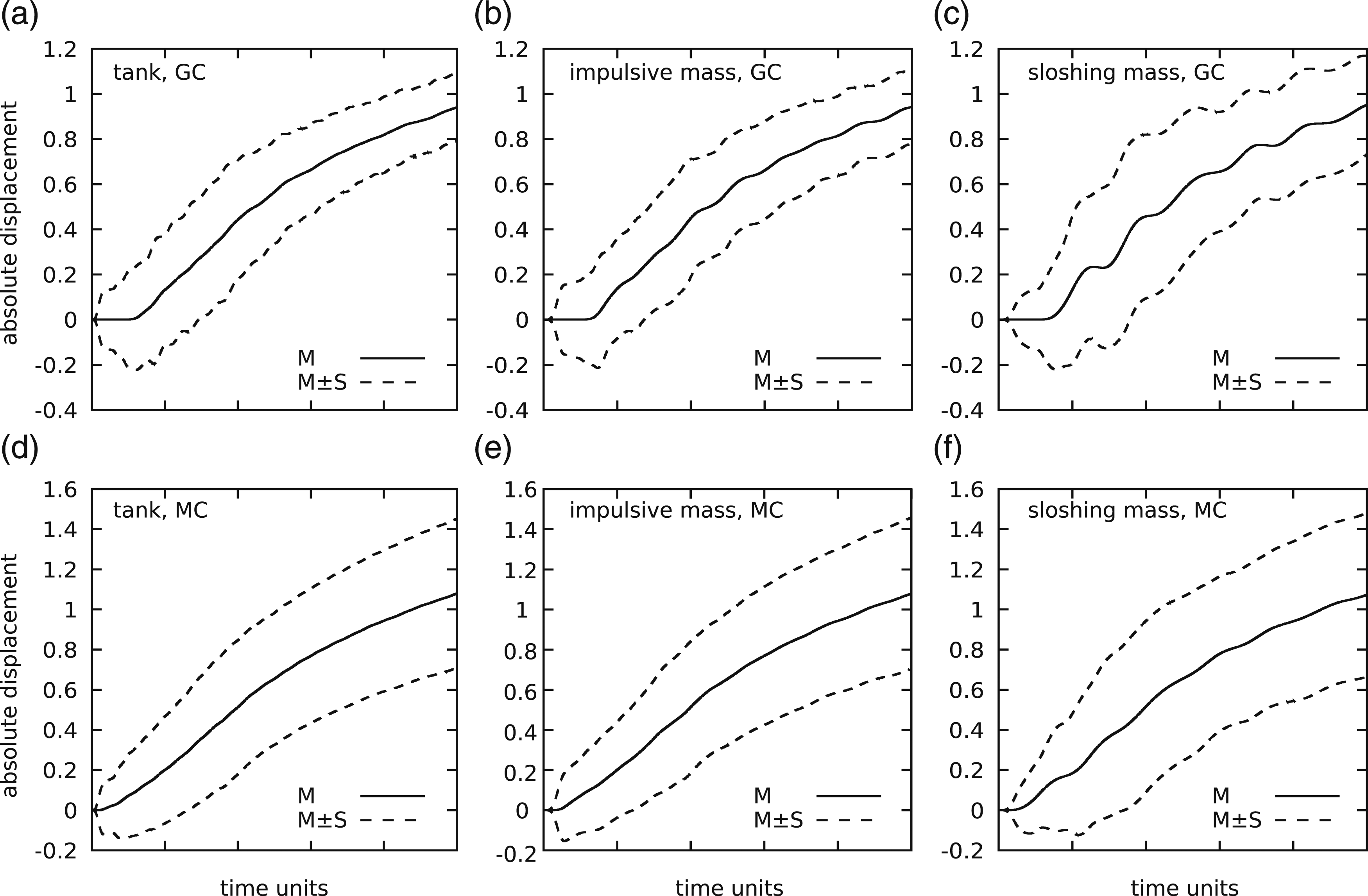

For comparison, the results for the case with relative coordinates and z₀ = 0.1 are given in Figures 25–28. In Figure 29, the histograms for the Monte Carlo method and the Gaussian distributions from the closure method are compared. The deviations increase with time and in particular the tank variables but also v_i deviate. x_t also exhibits some skewness with a heavier tail toward higher values.

Figure 25.

Relative DOFs with (K₀ = 0.02, z₀ = 0.1): Absolute displacements of the tank (t), the impulsive mass (i), and the sloshing mass (s). Presented are the mean values (M) and the mean values ± standard deviation (M ± S) for the Gaussian closure method (GC) and the Monte Carlo simulation (MC).

Figure 26.

Relative DOFs with (K₀ = 0.02, z₀ = 0.1): Mean values of displacement (x), velocities (v), and stress proportional displacements (z) of the filter (f), the tank (t), the impulsive mass (i), and the sloshing mass (s) for the Gaussian closure method (GC) and the Monte Carlo simulation (MC).

Figure 27.

Relative DOFs with (K₀ = 0.02, z₀ = 0.1): Standard deviations of displacement (x), velocities (v), and stress proportional displacements (z) of the filter (f), the tank (t), the impulsive mass (i), and the sloshing mass (s) for the Gaussian closure method (GC) and the Monte Carlo simulation (MC).

Figure 28.

Relative DOFs with (K₀ = 0.02, z₀ = 0.1): Force proportional displacement z. Presented are the mean values (M) and the mean values ± standard deviation (M ± S) for the Gaussian closure method (GC) and the Monte Carlo simulation (MC).

Figure 29.

Relative DOFs with (K₀ = 0.02, z₀ = 0.1): Histogram of displacement (x), velocities (v), and stress proportional displacements (z) of the filter (f), the tank (t), the impulsive mass (i), and the sloshing mass (s) for the Gaussian closure method (GC) and the Monte Carlo simulation (MC) at 10 and 100 time units. Kurtosis (k) and skewness (s) are given for the Monte Carlo results. The Gaussian distributions have a kurtosis of 3 and a skewness of 0.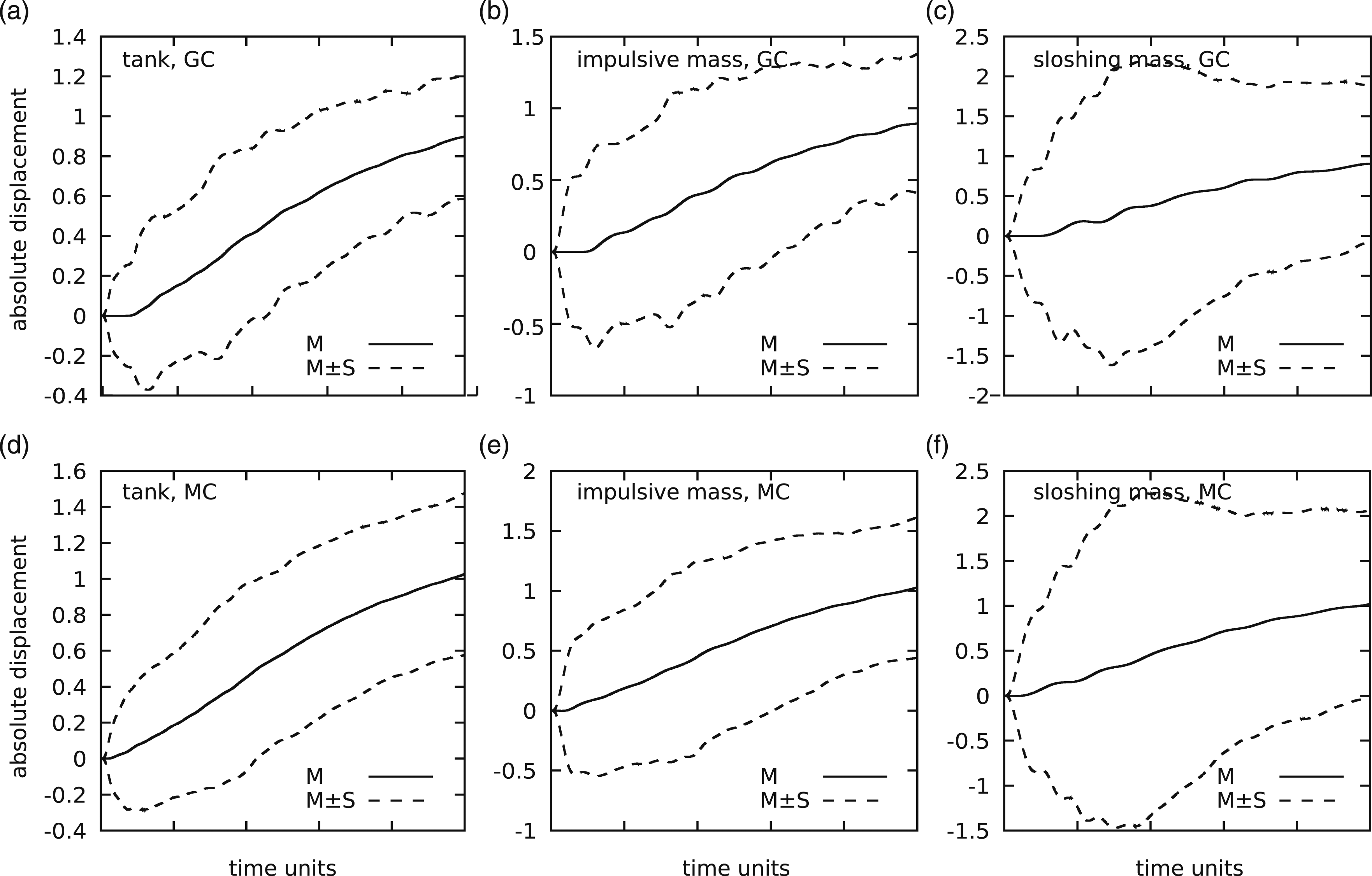

The processing time on a Core-i7 computer (i7-8700) is for the Gaussian closure 252 s and for the Monte Carlo method 5768 s. The Gaussian closure is 23 times faster than the Monte Carlo method. The decrease in the computational time is probably caused by a reduced need for stabilization measures.

The method with relative degrees of freedom behaves more stable than the method with absolute degrees of freedom. The reason is that in the relative case, the displacements are much less correlated with one another and high correlation factors require stabilization measures.

Both examples were also tested with the explicit Runge–Kutta RK4 integration scheme, but both cases lead to instabilities. Therefore, no results can be presented here. Additionally, the implicit Radau method was tested. It runs until 4.9 time units for the absolute variables and about 10 time units for the relative variables. The Radau method becomes probably unstable because numerical derivatives are used.

Conclusions

A Gaussian closure method for a three degree-of-freedom model for a tank was developed that uses a time step procedure to calculate the transient response to a system under stochastic excitation for the elasto-plastic case. The model allows for a dead load and thus non-zero mean which can also be interpreted as a non-symmetric hysteresis of the support of the tank. A low-pass filtered white noise ground acceleration was the original input on the system. Additionally, the intensity of the ground motion was assumed to be time dependent using an asymmetrical tapered cosine window.

Even for high amplitudes with respect to the limits of the elasto-plastic limit of the hysteretic element described by the original Bouc model, the results for the moments are mostly in good agreement with the results from the Monte Carlo simulation which is the reference method for stochastic non-linear systems. Clearly, for large noise levels and/or large levels of asymmetry, the Gaussian distribution fails to model the actual distribution properly due to the limits in the force proportional displacement which also affects other quantities. This limitation is to be expected from a second order moment approach based on the assumption of a multivariate Gaussian distribution. Therefore, the results cannot be used to estimate the tails of the correct distribution. The idea of the approach is to do fast parameter studies to find optimized parameters. After this first step, a detailed finite element model is needed in combination with a Monte Carlo method to approximate the extreme parts of the random distribution.

The Gaussian closure technique estimates the means and the covariances of all degrees of freedom of the system. The number of mean values grows linearly with the number of degrees of freedom, but the number of covariances increases quadratically with the number of degrees of freedom. Therefore, the approach is limited to parameter studies with a small number of degrees of freedom. In methods based on the Fokker–Planck–Kolmogorov equation, the dimension of the multivariate distribution is linearly coupled with the number of degrees of freedom of the system. As a consequence, the Monte Carlo methods are better suited for a large number of degrees of freedom.

Another issue is that for the impulsive mass of the fluid, a relatively high resonance frequency was assumed. This leads to instabilities in the algorithm because coherent behavior of several state vector variables occurs, which results in problems with the analytic integration for moments of the Gaussian closure technique.

Difficulties also arise for the linear filter with high damping values. When the load is set to zero (i.e., outside of the load window), the variances of the state vector variables of the filter tend to zero and the Gaussian distribution becomes a Dirac delta distribution that cannot be handled by the integration procedure. Therefore, several measures were introduced to stabilize the equations. One approach was to apply a small additional white noise to every degree of freedom either unweighted or weighted by the window used for the load. The time windowing was shown to be important to avoid inaccuracies for small excitation amplitudes. Another method was the usage of a small residual excitation noise. Here it was found that about 10% of the maximum amplitude is needed to reach stability. Otherwise, the state vector variables of the linear filter tend to zero which causes a semi-definite covariance matrix that cannot be inverted any more.

Furthermore, instead of the simple time step procedure, the explicit Runge–Kutta and the adaptive implicit Radau method were tested. These methods, however, showed even more instabilities than the simple time step method.

The assumption of a Gaussian distribution for the force proportional displacement z_t does not agree with the limits of this variable [−1,1], but the deviation of the mean value and the standard deviation with respect to the exact solution is small. Therefore, a possible method could be to fit the two moments to a beta-distribution.

Footnotes

Declaration of conflicting interests

The author(s) declared no potential conflicts of interest with respect to the research, authorship, and/or publication of this article.

Funding

The author(s) received no financial support for the research, authorship, and/or publication of this article.

ORCID iD

Holger Waubke

References

Waubke

. Moment-Closure Technik zur Abschaetzung der elasto-plastischen Reaktion von Stockwerksrahmen auf zufaellige Belastungen aus Windereignissen. Habilitation Berichte aus dem Konstruktiven Ingenieurbau TU Muenchen 1999; 1/99.

Bouc

. Forced vibration of mechanical systems with hysteresis. Proceedings of the Fourth Conference on Non-linear Oscillation, Prague, September 5–9 1967, 1967. (abstract).

Charalampakis

Koumousis

. On the response and dissipated energy of Bouc–Wen hysteretic model. J Sound Vibration 2008; 309: 887–895.

Charalampakis

Koumousis

. Identification of Bouc-Wen hysteretic systems by a hybrid evolutionary algorithm. J Sound Vibration 2008; 314: 571–585.

Ehrlicher

Point

. Thermodynamic admissibility of Bouc-Wen type hysteresis models. Comptes Redus – Mechanique 2004; 332(1): 51–57.

Giaralis

Spanos

. Derivation of equivalent linear properties of Bouc-Wen hysteretic systems for seismic response spectrum analysis via statistical linearization. In: 10th HSTAM International Congress on Mechanics, Chania, Crete, Greece, 2013. (CD–ROM).

Hurtado

Barbat

. Equivalent linearization of the Bouc-Wen hysteretic model. Eng Struct 2000; 22: 1121–1132.

Ismail

Ikhouane

Rodellar

. The hysteresis Bouc-Wen model, a survey. Arch Comput Methods Eng 2009; 16: 161–188.

Lin

Kozin

Wen

, et al. Methods of stochastic structural dynamics. Struct Saf 1986; 3: 167–194.

10.

Wen

. Method for random vibration of hysteretic systems. J Eng Mech Division 1976; 102(2): 249–263.

11.

Wen

. Equivalent linearization for hysteretic systems under random excitation. J Appl MechanicsASME 1980; 47: 150–154.

12.

Baber

Noori

. Random vibration of degrading, pinching systems. J Eng Mech 1985; 111(8): 1010–1026.

13.

Suzuki

Minai

. Application of stochastic differential equations to seismic reliability analysis of hysteretic structures. Probabilistic Eng Mech 1988; 3(1): 43–52.

14.

AAloisio

Köhler

, et al. Extension of generalized Bouc-Wen hysteresis modeling of wood joints and structural systems. J Eng Mech 2020; 146146(33): 0420001.

15.

Roberts

Spanos

. Random vibration and statistical linearization. New York, NY: Dover Publications Minela, 2003.

16.

Spanos

Giaralis

. Third-order statististical linearization-based approach to derive equivalent linear properties of bilinear hysteretic systems for seismic response spectrum analysis. Struct Saf 2013; 44: 59–69.

17.

Pradlwarter

Schueller

. Accuracy and limitations of the method of equivalent linearization for hysteretic multi-storey frames. In: Nonlinear stochastic dynamic engineering systems. Austria: IUTAM Symposium Innsbruck/Igls, pp. 3–21.

18.

Sett

Jeremic

Kavvas

. Stochastic elastic-plastic finite elements. Comput Methods Appl Mech Eng 2011; 200: 997–1007.

19.

Ghanem

Spanos

. Stochastic finite elements: A spectral approach. Ney Work, NY. Springer-Verlag New York, 1991.

20.

Narayanan

Kumar

. Numerical solutions of Fokker-Planck equation of nonlinear systems subjected to random harmonic excitations. Probabilistic Engineering Mechanics 2012; 27: 35–46.

21.

Chen

. The probability density evolution method for dynamic resposne analysis of non-linear stochatsic structures. Int J Numerical Methods Eng 2006; 65: 882–903.

22.

Caughey

Dienes

. Analysis of a nonlinear first-order system with a white noise input. J Appl Phys 1961; 33(11): 2476–2479.

23.

Waubke

Kasess

. Berechnung hysteretischer Elemente ohne elastische Rueckstellkraft. In: Fortschritte in der Akustik DAGA 2017. Kiel. (CD–ROM).

24.

Waubke

Kasess

. Gaussian closure technique fo chain like structures with elasto-plastic elements described by the bouc hysteresis. J Sound Vibration 2017; 382: 73–86.

25.

Waubke

Kasess

. Transient response of one degree of freedom systems with bouc-hysteresis excited by white noise. Proced Eng 2017; 199: 1146–1151.

26.

Ibrahim

Soundarajan

. Non-linear parametric liquid sloshing under wide band random excitation. J Sound Vibration 1983; 91(1): 119–134.

27.

Isserlis

. On certain probable errors and correlation coefficients of multiple frequency distributions with skew regression. Biometrika 1916; 11: 185–190.

28.

Isserlis

. On a formula for the product-moment coefficient of any order of a normal frequency distribution in any number of variables. Biometrika 1918; 12: 134–139.

29.

Waubke

Kasess

. Gaussian closure technique applied to the hysteretic bouc model with non-zero mean white noise excitation. J Sound Vibration 2016; 382: 258–273.

30.

Algreane

Osman

Karim

, et al. Behavior of elevated concrete water tank subjected to artificial ground motion. Electron J Geotechnical Eng 2011; 16: 387–406.

31.

Karavasilis

Rizos

Karabalis

. Seismic analysis of spherical tanks including fluid-structure-soil interaction. In: 13th World Conference on Earthquake Engineering, Vancouver, Canada, August 1–6 2004, 2004; 1814. pp. 1–15.

32.

Shakib

Alemzadeh

. The effect of earthquake site-source distance on dynamic response of concrete elevated water tanks. Proced Eng 2017; 199: 260–265.

33.

Mangulkar

Madhukar

. Review on seismic analysis of elevated water tank. Int J Civil Eng Technol (IJCIET) 2013; 4(2): 288–294.

34.

Walde

Manchalwar

Khedikar

. Seismic analysis of water tank considering effect on time period. Int J Res Eng Technol (IJRET) 2015; 4(6): 284–288.

35.

Omidinasab

Shakib

. Seismic response evaluation of the rc elevated water tank with fluid-structure interaction and earthquake ensemble. KSCE J Civil Eng 2012; 16(3): 276–366.

36.

Kolmogorov

. Ueber die analytischen methoden in der wahrscheinlichkeitsrechnung. Mathematische Annalen 1931; 104: 415–458.

37.

Kasess

Waubke

. Bouc hysteresis under white noise excitation using non-linear mapping and the beta distribution. J Theor Comput Acoust Spec Issue AFBEM 2018; 26(03): 1850042.

Gaussian closure technique for a simple tank model with non-zero mean random load and elasto-plasticity

Abstract

Keywords

Introduction

Multi-degree of freedom model of a tank

Results for a tank under filtered white noise excitation

Tank model with absolute degree of freedoms

Conclusions

Footnotes

Declaration of conflicting interests

Funding

ORCID iD

References