Sage Journals: Discover world-class research

Abstract

With the development of modern industrial technology, it is an essential problem to calculate the noise reduction performance of the flexible partition walls. The sound insulation measurement model is modeled by the Spectral geometry method (SGM). Compared with the traditional ones, it is a method with higher calculation accuracy and faster convergence speed. The displacement of the panel and the sound pressure field inside the rooms are expressed as Fourier series with additional items. In order to simulate the real measurement environment, the sound source room and the receiving room are set as a reverberation chamber and an anechoic chamber with impedance boundaries, respectively. The coupling relationship is established by the Hamilton’s principle. Then the natural frequencies and the sound pressure level are compared with those derived by the finite element method (FEM). The results show that the analytical method has good accuracy and convergence. Moreover, the sound transmission loss (STL) of the partition could be obtained by the sound pressure method. Considering there is no accurate method for measuring the STL, this paper studies some factors affecting the sound insulation performance of the model by the parametric analysis method, such as the thickness of the panel, the length of the receiving room, the impedance of the receiving room and the parameters of medium.

Keywords

Spectral geometry method Plate structure Reverberation chamber Sound insulation Sound intensity

Introduction

Sound insulation refers to the use of sound insulation structures such as sound insulation walls and light composite structures to shield sound energy, so as to reduce the harm of noise and sound radiation. Therefore, sound insulation testing technology is of great significance to improving the quality of human life and the development of industrial engineering. Compared with the field experiment, a virtual one is easier to realize and less disturbed by external factors and it is convenient for parametric analysis under different circumstances. The virtual testing is also a meshless method, which can provide faster computing speed with the same accuracy. The study of the coupling cavities is also able to provide effective theoretical guidance for the design of structures and noise control in practical engineering.

Fourier series method has been proposed, where the physical field is represented as a combination of Fourier series and supplementary expansions to give a guarantee that the sound pressure is continuous on any boundary.¹ The impedance distribution function on each surface is expressed as an energy term in the Lagrange equation of the cavity.² A unified scheme was also proposed for the treatment of plates with turbulent boundary layers.³ The modal parameters of the cavity are able to be obtained simultaneously by solving the eigenvalue problem of the standard matrix, rather than iteratively solving the nonlinear transcendental equation.⁴ Besides of this, the Rayleigh sound radiation integral equation can be used to predict the sound radiation power of the cavity-panel model when the plate is placed in an infinite barrier.⁵ The sound power was calculated in the integral form of sound pressure and normal particle velocity and a double-layer error sensing arrangement would have less impact on the sound radiation through a cavity opening.⁶ For further study of the plate with holes, Wang et al.^7–8 discussed the idea about translating the free vibration problem of a plate with holes into that of an equivalent one with no thickness. The effect of the porosity distributions in the thickness on the porous plates was also analyzed by using the geometric approach. Shi et al.^9–10 used the variational iteration method (VIM), harmonic balance method, and Lagrange energy method to derive the vibration equation of the cavity-panel system. Through numerical modeling method, Dai et al.¹¹ have discovered the coupling degree between magnon modes in a single cavity is decided by the geometric parameters of the frame member. On this basis, Chin et al.¹² developed a fully coupled panel-cavity model based on the Chebyshev–Ritz to study the influence of different structures on acoustic characteristics. A multi plate-cavity coupling model is also established by Wang et al.¹³ to investigate the effect of parameters on free vibration. Hu et al.^14–17 studied the sound radiation characteristics of common rectangular plates and complex plates based on the Hamilton differential principle. Through the Fourier series method and the energy principle, the natural modes and forced response of the U-shaped plate-cavity model under various excitation are studied.¹⁸ This method can also be used to analyze a plate backed by an irregular cavity with different boundaries when coordinate transformation technology is applied.^19–20

It is inconvenient to express the sound insulation performance of materials and components because the transmission number varies widely.^21–22 It is highly required that a relatively practical and convenient physical quantity to represent the sound insulation performance of materials and components.^23–24 The components of tests have a significant impact on the results of sound insulation, and the modes of the cavities will weaken the vibration of the structure.²⁵ Peng et al.²⁶ also found an improved semi-empirical model, which can also be used to predict the normal sound absorption coefficient of porous materials in high-frequency. The latest researches have shown that plate structures have a good effect in low-frequency, but there are still problems on how to reduce the mass of plate structure without affecting the sound insulation performance. For this purpose, Xiao et al.²⁷ proposed an analytical method to simplify the finite element model and conducted an elaborate parametric study to guide the design of parameters of the model. Oudich et al.²⁸ proposed a method based on plane wave to compute the STL for the plates. The results show that the parameters such as thickness, material, and acoustic incidence angle will all make a difference on the STL. In order to apply the principle of acoustic black holes (ABHs) in practical engineering to achieve the effect of shock absorption and noise reduction, Deng et al.²⁹ measured the sound transmission loss (STL) between two rooms by using the statistical modal energy distribution analysis (SmEdA) to study the effect of mass and stiffness.³⁰ Xiang³¹ has summarized the Sabine’s reverberation theory to make a great improvement on the measurements of incident absorption coefficients. The formula is effective only when the absorbing power is nearly uniformly distributed in the room. The ISO standard documents^32–34 provide the ways to measure the sound power level and the sound insulation of buildings and building components. Sum et al.³⁵ found a method that can get the decay time through solving the coupling between the modes under the rigid condition of the rectangular room that bounds the irregular room to study how the inclination of the wall and the impedance surface affect the reverberation time of the irregular room. Ljunggren et al.^36–37 also investigated the acoustic characteristics of the single wall rectangular room through analytical methods. The problems of the potential and kinetic energy densities of a coupling model in a steady condition is studied by Meissner et al.^38–39 through a way called the modal expansion method. They also provided a way to control the vibration and sound radiation of flexible plates through intelligent sensors.

The problems of nonlinear systems and complex structures have already been studied in various cases. He⁴⁰ found a simple way to evaluate the frequency of a nonlinear system by solving the cubic-quintic Duffing equation. Two simplified methods for the Hamiltonian-based frequency formulation are also provided by Ma,⁴¹ and the comparison between the exact solution and the approximate solution showed the accuracy of the theory. Wang et al.⁴² used the improved Fourier series method to explore the vibration problem of beams with variable cross sections. In Beauvais’s opinion,^43–44 the sound field in a panel-cavity coupling system can be divided into the purely random pressure field, the perfectly correlated pressure field, the incident diffuse field and the turbulent boundary field. For solving the vibro-acoustic problems more conveniently, the Modal Energy Analysis (MODENA) works in numerical calculation.^45–46 Kang et al.⁴⁷ evaluated the reliability of the methods to measurement noises, damping ratio of sound excitations, and harmonic excitations in simulation calculation and real field test. The modal superposition method is also applied to analyze the tire components in order to reduce the tire interior noise.⁴⁸ Stiffened plates composite structures and partially cracked plates are also the focus of current research. Based on the shear deformation theory, Shi et al.⁴⁹ proposed a coupling model combined with cylindricalconical shells and annular plates by using the energy equations. Yu et al.⁵⁰ considered the large deformation of plate-beam composite structures from the perspective of two-dimensional using the absolute nodal coordinate formulation (ANCF) method. Aiming at making the structure capable of isolating sound waves in certain frequency regions, tests on some plates were carried out to analyze their effects on the overall design.⁵¹ The experiment was carried out to find the relationship between density and sound pressure based on the acoustic gradient theory.⁵²

The references have already done lots of work on the mathematical modeling of coupling structures. However, there is no deeper exploration on the virtual measurement model from the aspect of sound insulation performance.

Theoretical formulations

Figure 1 is the coupling system composed of two acoustic cavities and the installation sketch of the rectangular panel, which is elastically restrained at the coupling surface. In this model, three sub coordinate systems of the sound source room, the receiving room, and the panel named O₁-x₁-y₁-z₁, O₂-x₂-y₂-z₂ and O₃-x₃-y₃ are established. The walls of the receiving room are set as impedance boundaries. The sound source(s) could be placed at any position(s) in the source room. The sound pressure field inside the two rooms is coupled through the plate structure. As shown in Figure 1, the dimensions of the two rooms and the panel are: L_x1 × L_y1 × L_z1, L_x2 × L_y2 × L_z2 and a × b × h.

Figure 1.

Coupled model of the sound insulation measurement suite and the panel constrained by elastic boundaries.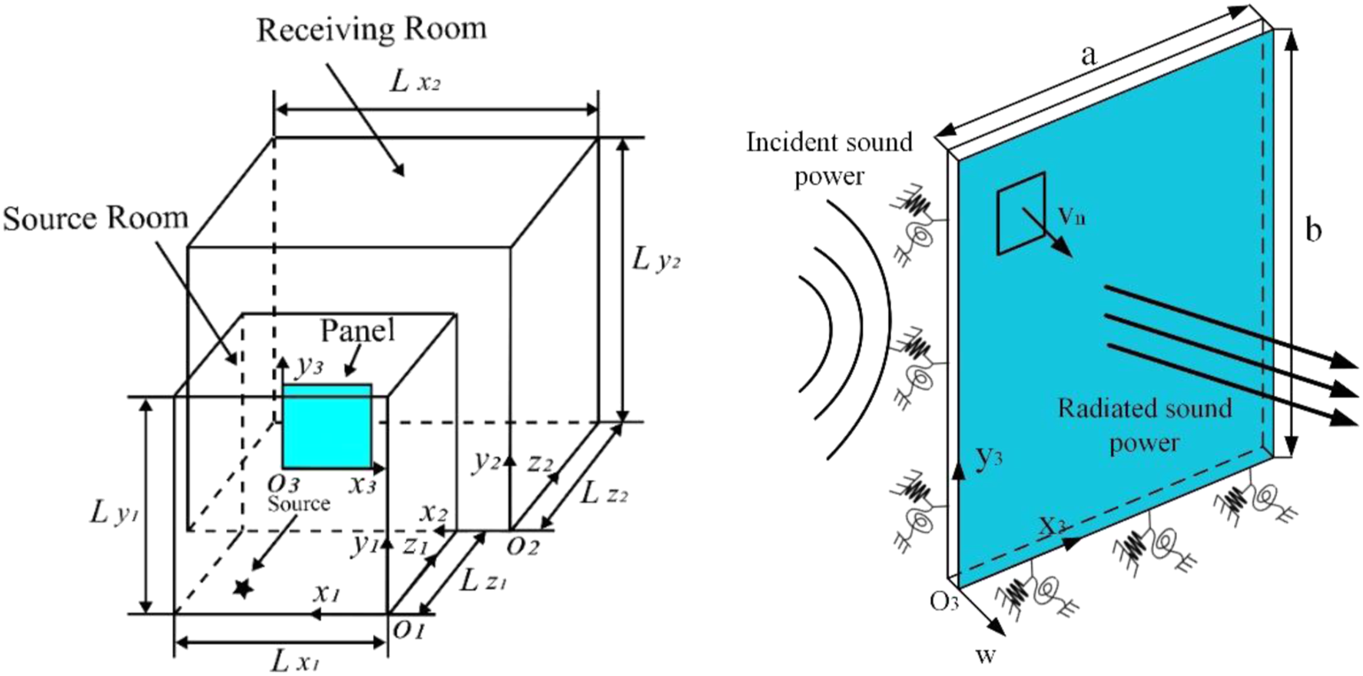

Acoustic field in the suite

According to Spectral geometry method (SGM), the sound pressure in the cavities can expressed as three-dimensional Fourier series plus additional terms. P₁ is the sound pressure in the source room and P₂ is the sound pressure in the receiving room, which can be defined as^1–2

\begin{array}{l} P_{1} (x, y, z) = \sum_{m_{x} = 0}^{M_{x 1}} \sum_{m_{y} = 0}^{M_{y 1}} \sum_{m_{z} = 0}^{M_{z 1}} P_{1 m_{x} m_{y} m_{z}} \cos λ_{m_{x}} x \cos λ_{m_{y}} y \cos λ_{m_{z}} z \\ + ζ_{z 1} \sum_{m_{x} = 0}^{M_{x 1}} \sum_{m_{y} = 0}^{M_{y 1}} a_{1 m_{x} m_{y}} \cos λ_{m_{x}} x \cos λ_{m_{y}} y \end{array}

(1)

\begin{array}{l} P_{2} (x, y, z) = \sum_{m_{x} = 0}^{M_{x 2}} \sum_{m_{y} = 0}^{M_{y 2}} \sum_{m_{z} = 0}^{M_{z 2}} P_{2 m_{x} m_{y} m_{z}} \cos λ_{m_{x}} x \cos λ_{m_{y}} y \cos λ_{m_{z}} z \\ + ζ_{z 1} \sum_{m_{x} = 0}^{M_{x 2}} \sum_{m_{y} = 0}^{M_{y 2}} a_{2 m_{x} m_{y}} \cos λ_{m_{x}} x \cos λ_{m_{y}} y + ζ_{z 2} \sum_{m_{x} = 0}^{M_{x 2}} \sum_{m_{y} = 0}^{M_{y 2}} b_{2 m_{x} m_{y}} \cos λ_{m_{x}} x \cos λ_{m_{y}} y \\ + ζ_{x 1} \sum_{m_{y} = 0}^{M_{y 2}} \sum_{m_{z} = 0}^{M_{z 2}} c_{2 m_{y} m_{z}} \cos λ_{m_{y}} y \cos λ_{m_{z}} z + ζ_{x 2} \sum_{m_{y} = 0}^{M_{y 2}} \sum_{m_{z} = 0}^{M_{z 2}} d_{2 m_{y} m_{z}} \cos λ_{m_{y}} y \cos λ_{m_{z}} z \\ + ζ_{y 1} \sum_{m_{x} = 0}^{M_{x 2}} \sum_{m_{z} = 0}^{M_{z 2}} e_{2 m_{x} m_{z}} \cos λ_{m_{x}} x \cos λ_{m_{z}} z + ζ_{y 2} \sum_{m_{x} = 0}^{M_{x 2}} \sum_{m_{z} = 0}^{M_{z 2}} f_{2 m_{x} m_{z}} \cos λ_{m_{x}} x \cos λ_{m_{z}} z \end{array}

(2)

where P_imxmymz and a_imxmy are the unknown Fourier coefficients, λ_mi = m_iΠ/L_i and Ɛ_i1 = L_i × (i/L_i)² × (i/L_i-1), Ɛ_i2 = L_i × (i/L_i-1)² × (i/L_i), i = x, y, z. The additional term is introduced to make the first order derivative of the sound pressure at the boundaries of the rooms not zero, so as to ensure the continuity of vibration velocity at the walls or at the panel. All walls in the source room are rigid, except the elastic panel. So, only one additional item needs to be added in the normal direction of the panel to ensure that the sound pressure and the vibration velocity of the panel are continue at the interface. The walls of the receiving room are impedance boundaries. Six additional terms are needed to ensure the continuity of the particle velocity at each boundary.

The sound intensity can be defined as

I (x_{0}, y, z) = \frac{1}{2} P \vec{u^{*}} = S (x_{0}, y, z) + j Q (x_{0}, y, z)

(3)

S (x_{0}, y, z) = \frac{j}{2 ρ_{0} ω} (I m (p \frac{\partial p}{\partial y}) * \vec{i} + I m (p \frac{\partial p}{\partial z}) * \vec{j})

(4)

R (x_{0}, y, z) = \frac{j}{2 ρ_{0} ω} (R e (p \frac{\partial p}{\partial y}) * \vec{i} + R e (p \frac{\partial p}{\partial z}) * \vec{j})

(5)

where the * denotes the complex conjugate, I denotes the sound intensity of the surface x = X₀, which consist of the active sound intensity S and the reactive sound intensity R.

The propagation speed of sound wave in medium is affected by many factors, the most significant of them are humidity and temperature. The correction formula of sound velocity affected by humidity and temperature can be expressed as

c = \sqrt{\frac{χ p_{0} T}{0.00348 p_{0} - 0.00134 ψ p_{w}}}

(6)

where c is the sound velocity(m/s); T is the temperature(K), T = 273.15+t, t is the Celsius degree; p₀ is the pressure of the wet air; γ is a coefficient; ψ is the relative humidity (%); p_w is the pressure of saturated steam (Pa). Under the condition of standard atmospheric pressure, γ = 1.4, P₀ = 101325 Pa. When t = −100°C–0°C

\ln (p_{w}) = C_{1} / T + C_{2} + C_{3} T + C_{4} T^{2} + C_{5} T^{3} + C_{6} T^{4} + C_{7} \ln (T)

(7)

C₁ = 5674.53, C₂ = 6.39, C₃ = −0.98 × 10⁻², C₄ = 0.62 × 10^-6, C₅ = 0.21 × 10^-18, C₆ = −0.95 × 10^-12, C₇ = 4.16; When t = 0°C–200°C

\ln (p_{w}) = C_{8} / T + C_{9} + C_{10} T + C_{11} T^{2} + C_{12} T^{3} + C_{13} \ln (T)

(8)

C₈ = −5800.22, C₉ = 1.39, C₁₀ = −0.05, C₁₁ = 0.42 × 10^–4, C₁₂ = −0.15 × 10^–7, C₁₃ = 6.55.

In addition, the solution of the free vibration can be obtained by the state space method. The eigenvalues and eigenvectors are obtained by solving the space equation. The complex eigenvalues could be written as: ω_{i =} μ_i+jk_i. The real part μ_i corresponds to the natural frequency of the system, and the imaginary part k_i is the modal attenuation coefficient, which determines the decay time T_60,i can be expressed as

T_{60, i} = \ln (1000) / k_{i} .

(9)

Modeling of the panel

According to SGM, the displacement of the panel can be defined as⁸

\begin{array}{l} W (x, y) = \sum_{m = 0}^{M} \sum_{n = 0}^{N} A_{m n} \cos λ_{m} x \cos λ_{n} y \\ + \sum_{j = 1}^{j} (ξ_{b}^{j} (y) \sum_{m = 0}^{M} c_{m}^{j} \cos λ_{m} x + ξ_{a}^{j} (x) \sum_{n = 0}^{N} d_{n}^{j} \cos λ_{n} y) \end{array}

(10)

in which

ξ_{L}^{1} (r) = \frac{9 L}{4 π} \sin (\frac{π r}{2 L}) - \frac{L}{12 π} \sin (\frac{3 π r}{2 L})

(11)

ξ_{L}^{2} (r) = - \frac{9 L}{4 π} \cos (\frac{π r}{2 L}) - \frac{L}{12 π} \cos (\frac{3 π r}{2 L})

(12)

ξ_{L}^{3} (r) = \frac{L^{3}}{π^{3}} \sin (\frac{π r}{2 L}) - \frac{L^{3}}{3 π^{3}} \sin (\frac{3 π r}{2 L})

(13)

ξ_{L}^{4} (r) = - \frac{L^{3}}{π^{3}} \cos (\frac{π r}{2 L}) - \frac{L^{3}}{3 π^{3}} \cos (\frac{3 π r}{2 L})

(14)

where L = a, b, r = x, y, λ_m = mΠ/a, λ_n = nΠ/b, and A_mn, c_m^j, d_n^j are the unknown Fourier coefficients. The additional terms in equations (11)–(14) ensure the continuity of the vibration displacement at the boundaries of panel structure. The vibrational velocity of the panel can be expressed as equation (15) by using the response factor e^jωt, when the panel is excited by a harmonic force

u (x, y) = j ω W (x, y) .

(15)

Coupling relationship of the system

For the coupling part, the coupling system is established by Rayleigh Leeds method and Hamilton’s principle. The Lagrange equations of the two cavities can be written as

L_{room 1} = U_{room 1} - T_{room 1} - W_{p & r 1} - W_{sound}

(16)

L_{room 2} = U_{room 2} - T_{room 2} - W_{p & r 2} - W_{wall}

(17)

where U_room1 and U_room2 are the potential energy of the two cavities, and T_room1 and T_room2 are the kinetic energy of the two cavities, which can be written as

U_{room i} = \frac{1}{2 ρ_{0} c_{0}^{2}} \int_{0}^{L_{x}} \int_{0}^{L_{y}} \int_{0}^{L_{z}} P_{i}^{2} (x, y, z) d x d y d z

(18)

T_{room i} = \frac{1}{2 ρ_{0} ω^{2}} \int_{0}^{L_{x}} \int_{0}^{L_{y}} \int_{0}^{L_{z}} [{(\frac{\partial P_{i}}{\partial x})}^{2} + {(\frac{\partial P_{i}}{\partial y})}^{2} + {(\frac{\partial P_{i}}{\partial z})}^{2}] d x d y d z

(19)

where ρ₀ is the medium density in the room, ω is the circular frequency, c₀ is the sound velocity in the room, i = 1, 2 represents two cavities, respectively.

W_p&r1 and W_p&r2 are the mechanical work done by the panel to the sound source room and to the receiving room, respectively, which are same as those done by the sound pressure to the panel (W_r1&p and W_r2&p)

W_{p & r 1} = W_{r 1 & p} = \int_{0}^{b} \int_{0}^{a} w (x_{1} - (x_{1 pc} - \frac{a}{2}), y_{1} - (y_{1 pc} - \frac{b}{2})) P_{1} (x_{1}, y_{1}, 0) d x d y

(20)

W_{p & r 2} = W_{r 2 & p} = \int_{0}^{b} \int_{0}^{a} w (x_{2} - (x_{2 pc} - \frac{a}{2}), y_{2} - (y_{2 pc} - \frac{b}{2})) P_{2} (x_{2}, y_{2}, 0) d x d y

(21)

It also should be noted that since the displacement expression of the panel and the sound pressure expression in the rooms are established based on their respective sub coordinate systems, the coordinate transformation should be adopted to derive the coupling system. (x_1pc, y_1pc) and (x_2pc, y_2pc) are the coordinates of the center of the panel in the coordinate of the sound source room and the receiving room, respectively.

Monopole point sound source is generally used as the excitation in the sound insulation measurement, and the work done by the monopole point source can be expressed as

W_{source} = - \frac{1}{2} \underset{V}{∭} \frac{P_{1} Q}{j ω} d V

(22)

in which

Q = Q_{0} δ (x - x_{0}) δ (y - y_{0}) δ (z - z_{0})

(23)

Q₀ is the amplitude of the point sound source, (x₀, y₀, z₀) is the coordinate of the point sound source in the sound source room.

W_wall is the energy dissipated by the impedance on the walls in the receiving room, which can be expressed as²

\begin{array}{l} W_{wall} = - \frac{1}{2} \iint_{S} \frac{P_{2}^{2}}{j ω Z} d S \\ = - \frac{1}{2} [\int_{0}^{l_{x}} \int_{0}^{l_{y}} \frac{P_{2}^{2}}{j ω Z_{z 0}} d x d y + \int_{0}^{l_{x}} \int_{0}^{l_{y}} \frac{P_{2}^{2}}{j ω Z_{z 1}} d x d y] \\ - \frac{1}{2} [\int_{0}^{l_{x}} \int_{0}^{l_{z}} \frac{P_{2}^{2}}{j ω Z_{y 0}} d x d z + \int_{0}^{l_{x}} \int_{0}^{l_{z}} \frac{P_{2}^{2}}{j ω Z_{y 1}} d x d z] \\ - \frac{1}{2} [\int_{0}^{l_{y}} \int_{0}^{l_{z}} \frac{P_{2}^{2}}{j ω Z_{x 0}} d y d z + \int_{0}^{l_{y}} \int_{0}^{l_{z}} \frac{P_{2}^{2}}{j ω Z_{x 1}} d y d z] \end{array}

(24)

where Z_x0, Z_x1, Z_y0, Z_y1, Z_z0, and Z_z1 are the complex acoustic impedance on the walls. In this paper, the impedance on the same wall is a constant value.

Considering the free vibration of the panel and its coupling relationship with the two acoustic cavities, the Lagrange equation of the panel can be written as

L_{panel} = U_{panel} - T_{panel} + W_{r 1 & p} - W_{r 2 & p}

(25)

where U_panel is the potential energy of the panel, and T_panel is the kinetic energy of the panel, which can be written as

\begin{array}{l} U_{panel} = \frac{D}{2} \int_{0}^{b} \int_{0}^{a} {{(\frac{\partial^{2} w}{\partial x^{2}})}^{2} + {(\frac{\partial^{2} w}{\partial y^{2}})}^{2}} d x d y + \frac{D}{2} \int_{0}^{b} \int_{0}^{a} {2 μ \frac{\partial^{2} w}{\partial x^{2}} \frac{\partial^{2} w}{\partial y^{2}} + 2 (1 - μ) {(\frac{\partial^{2} w}{\partial x \partial y})}^{2}} d x d y \\ + \frac{1}{2} {\int_{0}^{b} [k_{x 0} w^{2} + K_{x 0} {(\frac{\partial w}{\partial x})}^{2}]}_{x = 0} d y + \frac{1}{2} {\int_{0}^{b} [k_{x a} w^{2} + K_{x a} {(\frac{\partial w}{\partial x})}^{2}]}_{x = a} d y \\ + \frac{1}{2} {\int_{0}^{a} [k_{y 0} w^{2} + K_{y 0} {(\frac{\partial w}{\partial y})}^{2}]}_{y = 0} d x + \frac{1}{2} {\int_{0}^{a} [k_{y b} w^{2} + K_{y b} {(\frac{\partial w}{\partial y})}^{2}]}_{y = b} d x \end{array}

(26)

and

T_{panel} = \frac{1}{2} ρ h ω^{2} \int_{0}^{b} \int_{0}^{a} w^{2} d x d y

(27)

where ω is the circular frequency, D, μ, ρ, and h are the bending stiffness, Poisson’s ratio, the density of the material, and the thickness of the panel, respectively. k_x0 and K_x0 are the linear spring stiffness and the rotational spring stiffness at the boundary x = 0. The other stiffness on the boundaries is represented as the same way.

Vibration equations of the system

This paper studies a standard linear system, so the relationship between frequency and amplitude can be obtained from the vibration equation. According to equations (16), (17), and (25), the solution based on the energy principle of the coupling system could be achieved by using the matrices in equation (28)

{[\begin{array}{c} K_{r 1} & 0 & 0 \\ C_{r 1 & p} & K_{p a n e l} & C_{r 2 & p} \\ 0 & 0 & K_{r 2} \end{array}] - ω [\begin{array}{c} Z_{r 1} & 0 & 0 \\ 0 & 0 & 0 \\ 0 & 0 & Z_{r 2} \end{array}] - ω^{2} [\begin{array}{c} M_{r 1} & - C_{r 1 & p}^{T} & 0 \\ 0 & K_{p a n e l} & 0 \\ 0 & - C_{r 2 & p}^{T} & M_{r 2} \end{array}]} {\begin{array}{c} P_{1} \\ W \\ P_{2} \end{array}} = {\begin{array}{c} F_{s} \\ 0 \\ 0 \end{array}}

(28)

where K_r1, K_r2, K_panel are the stiffness matrices of two rooms and panel, respectively, M_r1, M_r2, M_panel are the mass matrices of two rooms and panel, respectively. The matrix K_panel can be achieved by substituting the partial derivatives of the Fourier coefficients A_mn, c_m^j, d_n^j in the potential energy term, which is shown in equation (26). The matrix M_panel can be achieved by substituting the partial derivatives of the Fourier coefficients A_mn, c_m^j, d_n^j in the kinetic energy term, which is shown in equation (27). And the other matrixes are obtained by similar means. C_r1&p and C_r2&p are derived by the coupling work. P₁, P₂, and W correspond to the unknown coefficients of the Fourier series in equations (1), (2), and (10), respectively. F_s is obtained by the work done by the sound source. Z_r1 and Z_r2 are the impedance matrices, which are derived by the energy dissipated by the impedance. Considering the walls of the source room are rigid, so the impedance of it is set to zero.

Equation (28) is the strong coupling equation of the system, which considers the intervention between the two rooms and the panel. Therefore, the equation is able to be used to derive the results of the free vibration and the excitation response of the model. The external excitation at the right side of the equation can be set to zero to investigate the free vibration characteristics of the coupling system, as shown in equation (29)

{[\begin{array}{c} K_{r 1} & 0 & 0 \\ C_{r 1 & p} & K_{p a n e l} & C_{r 2 & p} \\ 0 & 0 & K_{r 2} \end{array}] - ω [\begin{array}{c} Z_{r 1} & 0 & 0 \\ 0 & 0 & 0 \\ 0 & 0 & 0 \end{array}] - ω^{2} [\begin{array}{c} M_{r 1} & - C_{r 1 & p}^{T} & 0 \\ 0 & K_{p a n e l} & 0 \\ 0 & - C_{r 2 & p}^{T} & M_{r 2} \end{array}]} {\begin{array}{c} P_{1} \\ W \\ P_{2} \end{array}} = {\begin{array}{c} 0 \\ 0 \\ 0 \end{array}}

(29)

The primary term in equations (28) and (29) will make it very difficult to solve, so the modal space method is introduced here. Letting $[\begin{array}{c} K_{c 1} & 0 & 0 \\ C_{c 1 & p} & K_{p a n e l} & C_{c 1 & p} \\ 0 & 0 & K_{c 2} \end{array}] = K$ , $[\begin{array}{c} M_{c 1} & - C_{c 1 & p}^{T} & 0 \\ 0 & M_{p a n e l} & 0 \\ 0 & - C_{c 2 & p}^{T} & M_{c 2} \end{array}] = M$ , $[\begin{array}{c} Z_{c 1} & 0 & 0 \\ 0 & 0 & 0 \\ 0 & 0 & z_{c 2} \end{array}] = Z$ , ${E} = {\begin{array}{c} P_{1} \\ W \\ P_{2} \end{array}}$ and F = ωE, the state space equation could be derived as

{[\begin{array}{c} 0 & - K \\ - K & - Z \end{array}] - ω [\begin{array}{c} - K & 0 \\ 0 & M \end{array}]} {\begin{array}{c} E \\ F \end{array}} = {\begin{array}{c} 0 \\ 0 \end{array}}

(30)

The solution of the original equation is transformed into a standard eigenvalue problem now. The eigenvalues are the natural frequencies of the system and the eigenvectors are the modes. Besides, the sound pressure form in this paper is continuous at any position in the space (including the boundary), so it allows accurate calculation of high-order acoustic quantities such as sound power. This kind of model could also be used to measure the sound insulation of panels in practical engineering applications.

Calculation of the STL

There are usually two methods adopted to derive the transmission loss of the panel structure. The STL can be expressed as equation (31) by using the sound power method

T_{Loss} (ω) = 10 \log_{10} (\frac{Π_{inc} (ω)}{Π_{tra} (ω)}) dB

(31)

$Π_{i n c} (ω)$ , $Π_{t r a} (ω)$ are the incident sound power and the radiated sound power on both sides of the panel. In the sound source room with rigid walls, the incident sound power of the panel can be expressed as

Π_{inc} (ω) = \frac{1}{K} \sum_{k = 1}^{K} \frac{{| p_{k}^{1} |}^{2} S_{panel}}{4 ρ_{1} c}

(32)

where K is the number of randomly selected points in the sound source room, P_k¹ is the value of the pressure at the kth point, and S_panel is the area of the panel.

The receiving room is a sound-absorption chamber with impedance boundary, so the radiated sound power of the panel can be obtained by integrating the sound intensity at the coupling surface of the panel, shown as equation (33)

Π_{tra} (ω) = \frac{1}{2} \iint_{S_{panel}} R e [u^{*} (x, y) p_{2} (x, y)] d x d y .

(33)

where Re and * denote the real part and the complex conjugate part, respectively.

The STL can also be obtained by the sound pressure method shown as^22,32–34

T_{Loss} (ω) = L_{source} - L_{receiving} + 10 \log_{10} (\frac{S_{panel}}{A_{rec}})

(34)

in which L_source is the average sound pressure level in the sound source room, L_receiving is the average sound pressure level in the receiving room. Randomly selecting N points in the acoustic cavities, the average sound pressure level could be calculated as equation (35)

L = 10 \log_{10} (\frac{1}{N} \sum_{j = 1}^{N} 10^{\frac{L_{i}}{10}}) dB

(35)

in which A_rec is the equivalent sound absorption coefficient of the receiving room shown as

A_{rec} = \frac{0.16 V}{T}

(36)

where V and T₆₀ are the volume and the decay time of the receiving room.

According to the Sabine formula, the reverberation time is approximately proportional to the volume of the receiving room and inversely proportional to the total sound absorption of the receiving room. If the sound absorption effect of the air is considered, A_rec could be modified to

A_{rec} = S \bar{α} + 4 m V

(37)

where

\bar{α} \to 1

when the receiving room is an anechoic room, S is the total area of the walls in the receiving room, m is the sound intensity absorption coefficient. Therefore, the transmission loss could be given by

T_{Loss} (ω) = L_{source} - L_{receiving} + 10 \log_{10} (\frac{S_{panel}}{S \bar{α} + 4 m V}) .

(38)

When calculating the STL, the reverberation time of the receiving room could be used to derive the T_Loss to ensure the result will be more accurate. But the natural modes of the rooms may be concentrated in the low frequency region due to the structural size, which will make the curves look very complex and chaotic, so the results are often presented in the form of third octave band.

Results and discussions

Model validation

In this part, the commercial software COMSOL Multiphysics is used for the finite element calculation, and the model after meshing is shown in Figure 2. The acoustic cavities are established by the pressure acoustic module, and the panel is established by the solid mechanics module. The acoustic-structure boundary is set up through multiple physical fields to establish the coupling relationship. The upper limit of the test is set as F_up = 500 Hz, and the number of cells required to calculate each wavelength is 6. Therefore, the size of the elements is c₀/F_up/6 m. There are 69612 tetrahedral meshes and 9434 triangular meshes in the model. The total degree of freedom is 144254.

Figure 2.

The finite element model in Comsol Multiphysics.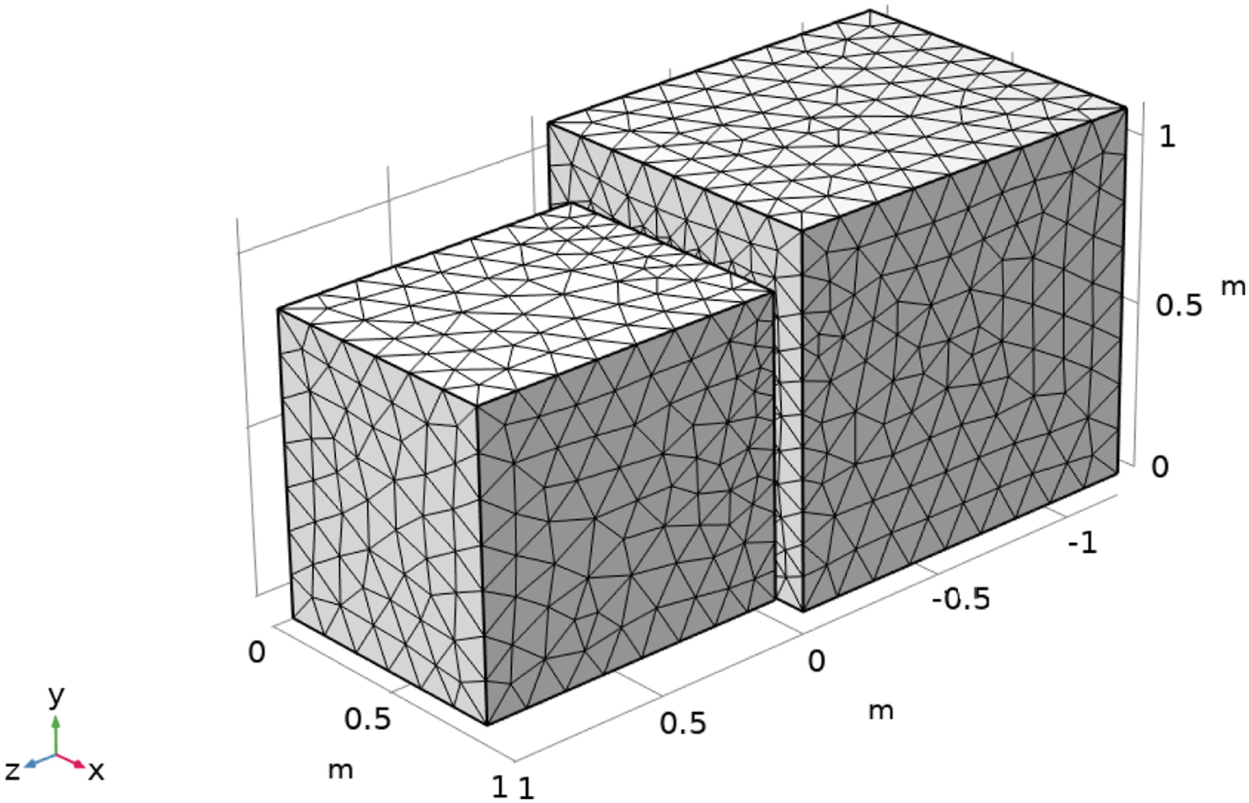

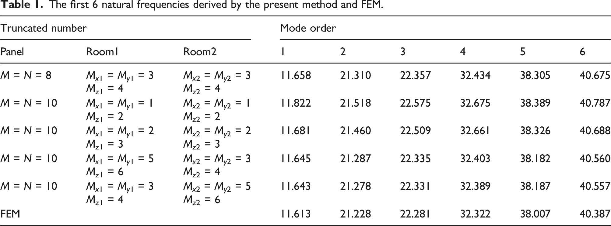
First, in order to verify the reliability and correctness of the model as shown in Figure 1, the first 6 natural frequencies under free condition and the sound pressure level in the sound source room and the receiving room under the action of a point source are calculated by the present method and the simulation software. The dimensions of the sound source room and receiving room are L_x1 × L_y1 × L_z1 = 3.0 m × 3.3 m × 3.6 m and L_x2 × L_y2 × L_z2 = 3.3 m × 3.6 m × 3.9 m. The limiting conditions in ISO 140 are simplified during analysis to save computing time and improve versatility. The medium in the acoustic cavity is air, and the parameters are sound velocity c₀ = 340 m/s, density ρ₀ = 1.21 kg/m³. The impedance of the receiving room is Z = (80-j)ρ₀c₀. The panel is elastically installed at the boundary of the two cavities through myriad linear springs and rotational springs, as shown in Figure 1(b). The dimensions of the partition are a × b × h = 2.5 m × 2.6 m × 0.008 m, the coordinates of the panel center in the sound source room and the receiving room are (1.5 m, 1.65 m, 3.6 m) and (1.65 m, 1.65 m, 0 m). The material parameters of the panel are mass density ρ = 2700 kg/m³, Young’s modulus E = 71 GPa and Poisson ratio v = 0.3. The stiffness of the linear springs and rotational springs on four sides are set as 10¹⁰ N/m and 10¹⁰ Nm/rad, so as to achieve the clamped support. When calculating the sound pressure level, the dimensions of the sound source room and receiving room are L_x1 × L_y1 × L_z1 = 0.8 m × 0.9 m × 1.0 m and L_x2 × L_y2 × L_z2 = 1 m × 1.1 m × 1.2 m. The dimensions of the partition are a × b × h = 0.5 m × 0.6 m × 0.008 m, the coordinates of the panel center in the sound source room and the receiving room are (0.4 m, 0.45 m, 1.0 m) and (0.5 m, 0.45 m, 0 m). Other parameters are the same as those for calculating the natural frequencies. The point sound source is located at (0.2 m, 0.2 m, 0.2 m) in the sound source room, and the amplitude of the source is Q_s = 2 × 10⁻⁶ m³/s. The response at point (0.4 m, 0.45 m, 0.5 m) inside the sound source room and point (0.3 m, 0.3 m, 0.3 m) inside the receiving room are derived. When determining the truncation coefficients, it must be ensured that c₀/F_up × M_i > L_i (i = x, y, z) to ensure the convergence of the result. Therefore, the truncation coefficients are set as M × N = 10 × 12, M_x1 × M_y1 × M_z1 = 5 × 5 × 6 and M_x2 × M_y2 × M_z2 = 5 × 6 × 7 during the calculation.

The natural frequencies of the sound insulation measurement model calculated by the present method and finite element method (FEM) are listed in Table 1. It is clearly that when the method proposed in this paper is used to calculate the cavity-panel-cavity model, the results of the natural frequencies under free condition are in good agreement with those of FEM under different truncation numbers. The results of sound pressure level in the sound source room and the receiving room are shown in Figure 3. It is obviously that the curves of sound pressure level inside the two rooms derived by the different methods agree very well.

Table 1.

The first 6 natural frequencies derived by the present method and FEM.

Truncated number			Mode order
Panel	Room1	Room2	1	2	3	4	5	6
M = N = 8	M_x1 = M_y1 = 3	M_x2 = M_y2 = 3	11.658	21.310	22.357	32.434	38.305	40.675
M = N = 8	M_z1 = 4	M_z2 = 4	11.658	21.310	22.357	32.434	38.305	40.675
M = N = 10	M_x1 = M_y1 = 1	M_x2 = M_y2 = 1	11.822	21.518	22.575	32.675	38.389	40.787
M = N = 10	M_z1 = 2	M_z2 = 2	11.822	21.518	22.575	32.675	38.389	40.787
M = N = 10	M_x1 = M_y1 = 2	M_x2 = M_y2 = 2	11.681	21.460	22.509	32.661	38.326	40.688
M = N = 10	M_z1 = 3	M_z2 = 3	11.681	21.460	22.509	32.661	38.326	40.688
M = N = 10	M_x1 = M_y1 = 5	M_x2 = M_y2 = 3	11.645	21.287	22.335	32.403	38.182	40.560
M = N = 10	M_z1 = 6	M_z2 = 4	11.645	21.287	22.335	32.403	38.182	40.560
M = N = 10	M_x1 = M_y1 = 3	M_x2 = M_y2 = 5	11.643	21.278	22.331	32.389	38.187	40.557
M = N = 10	M_z1 = 4	M_z2 = 6	11.643	21.278	22.331	32.389	38.187	40.557
FEM			11.613	21.228	22.281	32.322	38.007	40.387

Figure 3.

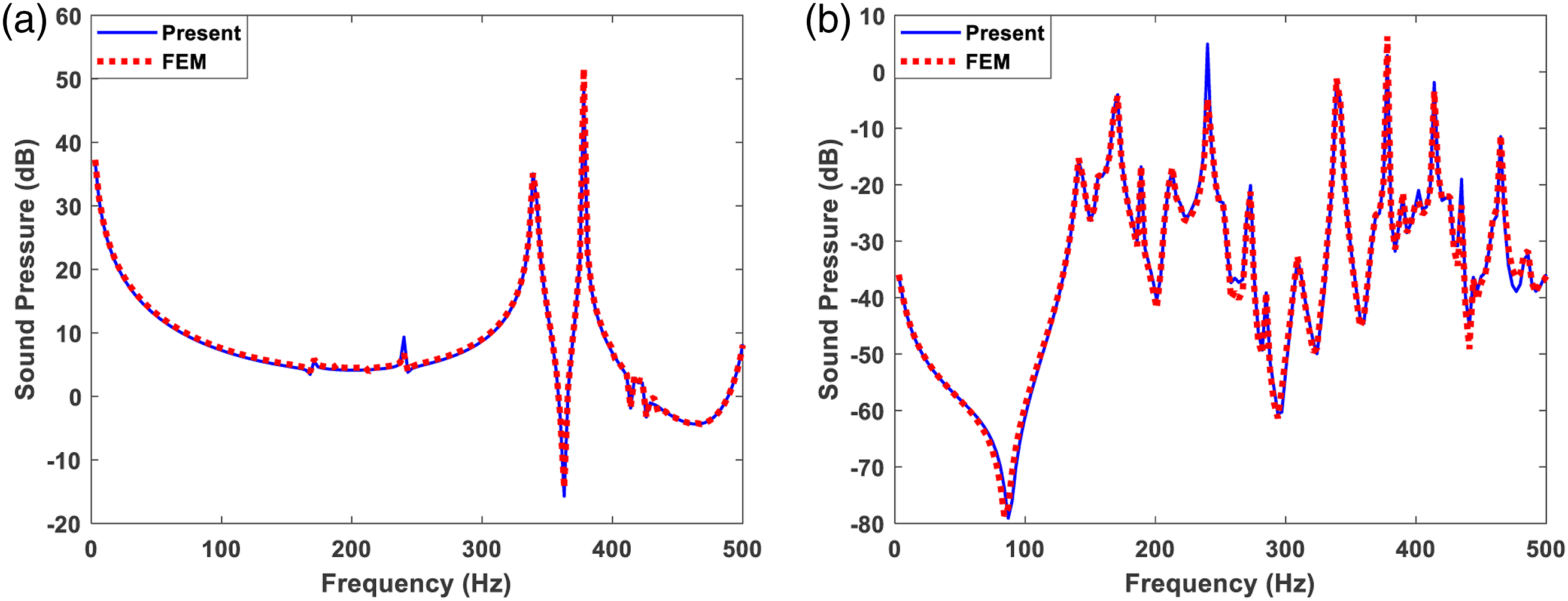
Sound pressure level obtained by the present method and FEM. (a) Sound source room. (b) Receiving room.

Next, the STL is calculated according to the sound pressure method and the result was compared with that in the Reference 22 to study the sound insulation characteristics of the panel structures. The results are shown in Figure 4. It can be noticed from the figure that the trends of the two curves are basically the same, but there are still some differences. The main reason is that the calculation method in this paper is different from that in the reference. The mean square sound pressure average of the test points is linked to the acoustic potential energy of the two rooms, but the sound pressure level of the room in this paper is directly calculated by equation (35). Besides, the different impedance boundary of the rooms and the damping coefficients of the panel and air assumed will also contribute to this phenomenon. It can be found that STL is greatly affected by the environmental factors and there is no accurate method to measure this acoustic quantity, so a certain difference is acceptable.

Figure 4.

Sound transmission loss obtained by the present method and the reference.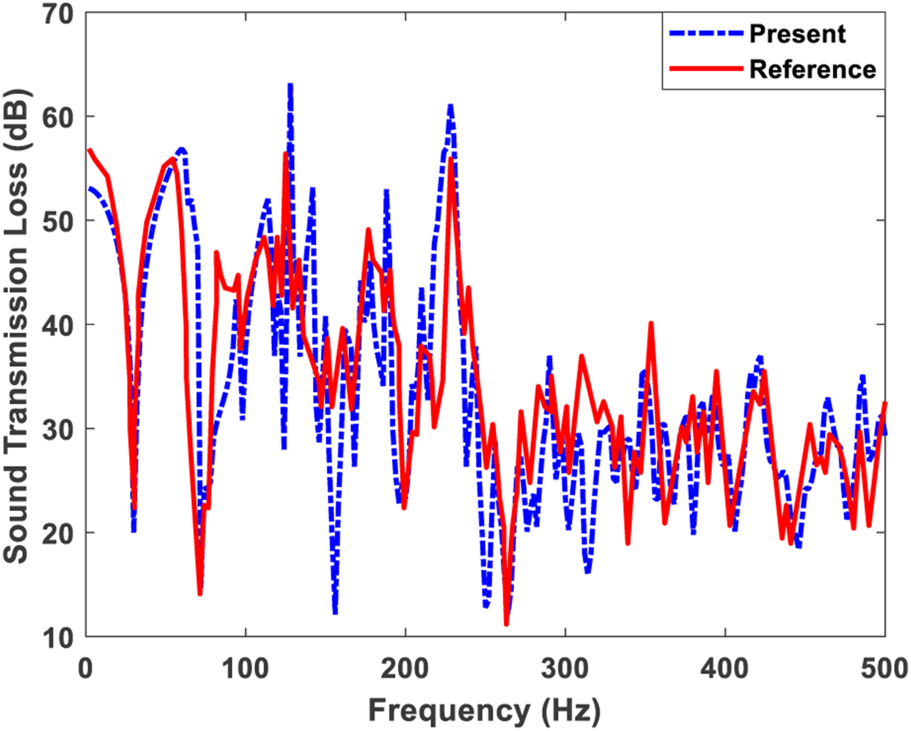

Relationship between impedance and reverberation time T₆₀

Two virtual experiments are carried out to study the relationship between the impedance of a rectangular cavity and its reverberation time T_60. In the investigation of the position of the absorbing wall, the dimensions of the rectangular cavity are L_x × L_y × L_z = 1.0 m × 1.3 m × 1.6 m. The medium in the acoustic cavity is air, and the parameters are sound velocity c₀ = 340 m/s, density ρ₀ = 1.21 kg/m³. In the investigation of the number of the absorbing walls, the dimensions of the rectangular cavity are L_x × L_y × L_z = 1.5 m × 1.5 m × 1.5 m to avoid the influence of different areas on the results. The impedance of the boundary is set as Z = 300 × (50-j) in the two cases. The truncation coefficients of the cavity are M_x × M_y × M_z = 5 × 5 × 6 during the calculations.

From Figure 5(a), there are only two kinds of reverberation times at the first 30 modes when there is only one sound-absorbing wall. Moreover, the same reverberation time will decline with the increase of the area of sound-absorption wall (S_z0 = 1.0 × 1.3 m², S_y0 = 1.0 × 1.6 m², S_x0 = 1.3 × 1.6 m², S_z0 is the area of the face z = 0 or L_z, the other representations are the same). As shown in Figure 5(b), the value of the reverberation time begins to increase when the number of sound-absorbing walls is greater than two. It could also be observed that the more the sound-absorbing walls are, the smaller the reverberation time is. And this law is applicable to each mode.

Figure 5.

Effect of the sound-absorbing walls on the reverberation time T_60. (a) One sound-absorbing wall at different positions. (b) Different numbers of absorbing walls.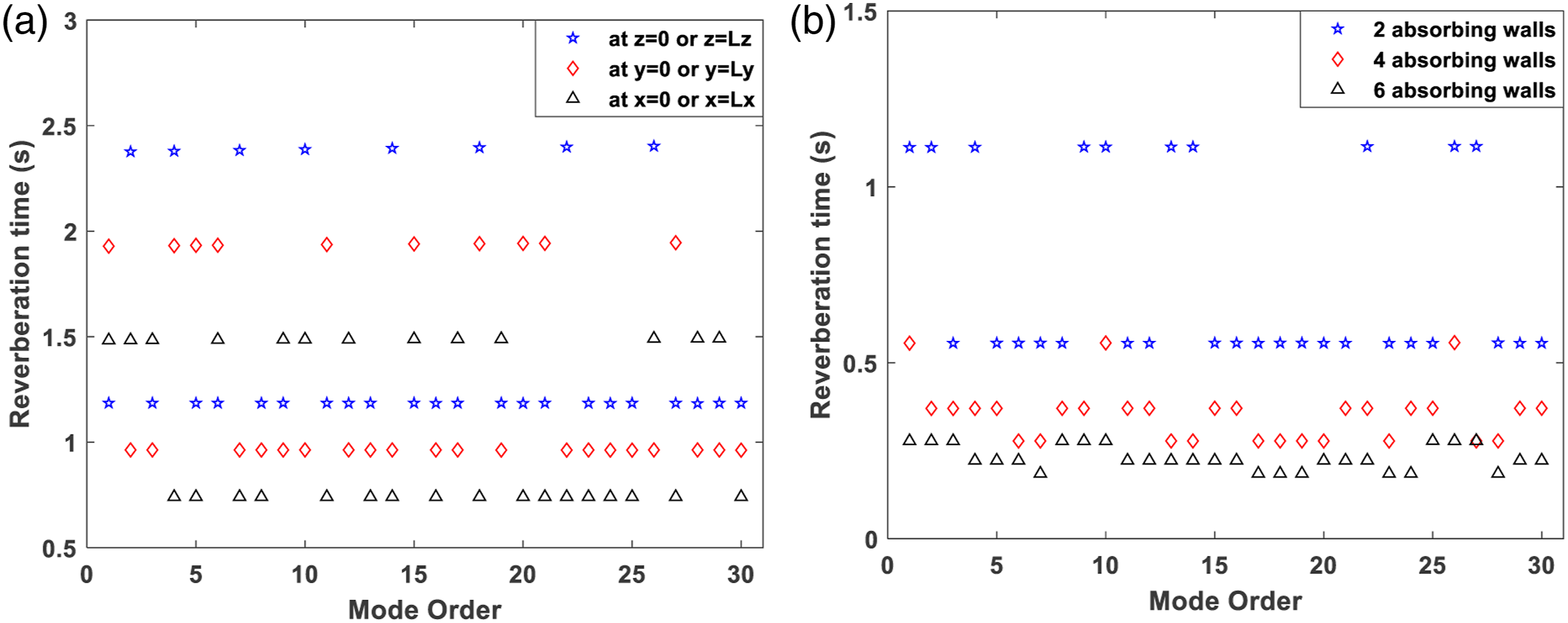

Effect of thickness under different boundary conditions

In this part, the influence of the thickness on the STL are investigated. The thickness of the panel h is selected as 0.003 m, 0.006 m, 0.009 m, or 0.012 m. The dimensions of the source room and the receiving room are selected as L_x1 × L_y1 × L_z1 = 1.3 m × 1.5 m × 1.7 m and L_x2 × L_y2 × L_z2 = 1.4 m × 1.6 m × 1.8 m. The medium in the acoustic rooms is air, and the parameters are sound velocity c₀ = 340 m/s, density ρ₀ = 1.21 kg/m³. The impedance of the receiving room is Z = (80-j)ρ₀c₀. The width and length of the panel are a × b = 0.6 m × 0.7 m and the coordinates of the center of the panel in the sound source room and receiving room are (0.65 m, 0.75 m, 1.7 m) and (0.7 m, 0.75 m, 0 m). The material parameters of the panel are mass density ρ = 2700 kg/m³, Young’s modulus E = 71 GPa, and Poisson ratio v = 0.3. Clamped support, mixed support, and simple support are used for the installation, so the stiffness of the linear springs is k = 10¹⁰ N/m and that of the rotational springs is K = 0 Nm/rad or 10¹⁰ Nm/rad. The point sound source is located at (L_x1/2, L_y1/2, L_z1/2) in the source room, and the amplitude is Q_s = 2 × 10⁻⁶ m³/s. The simulation frequency range is chosen as 0–2239 Hz to meet the need of virtual experiments (Excessive calculation frequency will consume a lot of time). Considering the size of the model and the frequency range, the truncation numbers of the panel are set as M × N = 10 × 11; Those of the two cavities are chosen as M_x1 × M_y1 × M_z1 = 11 × 11 × 12 and M_x2 × M_y2 × M_z2 = 11 × 11 × 12 during the calculation. Randomly selecting 18 measuring points in the sound source room, the STL is computed by the sound pressure method. Figure 6 are the STL with different thickness under different boundary conditions ranging from 0 to 2239 Hz. Figure 7 are the results of the third octave band and the maximum center frequency is 2000 Hz.

Figure 6.

Sound transmission loss of different thickness under different boundary conditions. (a) CCCC. (b) SSSS. (c) CSCS. (d) CSSS.

Figure 7.

Results of the sound transmission loss of different thickness under different boundary conditions in the form of third octave band. (a) CCCC. (b) SSSS. (c) CSCS. (d) CSSS.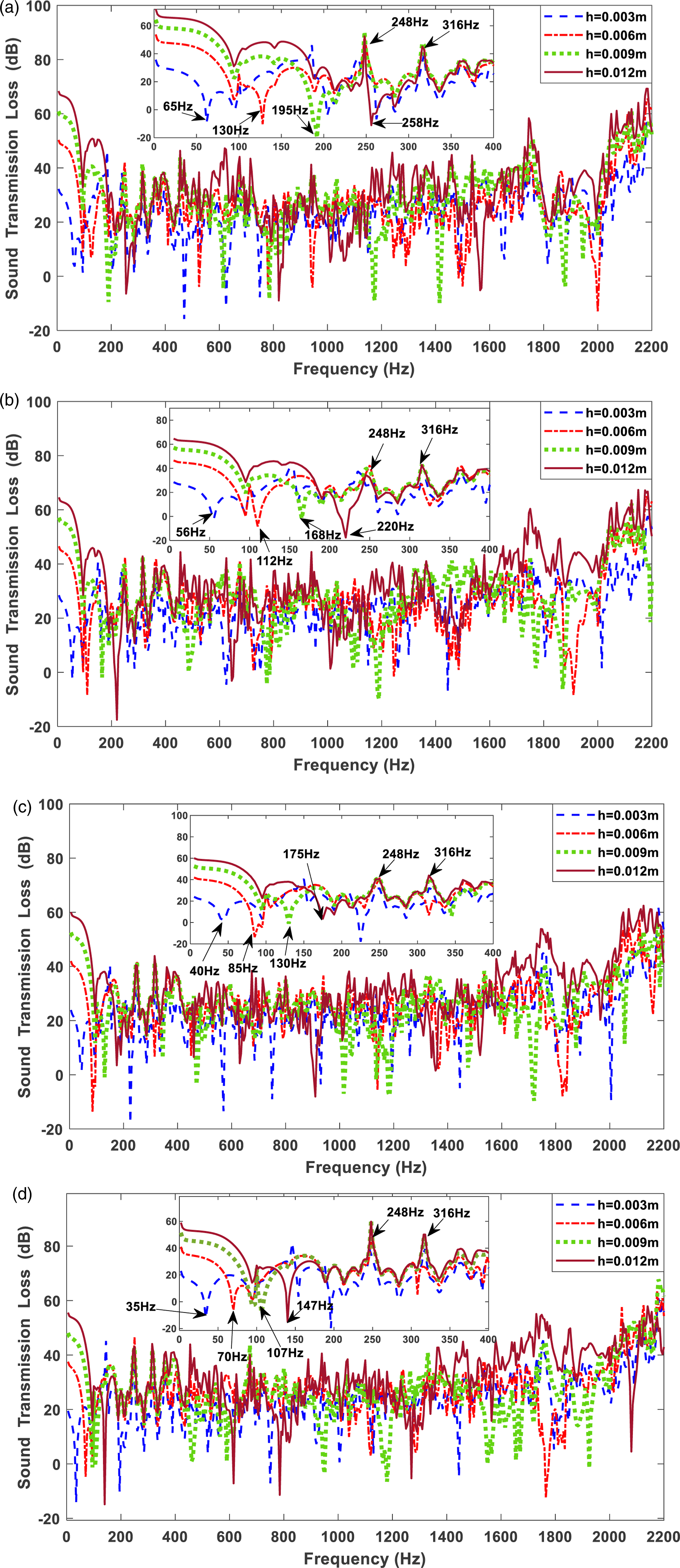

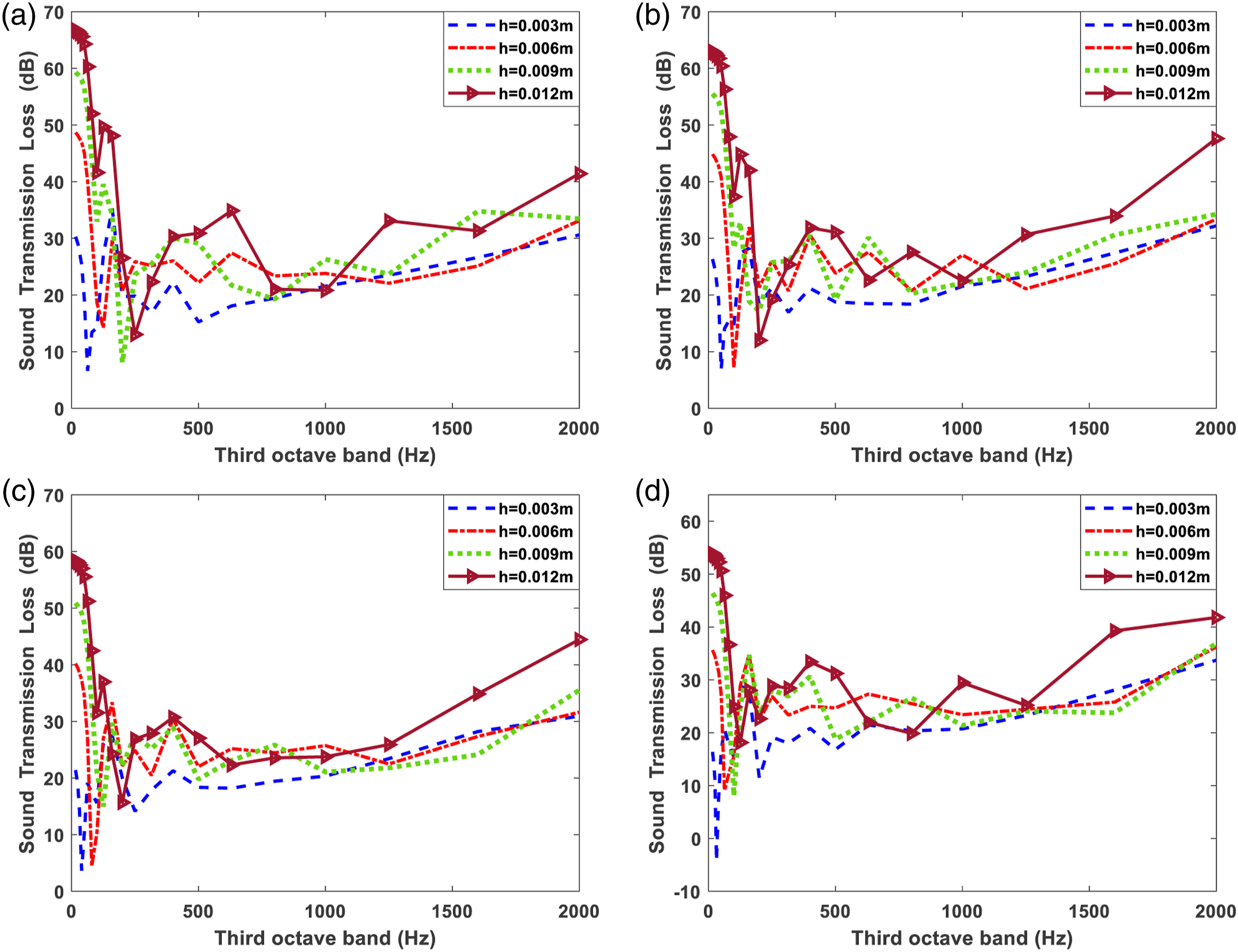
It could be figured out from Figure 6 that the thickness of the panel has a significant impact on the sound insulation characteristics of the model. Figure 7 shows that the curves have a common trend that they fluctuate violently before 300 Hz and then rise slowly. This phenomenon can be mainly concluded that the thickness and the modes of the components have a great effect on the STL in the low-frequency band. The effect of natural modes is reduced due to the increase of nodes. The thicker the panel is, the better the sound insulation will perform. In addition, there is hardly difference among three curves in high-frequency domain except the thickest one. Also, the boundary conditions are changed in Figure 7, which can be seen that the STL is inversely proportional to the number of simple supports. As marked in the figures, 130 Hz, 195 Hz, 258 Hz in Figure 5(a); 56 Hz, 112 Hz, 168 Hz, 220 Hz in Figure 5(b); 40 Hz, 85 Hz, 130 Hz, 175 Hz in Figure 5(c); 35 Hz, 70 Hz, 107 Hz, 147 Hz in Figure 5(d), these are all the first natural frequencies of the panel under the four different thickness and it is interesting that they all appear in the form of troughs on the curves. This phenomenon can be mainly explained that when the plate structure resonates, the vibration amplitude of the plate increases, resulting in the increase of radiated sound power, so the sound insulation performance will be greatly weakened. Besides, the main anti resonance peaks show a trend of moving to the left with the number of simply supported boundaries increasing.

In order to further study the sound insulation characteristics in low-frequency band, Figure 6(a)–(c) also give out the results from 0 to 400 Hz in frequency domain. It is worth noting that the curves appear a coincident peak at 248 Hz and 316 Hz regardless of the thickness. This is induced by the 16th and the 27th modes of the receiving room. Therefore, it also has nothing to do with the boundary condition. To observe the vibration of the panel clearly in the resonance region, the velocity on the surface of the panel (h = 0.003 m) at 228 Hz are given in Figure 8. It is obvious that the vibration will intensify with the increase of the number of simple supports.

Figure 8.

Velocity on the surface of the panel (h = 0.003 m) at 248 Hz under different boundary conditions. (a) CCCC. (b) SSSS. (c) CSCS. (d) CSSS.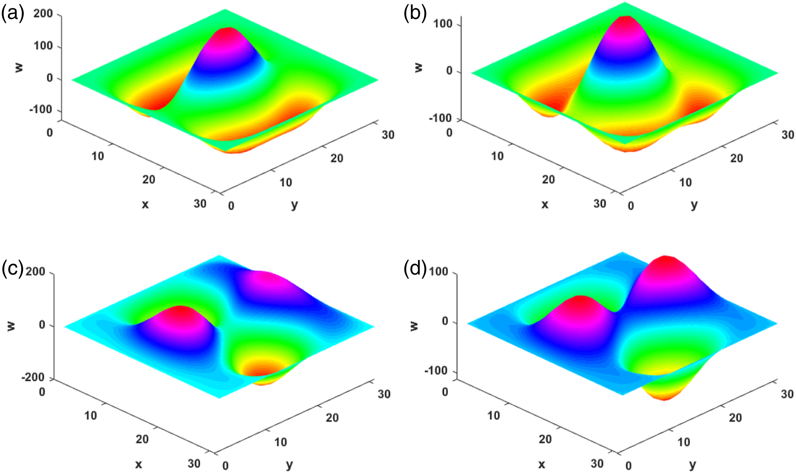

In summary, the thicker panel has greater influence on the sound insulation performance of the plate whereas this law seems does not apply in a specific frequency band due to the effect of the acoustic modes. Also, the coupling effect between the cavities and the panel is more remarkable when the panel is thicker. With the modes of rooms appearing, the sound insulation capacity of the panel will be significantly improved. This is mainly due to the emergence of room modes, which weakens the vibration of the structure at the corresponding frequency and makes it difficult to vibrate violently. Therefore, the radiated sound power is weak, while the incident sound power remains unchanged.

Effect of cavity length under different boundary conditions

In order to understand more extreme cases, the influence of the length of the receiving room is studied in this part. The dimensions L_x2 × L_y2 = 1.4 m × 1.6 m of the receiving room are kept unchanged to control the number of the variables. In this simulation experiment, the length of the receiving room L_z2 is selected as 0.1 m, 0.6 m, 1.8 m, or 3.6 m to change the length of the receiving room. When L_z2 = 3.6 m, to achieve enough normal modes, the truncation number M_z2 has to be over 20 to guarantee c₀/F_up × M_z2 > L_z2. The dimensions of the panel are a × b × h = 0.5 m × 0.6 m × 0.008 m. Clamped support is used for the installation, so the stiffness of the linear springs is k = 10¹⁰ N/m and the stiffness of the rotational springs is K = 10¹⁰ Nm/rad. At the same time, the calculation is also carried out under two different conditions that when the wall z = L_z2 of the receiving room is rigid, the impedance is Z = 5j × 10¹⁰. When the wall z = L_z2 is a pressure release surface, the impedance is Z = 1j × 10⁻⁵. The other parameters of the model are kept the same as those in Effect of thickness under different boundary conditions.

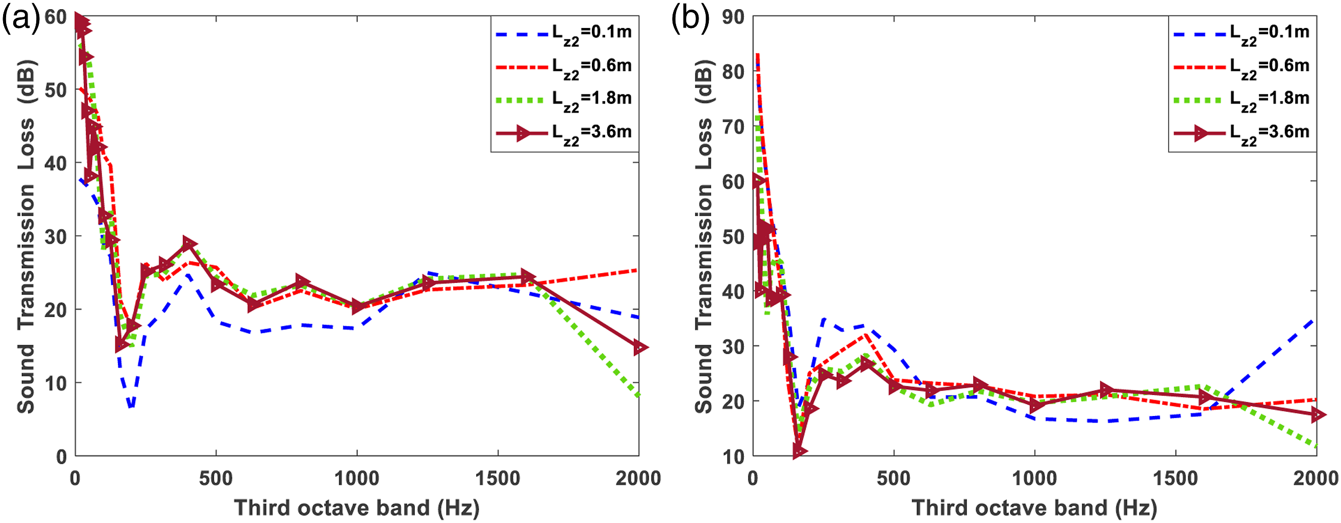
The degree of sound insulation between the subsystems involved in the problem has been analyzed. As shown in Figure 9, the STL is in good agreement with different length of the receiving room before 1800 Hz. From the whole frequency, it seems like the curve of 0.6 m has the best stability among the results. Moreover, the curve of L_z2 = 0.1 m is quite different from the other three curves, the STL is significantly lower than the other three cases. The length of the sound cavity has a relatively small impact on the sound insulation performance of the panel. It is apparent that the plate is not vulnerable to external influence due to its own characteristics. When the length of the room changes, the sound field in the room changes accordingly, but the STL is mainly related to the physical properties of the structure itself. The results of frequency domain ranging from 1800 Hz to 2200 Hz are also given in Figure 9, the curve of 1.8 m decreased significantly due to two valley values (2031 Hz and 2137 Hz) with large amplitude. After calculation, it can be confirmed that 2031 Hz is the normal mode of the panel and 2137 Hz is the normal mode of the receiving room. Due to the coupling relationship, such peaks do not appear on all curves. As the volume of the receiving room increases, the curve of the STL fluctuates more violently in the low frequency range. This situation is caused by the enlargement of the size, which leads to the concentration of the natural frequencies in the low-frequency band. It can be seen that with the addition of plate modes, the sound insulation will be significantly reduced. This is mainly because the vibration of the structure at the corresponding frequency is enhanced due to the emergence of modes, which leads to the strengthening of radiated sound power, while the incoming sound power remains unchanged, and the STL will be reduced accordingly. (Figure 10).

Figure 9.

Sound transmission loss of different length under two boundary conditions. (a) Wall z = L_z2 is a rigid surface. (b) Wall z = L_z2 is a pressure relief surface.

Figure 10.

Results of the sound transmission loss of different length under two boundary conditions in the form of third octave band. (a) Wall z = L_z2 is a rigid surface. (b) Wall z = L_z2 is a pressure relief surface.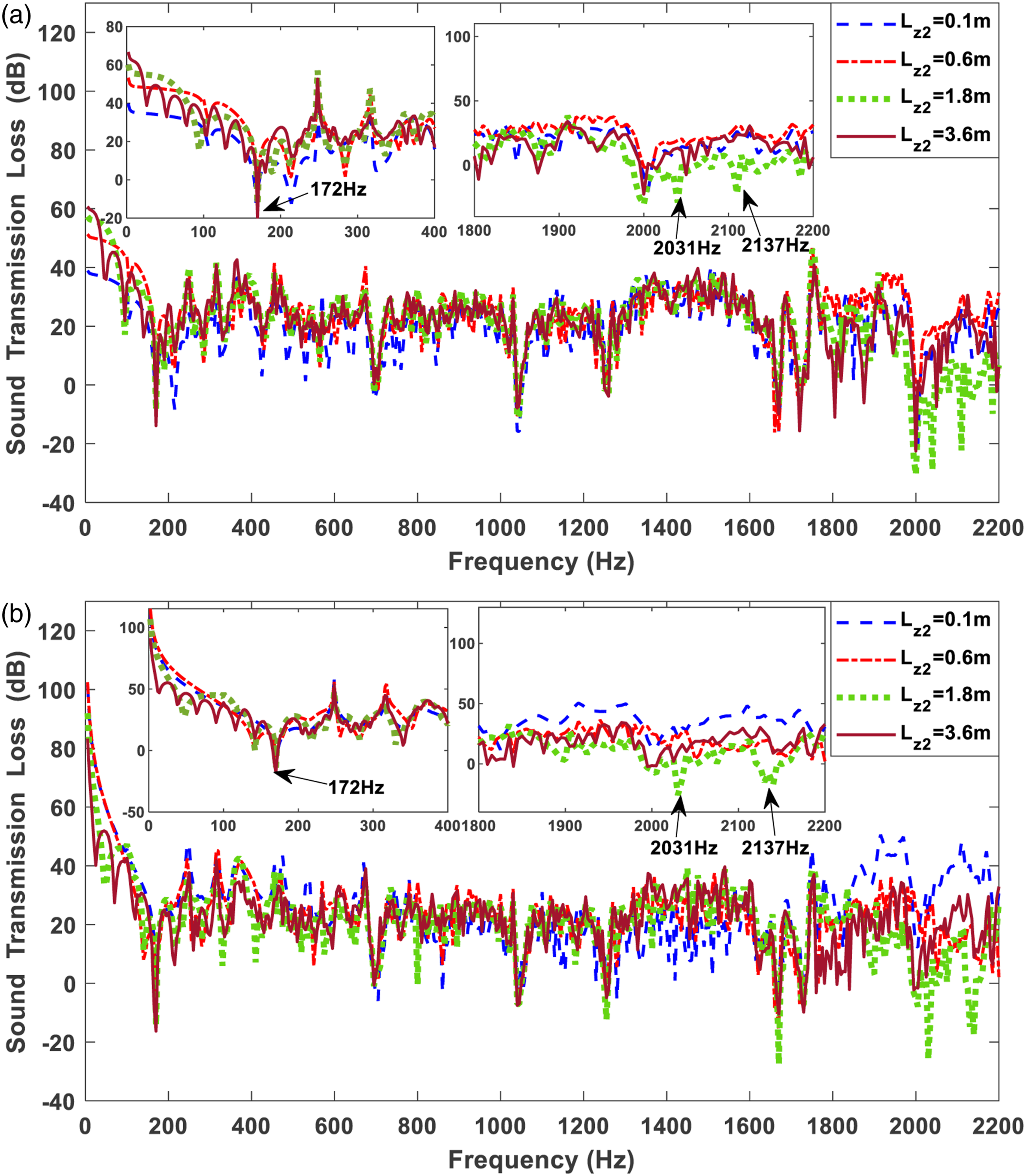

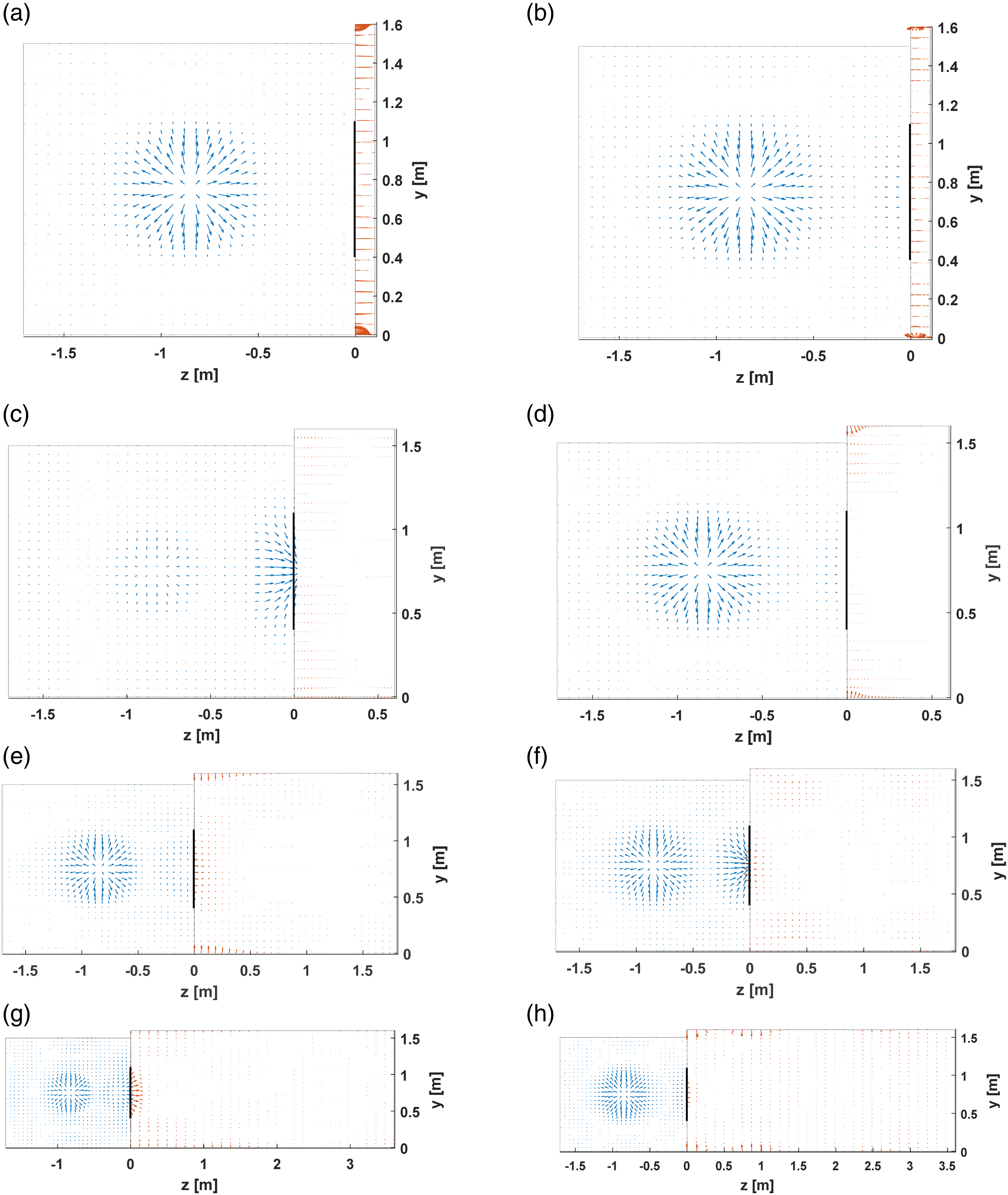
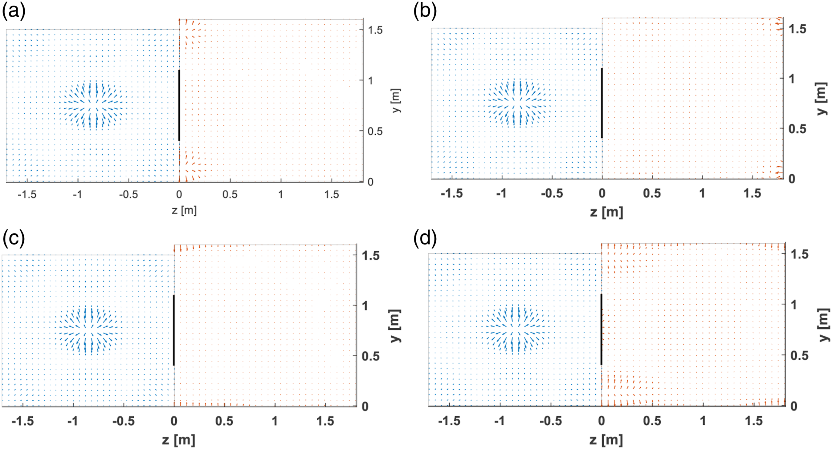
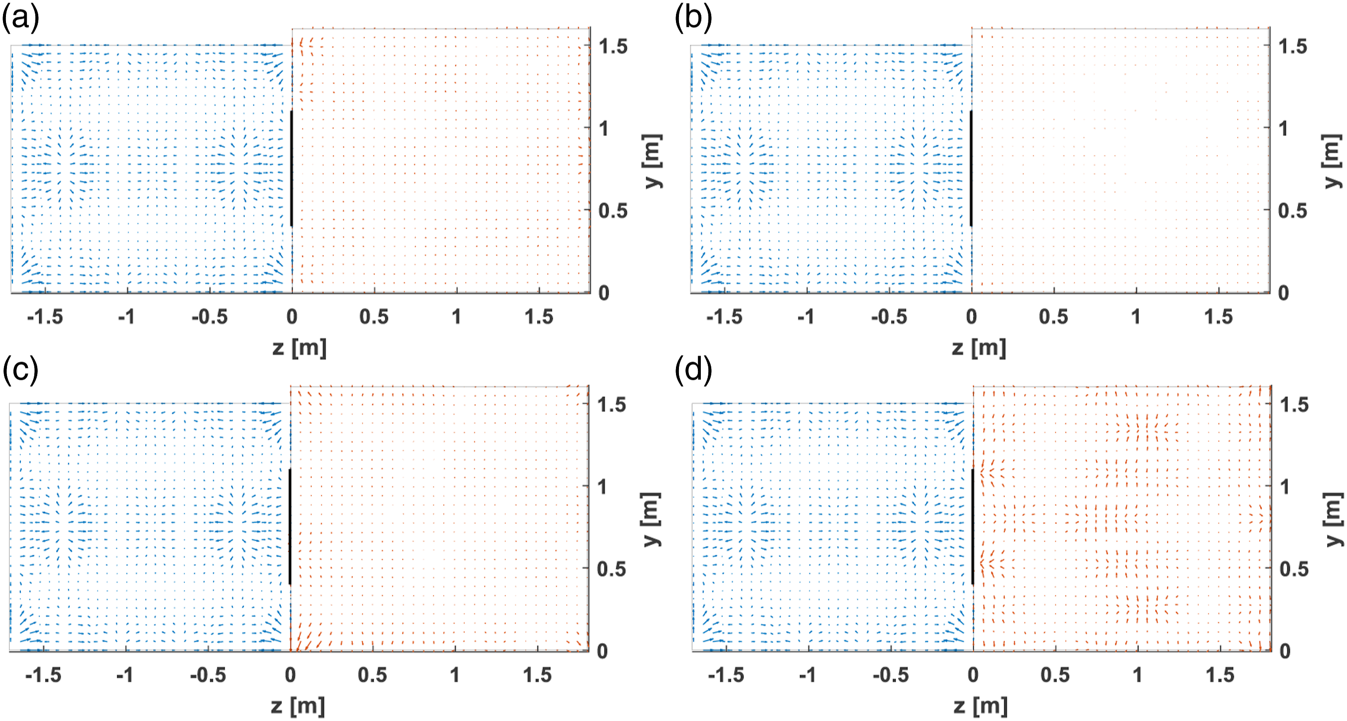
At 172 Hz, the four curves all have a downward coincident peak and this is mainly caused by the natural mode of the panel. To better understand the sound field inside the suite, Figure 11 and Figure 12 are the sound pressure distribution drawings at 172 Hz, from which it can be known that boundary conditions greatly affect the sound pressure distribution inside the rooms. Figure 13 is the images in Y-Z plane when x = L_x1/2, which is intercepted for analysis of sound intensity. It can be noticed that the power radiates around the sound source and the intensity inside the system is uniformly distributed. There is a sound intensity concentration at the surface coupled with the panel, and this phenomenon is most remarkable when the receiving room appears as a long strip. The practical results also show that in comparison with the rigid boundary condition, the free one is a better way to solve the energy concentration at the normal modes of the system.

Figure 11.

When wall z = L_z2 is a rigid surface, the sound pressure distribution inside the suite at 172 Hz. (a) L_z2 = 0.1 m. (b) L_z2 = 0.6 m. (c) L_z2 = 1.8 m. (d) L_z2 = 3.6 m.

Figure 12.

When wall z = L_z2 is a pressure relief surface, the sound pressure distribution inside the suite at 172 Hz. (a) L_z2 = 0.1 m. (b) L_z2 = 0.6 m. (c) L_z2 = 1.8 m. (d) L_z2 = 3.6 m.

Figure 13.

Sound intensity distribution inside the suite at 172 Hz. The left side represents wall z = L_z2 is a rigid surface, the right side represents wall z = L_z2 is a pressure relief surface. (a), (b) is L_z2 = 0.1 m. (c), (d) is L_z2 = 0.6 m. (e), (f) is L_z2 = 1.8 m. (g), (h) is L_z2 = 3.6 m.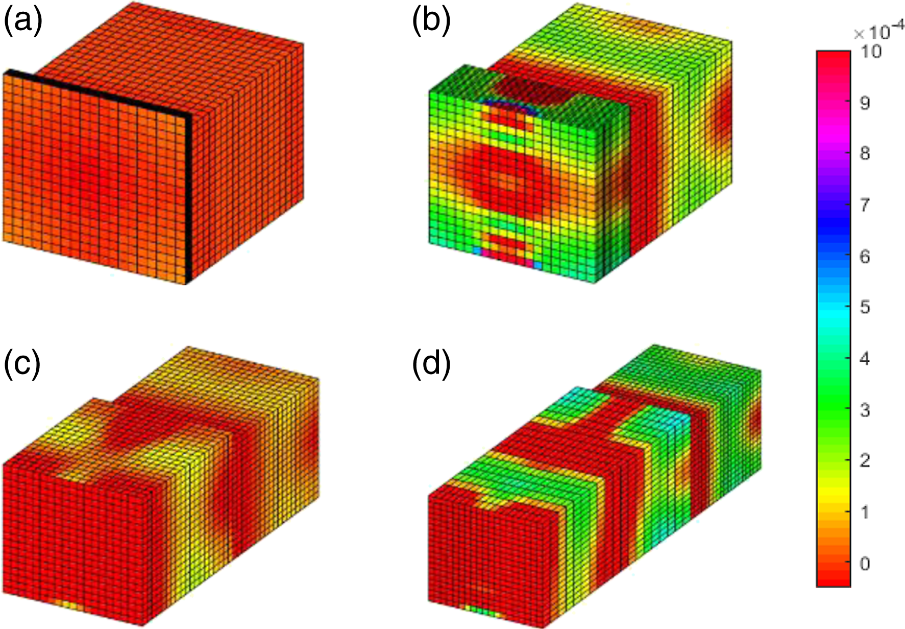

Effect of impedance boundary of receiving room

In this section, examples are presented to illustrate how the impedance boundary affect the transmission of sound based on the virtual model. In the cases of weak impedance and gradient impedance, the effect of the impedance on the STL, the sound pressure distribution and the sound intensity field inside the model are observed. During the calculation, the main boundary parameters are listed in Table 2. Other parameters of the model are kept same as those in Effect of thickness under different boundary conditions.

Table 2.

The impedance boundary used in this section.

Type	Simulation order
Type	a	b	c	d
Gradient impedance	1j × 10	1j × 100	1j × 1000	1j × 10⁶
Weak impedance	1j × 10³	2j × 10³	3j × 10³	6j × 10³

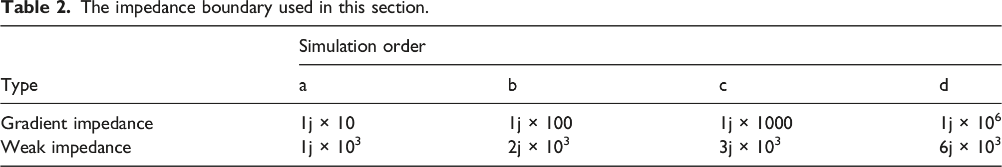
As shown in Figure 14(a), the curve of Z = 1j × 10⁶ is quite different from the others because it goes down sharply when the frequency is 1650 Hz. The same situation also occurs when Z = 6j × 10³ under the condition of weak impedance. It is surprised to find that the two curves have a common valley at 1995 Hz and it is neither the mode of the cavities nor the mode of the panel. Thus, it can only be caused by the superposition of coupling relationship under the excitation of sound source. Most notably, the increase of impedance will change the natural frequency of the system, which will make the sound insulation curve more complex. In the case of gradient impedance, the curves of Z = 1j × 100 and Z = 1j × 1000 show an upward trend due to the peak values whereas the curve of Z = 1j × 10 stays stable since the fluctuations in the opening stage. On the contrary, the other three curves both are stable at about 10–20 Hz in the case of weak impedance.

Figure 14.

Results of the sound transmission loss of different impedance boundary in the form of third octave band. (a) Gradient impedance. (b) Weak impedance.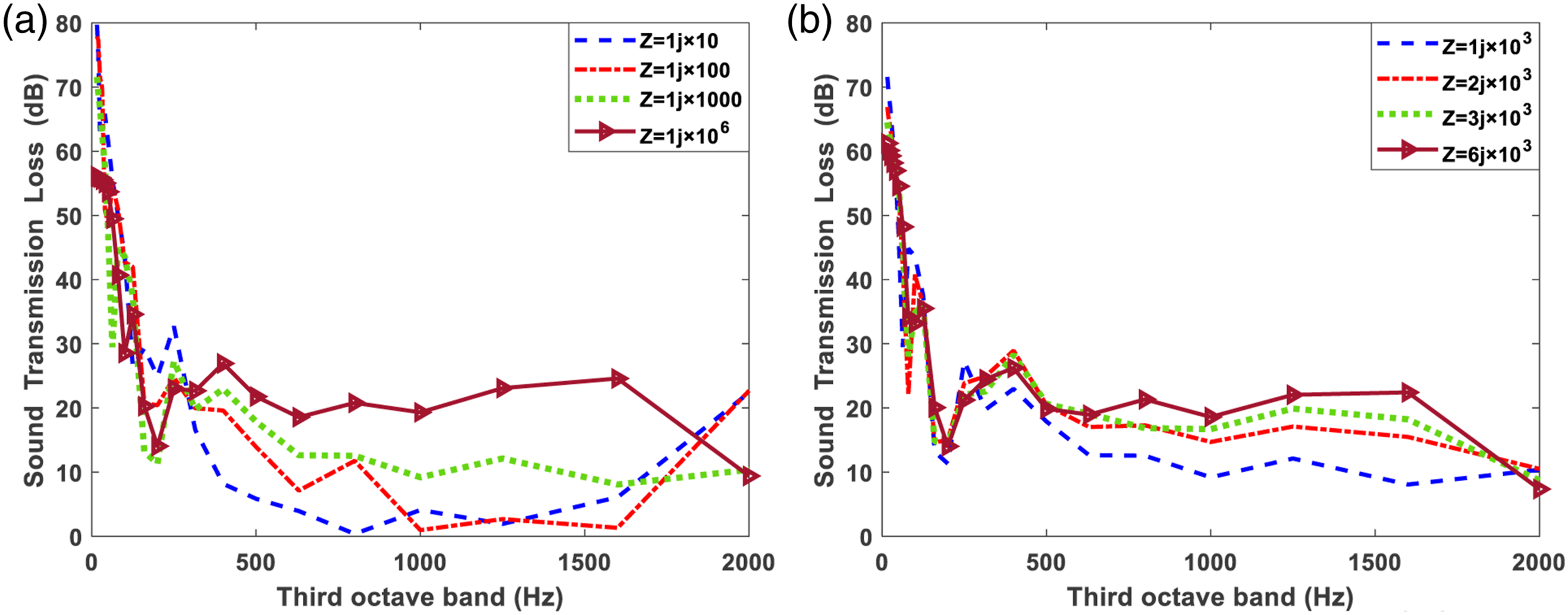

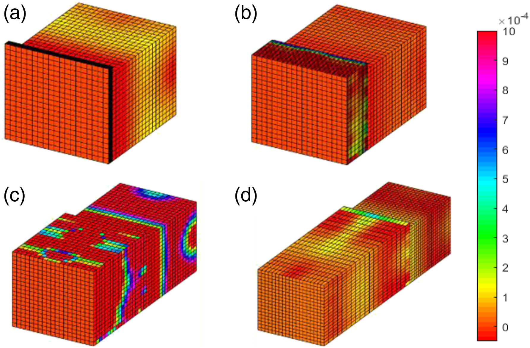
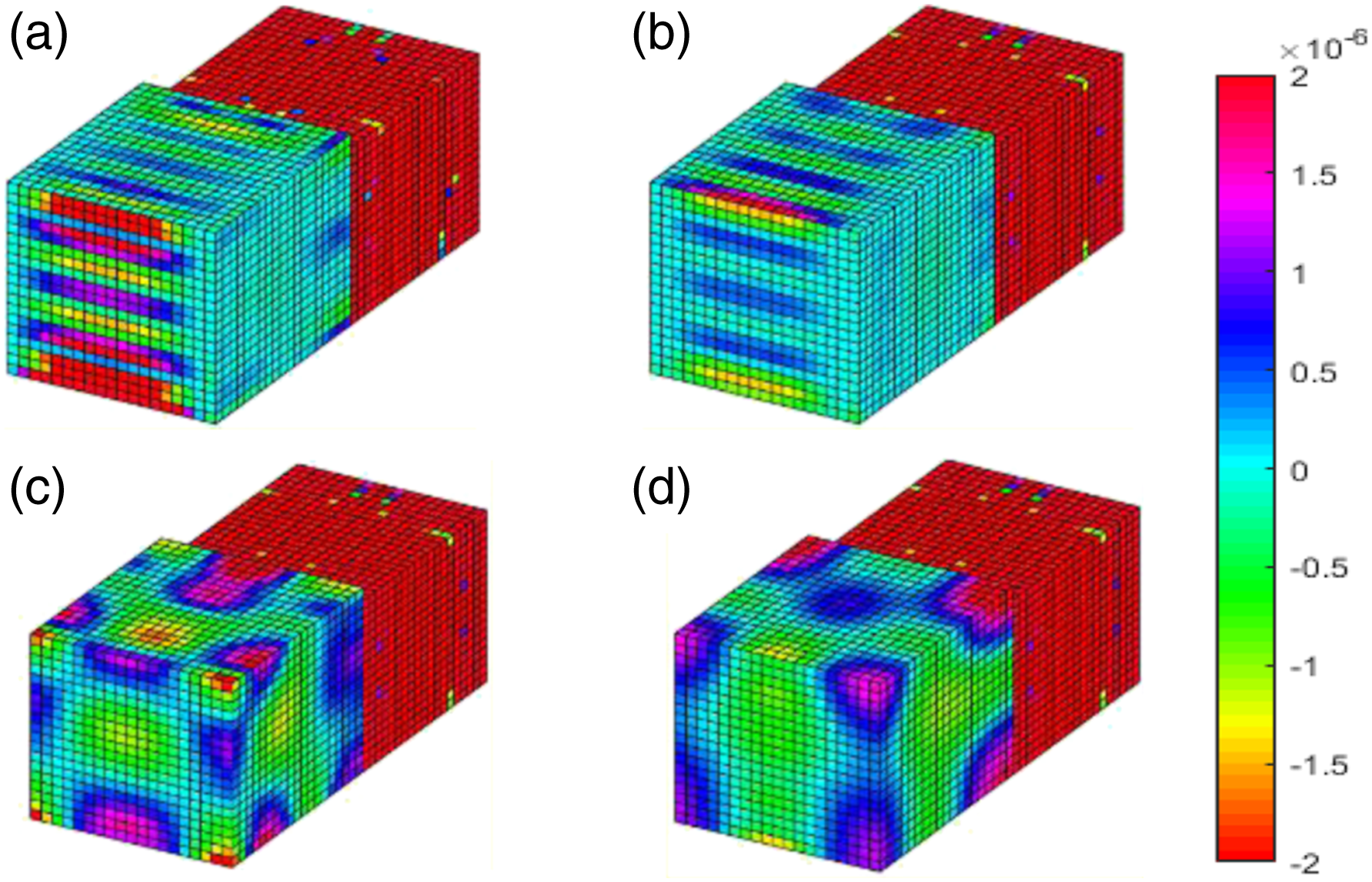
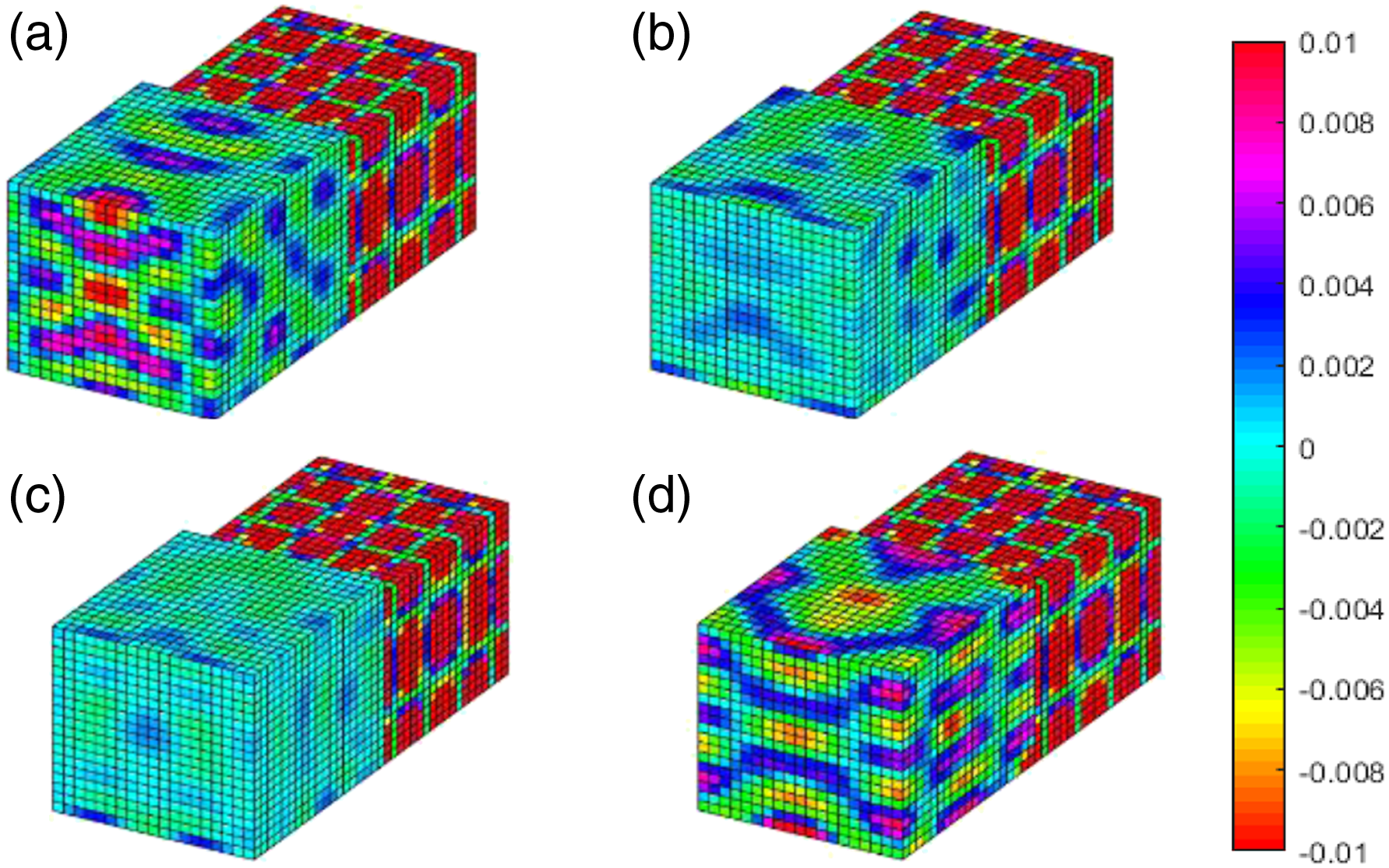
As marked in Figure 15, 245 Hz, 316 Hz, 675 Hz, and 695 Hz are all the normal modes of the cavities. To better understand the sound field inside the suite, Figure 16 and Figure 17 are the drawings of sound pressure distribution at 316 Hz and 695 Hz. The pressure is symmetrically distributed and the sound pressure in the receiving room increases with the enhancement of impedance. The increase of rigidity enhances the effect of sound wave reflection in the receiving room, resulting in the concentration of sound energy in the corners of the room. It could be observed the sound pressure in the sound source room keep at a high level in the case of gradient impedance. This phenomenon also corresponds to the situation that only the curve in this case has an obvious peak at this frequency in Figure 15. Figure 18 and Figure 19 are the sound intensity field inside the suite when x = L_x1/2 with different impedance at 316 Hz and 695 Hz. From the figures, it can be found that the sound intensity on the walls of the receiving room increases with the impedance rising as gradient whereas this phenomenon is not clear under weak impedance. It is also worth mentioning that the phenomenon that energy concentration is at the sound source no longer exists at 695 Hz. Instead, it changes to a pair of symmetrical divergence points.

Figure 15.

Sound transmission loss of different impedance boundary. (a) Gradient impedance. (b) Weak impedance.

Figure 16.

Sound pressure distribution inside the suite under gradient impedance at 316 Hz. (a) Z = 1j × 10. (b) Z = 1j × 100. (c) Z = 1j × 1000. (d) Z = 1j × 10⁶.

Figure 17.

Sound pressure distribution inside the suite under weak impedance at 695 Hz. (a) Z = 1j × 10³. (b) Z = 2j × 10³. (c) Z = 3j × 10³. (d) Z = 6j × 10³.

Figure 18.

Sound intensity distribution inside the suite under gradient impedance at 316 Hz. (a) Z = 1j × 10. (b) Z = 1j × 100. (c) Z = 1j × 1000. (d) Z = 1j × 10⁶.

Figure 19.

Sound intensity distribution inside the suite under weak impedance at 695 Hz. (a) Z = 1j × 10³. (b) Z = 2j × 10³. (c) Z = 3j × 10³. (d) Z = 6j × 10³.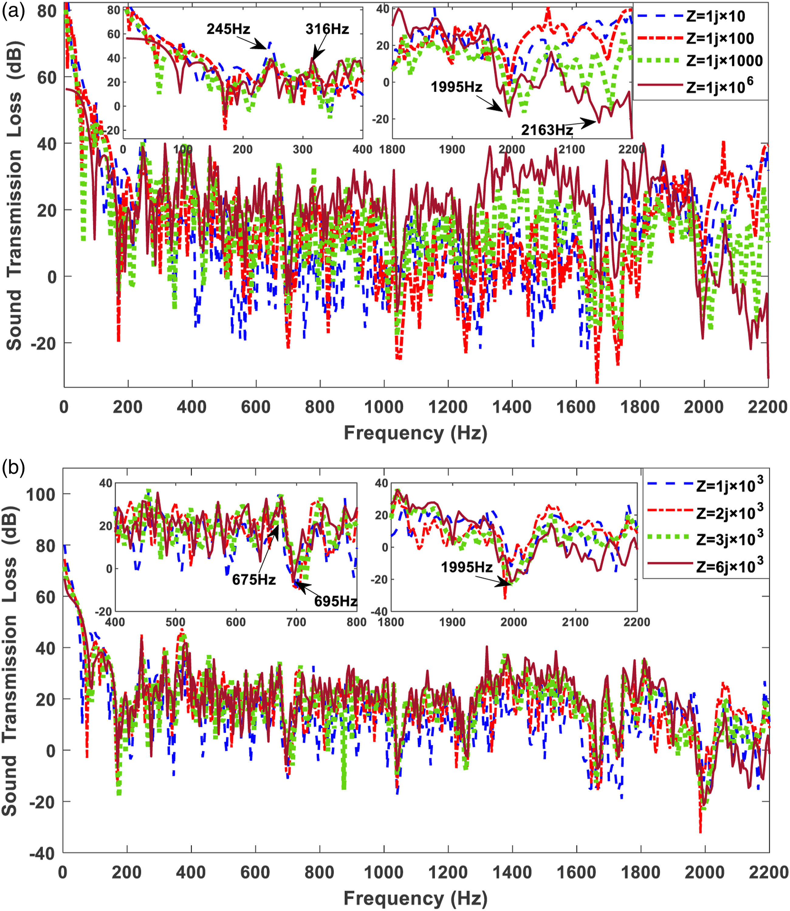

In general, the increase of the impedance of the sound absorption chamber leads to the change of the normal modes and the STL measured will decrease significantly in the high-frequency band when the receiving room reaches a state of approximate reverberation. Moreover, in the case of weak impedance, the curves of sound insulation tend to be stable after fluctuation ranging from 0 to 200 Hz and the STL changes little under different conditions while showing a downward trend, which may be because the sound energy distribution in the cavity is mainly controlled by a few low-order sound modes in low-frequency band. At the same time, the sound energy density and the incident sound pressure on the plate stay unchanged, and then the sound radiation power of the panel remain basically stable.

Effect of medium parameters

The sound velocity under different temperature and relative humidity are given in Figure 20. From Figure 20(a), it is clearly that the change of relative humidity at the same temperature has little effect on the sound velocity. Only when the temperature is very high, such like 90°C, the sound velocity is going to change greatly with the increase of relative humidity. Obvious law has been found in Figure 20(b) that the speed of sound will showing a sharp upward trend with temperature rising under the same humidity and the curves with bigger humidity will have greater slope when it is over 20°C. Since the relative humidity has little influence on the sound velocity in the air, the temperature is taken as the main factor affecting the sound velocity and the influence of the environmental relative humidity will be ignored in the follow-up work.

Figure 20.

Sound velocity affected by medium parameters. (a) Temperature. (b) Relative humidity.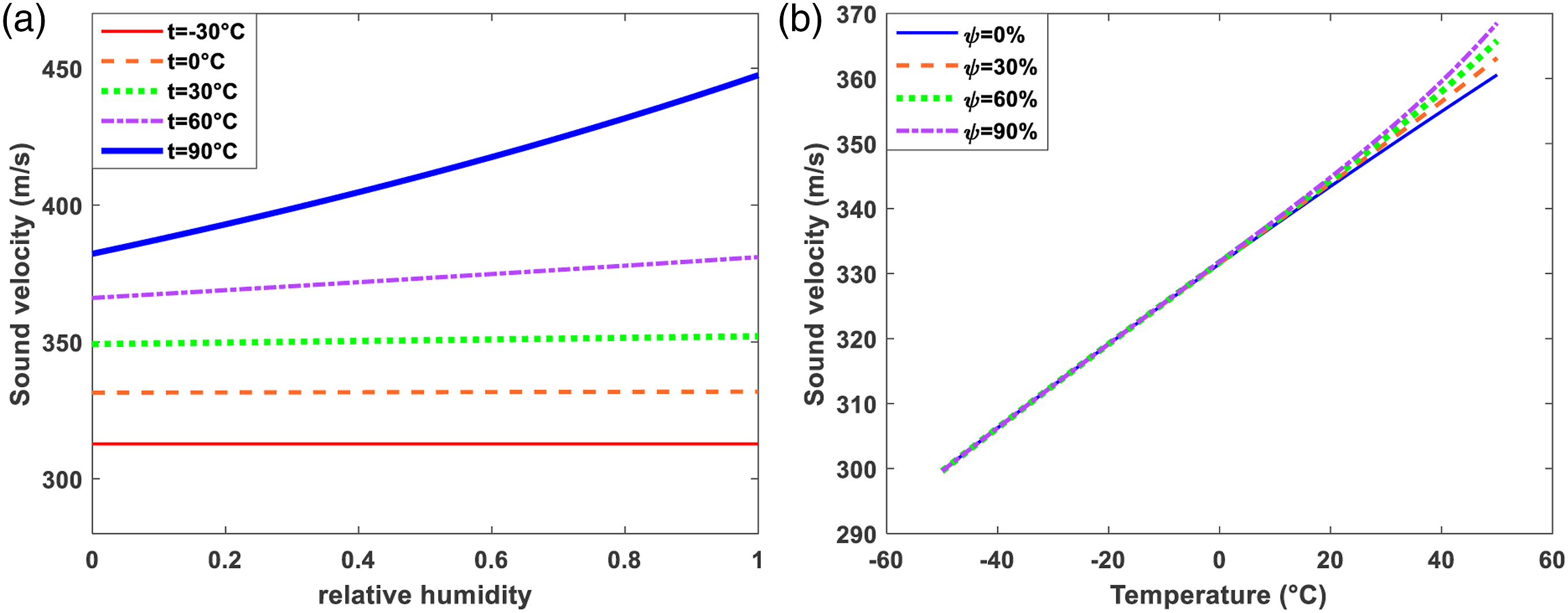

To further explore the relationship between acoustic characteristics and temperature and relative humidity, a standard bigger acoustic measurement suite is applied in this part. The dimensions of the source room and the receiving room are L_x1 × L_y1 × L_z1 = 2.07 m × 2.52 m × 2.51 m and L_x2 × L_y2 × L_z2 = 2.38 m × 2.53 m × 2.62 m. The width and length of the panel are a × b = 1.5 m × 1.6 m × 0.003 m and the coordinates of the center of the panel in the sound source room and receiving room are (1.035 m, 1.26 m, 2.51 m) and (1.19 m, 1.26 m, 0 m). Clamped support is used for the installation of panel. To study the sound insulation characteristics in low-frequency band and reduce the calculation time, frequency range of simulation is adjusted to 0–1122 Hz. As a result of this, the truncation numbers of the panel are set to M × N = 8 × 10; Those of the two cavities are chosen as M_x1 × M_y1 × M_z1 = 8 × 9 × 9 and M_x2 × M_y2 × M_z2 = 9 × 10 × 11 during the calculation. Other parameters of the model are given in Effect of thickness under different boundary conditions. In order to simplify the model and the damping materials are not used in this section, so the changes of structural dynamic characteristics caused by material deformation and the frequency variation characteristics of damping materials caused by temperature change are ignored here. Figure 21 are the STL with different temperature and the results of the third octave band when ψ = 30% ranging from 0 to 1122 Hz. The curves become very complex in the results of frequency domain because they are affected by the coupling modes. Evidently, the curves in Figure 20(b) are superimposed and staggered together before 500 Hz. This phenomenon can mainly be concluded that a large number of normal modes are concentrated in the low frequency band due to the increase of the volume of test suite and panel, which will lead to the appearance of a great quantity of resonance peaks and anti-resonance peaks. Overall, there is little difference in the trend of the sound insulation curves and the frequency corresponding to the peaks are the natural frequencies of the panel and the sound cavities. Under the same humidity, the lower the temperature in the sound cavity, the better the sound insulation test effect will be when −40°C < t <80°C.

Figure 21.

Sound transmission loss under different temperatures. (a) Frequency domain. (b) Third octave band.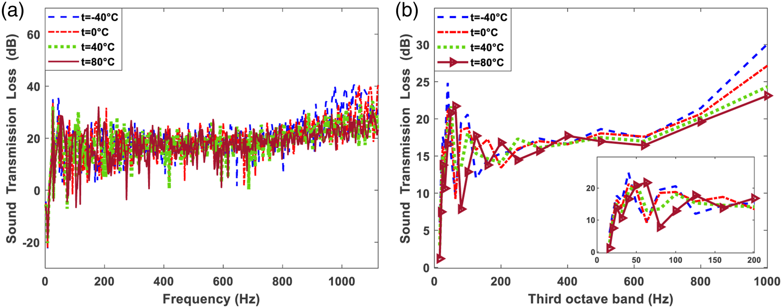

Conclusions

This work has discussed the variability of acoustic characteristic in common frequency region. The sound insulation measurement model is proposed based on the SGM. This model has wide applicability in practical acoustic measurement, and compared with FEM, this method has faster calculation speed and good numerical stability. The vibration velocity of the panel and the sound field inside the suite are also taken into account to explore the acoustic feature and spectrum details of the coupling system. After parametric analysis, the results show that the parameters of the system will all contribute to the discrepancies on the sound transmission characteristic. The main conclusions are summarized as follows:

1. Under four different boundary conditions, the curves with different thickness all show the trend of declining with violent fluctuating and then rising slowly. When the frequency is more than 1000 Hz, the sound insulation performance of the thickest plane is better than the others. The appearance of room modes will weaken the vibration of the structure, resulting in the reduction of radiated sound power and the increase of the STL.

2. The curves of thicker receiving room are more complex, which shows that the mode superposition effect of the components is more obvious. However, the STL of the thicker panel will be significantly reduced when the frequency is over 1800 Hz. This is mainly caused by the modes of the panel. At the modes of the panel, structural resonance will enhance the radiated sound power and reduce the STL. In general, the STL is mainly affected by the parameters of the panel.

3. The change of normal modes caused by high stiffness walls will have a great impact on the sound insulation, and the other curves will keep stable at a certain value after opening shock under weak impedance. When the impedance reaches a value large enough, the acoustic characteristics of the system will not continue to change. At this time, the sound energy density increased significantly, and some sound energy concentration areas will emerge in the room.

4. Sound propagates faster in high-temperature air and its speed is directly proportional to the square root of thermodynamic temperature and the relative humidity almost has no effect on the sound velocity. Besides, by comparing the curves under different temperatures, it is easy to find that the test suite with lower temperature will have better performance of sound insulation when the medium in the acoustic rooms is air.

Footnotes

Declaration of conflicting interests

The author(s) declared no potential conflicts of interest with respect to the research, authorship, and/or publication of this article.

Funding

The author(s) disclosed receipt of the following financial support for the research, authorship, and/or publication of this article: This work is supported by National Natural Science Foundation of China (Grant No. 51805341), Natural Science Foundation of Jiangsu Province (Grant No. BK20180843) and Science and Technology Major Project of Ningbo City (Grant No. 2021Z098).

ORCID iD

Gang Wang

References

Chen

Jin

Liu

. A domain decomposition method for analyzing a coupling between multiple acoustical spaces (L). J Acoust Soc Am 2017; 141: 3018–3021.

Liu

, et al. Acoustic analysis of a rectangular cavity with general impedance boundary conditions. J Acoust Soc Am 2011; 130: 807–817.

Liu

Zhang

Qian

, et al. Influence of stiffeners on plate vibration and radiated noise excited by turbulent boundary layers. Appl Acoust 2014; 80: 28–35.

Federico

Alastair

. Some comments on the numerical analysis of plates and thin-walled structures. Thin-Walled Struct 2008; 46: 975–980.

Wang

Liu

T.S

. The average radiation efficiency of a plate immersed in water with general boundary conditions. Mech Res Commun 2020; 106: 103532.

Wang

Tao

Qiu

, et al. A boundary error sensing arrangement for virtual sound barriers to reduce noise radiation through openings. J Acoust Soc Am 2019; 145: 3695–3702.

Xue

Jin

, et al. Free vibration analysis of porous plates with porosity distributions in the thickness and in-plane directions using isogeometric approach. Int J Mech Sci 2019; 152: 346–362.

Wang

Feng

, et al. A unified approach for predicting the free vibration of an elastically restrained plate with arbitrary holes. Int J Mech Sci 2019; 159: 266–277.

Shi

Jin

, et al. Vibro-acoustic modeling and analysis of a coupled acoustic system comprising a partially opened cavity coupled with a flexible plate. Mech Syst Sig Process 2018; 98: 324–343.

10.

Sadri

Younesian

. Nonlinear free vibration analysis of a plate-cavity system. Thin-Walled Struct 2014; 74: 191–200.

11.

Dai

Xie

Pan

, et al. Strong coupling between magnons confined in a single magnonic cavity. J Appl Phys 2020; 127: 203902.

12.

Chin

. Analytical modelling of structure-borne sound transmission through I-junction using Chebyshev-Ritz method on cascaded rectangular plate-cavity system. Appl Acoust 2019; 143: 171–182.

13.

Wang

Kong

, et al. Acoustic modeling and eigenanalysis of coupled cavities with panels. Mech Syst Sig Process 2022; 165: 108307.

14.

Zhou

Chen

. Sound radiation analysis of functionally graded porous plates with arbitrary boundary conditions and resting on elastic foundation. Int J Struct Stab Dyn 2020; 20: 2050068.

15.

Kong

Wang

, et al. Sound radiation from the plate backed by the rectangular cavity. Int J Mech Sci 2021; 191: 106072.

16.

Guo

. Analysis of sound vibration coupling mechanism of complex plate cavity system. J Appl Mech 2018; 35: 141–146.

17.

Zhang

. A unified approach for predicting sound radiation from baffled rectangular plates with arbitrary boundary conditions. J Sound Vib 2010; 329: 5307–5320.

18.

Chen

Zhang

Ren

, et al. The modeling method of anisotropic U-shaped plate and U-shaped plate-cavity coupled system. Thin-Walled Struct 2021; 172: 108880.

19.

Wang

Zhang

. Analysis of structural acoustic coupling characteristics of closed trapezoidal cavity with elastic plate with different boundary constraints. J Vib Eng 2018; 31: 1021–1030.

20.

Kim

. Solution of coupled acoustic problems: a partially opened enclosure coupled with a membrane and a semi-infinite exterior field. J Sound Vib 2002; 254: 231–244.

21.

Huang

Schröder

. A Bayesian probabilistic approach for damage identification in plate structures using responses at vibration nodes. Mech Syst Sig Process 2021; 146: 106998.

22.

Poblet-Puig

Rodriguez-Ferran

. Modal-based prediction of sound transmission through slits and openings between rooms. J Sound Vib 2013; 332: 1265–1287.

23.

Gagliardini

Roland

Guyader

. The use of a functional basis to calculate acoustic transmission between rooms. J Sound Vib 1991; 145: 457–478.

24.

Dijckmans

Vermeir

. Development of a hybrid wave based-transfer matrix model for sound transmission analysis. J Acoust Soc Am 2020; 133: 2157–2168.

25.

Bravo

Elliott

. Variability of low frequency sound transmission measurements. J Acoust Soc Am 2004; 115: 2986–2997.

26.

Peng

. Sound absorption of a porous material with a perforated facing at high sound pressure levels. J Sound Vib 2018; 425: 01–20.

27.

Xiao

Wen

. Sound transmission loss of metamaterial-based thin plates with multiple subwavelength arrays of attached resonators. J Sound Vib 2012; 331: 5408–5423.

28.

Oudich

Zhou

Assouar

. General analytical approach for sound transmission loss analysis through a thick metamaterial plate. J Appl Phys 2014; 116: 193509.

29.

Deng

Guasch

Maxit

, et al. Transmission loss of plates with multiple embedded acoustic black holes using statistical modal energy distribution analysis. Mech Syst Sig Process 2021; 150: 107262.

30.

Cheng

. Sound radiation and transonic boundaries of a plate with an acoustic black hole. J Acoust Soc Am 2019; 145: 164–172.

31.

Xiang

. Generalization of Sabine’s reverberation theory. J Acoust Soc Am 2020; 148: R5–R6.

32.

ISO 140-3. acoustics, measurement of sound insulation in buildings and of buildings elements. Part 3: laboratory measurements of airborne sound insulation of building elements. 1995.

33.

ISO 140-4: acoustics-measurement of sound insulation in buildings and of building elements-part 4: field measurements of airborne sound insulation between rooms. 1998.

34.

ISO 140-8: acoustics-measurement of sound insulation in buildings and of building elements-part 8: laboratory measurements of the reduction of transmitted impact noise by floor coverings on a heavyweight standard floor. 1997.

35.

Sum

Pan

. Geometrical perturbation of an inclined wall on decay times of acoustic modes in a trapezoidal cavity with an impedance surface. J Acoust Soc Am 2006; 120: 3730–3743.

36.

Ljunggren

. Air-borne sound insulation of single walls at low frequencies: a discussion on the influence of boundary and mounting conditions. Build Acoust 2001; 8: 257–267.

37.

Venkatesham

Tiwari

Munjal

. Analytical prediction of the breakout noise from a rectangular cavity with one compliant wall. J Acoust Soc Am 2008; 124: 2952–2962.

38.

Meissner

. Acoustic energy density distribution and sound intensity vector field inside coupled spaces. J Acoust Soc Am 2012; 132: 228–238.

39.

Azzouz

. Control of sound radiation of an active constrained layer damping plate/cavity system using the structural intensity approach. J Vib Control 2002; 8: 903–918.

40.

. The simplest approach to nonlinear oscillators. Results Phys 2019; 15: 102546.

41.

. Simplified Hamiltonian-based frequency-amplitude formulation for nonlinear vibration system. Facta Univ-Ser Mech 2022; 20: 445–455.

42.

Wang

, et al. A unified procedure for the vibration analysis of elastically restrained Timoshenko beams with variable cross sections. Noise Control Eng J 2020; 68: 38–47.

43.

Beauvais

Pelat

Gautier

, et al. Inverse identification of the acoustic pressure inside a U-shaped pipe line based on acceleration measurements. Mech Syst Sig Process 2021; 160: 107831.

44.

Zhang

Fei

, et al. Modal energy analysis for mechanical systems excited by spatially correlated loads. Mech Syst Sig Process 2018; 111: 362–375.

45.

Huang

Zang

Zhang

, et al. Mode shape transformation for model error localization with modal strain energy. J Sound Vib 2020; 473: 115230.

46.

Fang

Zhang

. An improved hybrid FE-SEA model using modal analysis for the mid-frequency vibro-acoustic problems. Mech Syst Sig Process 2021; 161: 107957.

47.

Kang

Liu

. Comparison of response transmissibility and power spectral density transmissibility on operational modal analysis. Mech Syst Sig Process 2021; 160: 107912.

48.

Mohamed

Wang

. A study of tyre cavity resonance and noise reduction using inner trim. Mech Syst Sig Process 2015; 50–51: 498–509.

49.

Shi

Zuo

Zhong

, et al. Vibration analysis of combined functionally graded cylindrical-conical shells coupled with annular plates in thermal environment. Compos Struct 2022; 294: 115738.

50.

Zhao

Yang

, et al. A new composite plate element for stiffened plate structures via absolute nodal coordinate formulation. Compos Struct 2020; 247: 112431.

51.

Roca

Yago

Cante

, et al. Computational design of locally resonant acoustic metamaterials. Comput Method Appl M 2019; 345: 161–182.

52.

Lee

Kim

. Rigid body modeling issue in acoustical topology optimization. Comput Method Appl M 2009; 198: 1017–1030.

Analytical modeling of the virtual sound insulation measurement suite and research on sound insulation test methods

Abstract

Keywords

Introduction

Theoretical formulations

Acoustic field in the suite

Modeling of the panel

Coupling relationship of the system

Vibration equations of the system

Calculation of the STL

Results and discussions

Model validation

Relationship between impedance and reverberation time T60

Effect of thickness under different boundary conditions

Effect of cavity length under different boundary conditions

Effect of impedance boundary of receiving room

Effect of medium parameters

Conclusions

Footnotes

Declaration of conflicting interests

Funding

ORCID iD

References

Relationship between impedance and reverberation time T₆₀