Galerkin method,ansatz method,and He’s frequency formulation for modeling the forced damped parametric driven pendulum oscillators

Abstract

The forced damped parametric driven pendulum oscillators are analyzed numerically via the Galerkin method (GM) and analytically using both ansatz method (AM) and He’s frequency formulation. One of the most important features of the obtained numerical approximation using GM is that it can recover a large number of different oscillators related to the problem under study. Moreover, the mentioned equation is solved analytically via both AM and He’s frequency formulation. Also, the analytical approximations can recover many different oscillators related to the problem under consideration. Both analytical and numerical approximations are compared with each other and with Runge–Kutta (RK) numerical approximation by estimating both maximum global distance and residual errors. The proposed method can help many authors interested in studying the dynamic problems to explain the mechanics of oscillating to different oscillators in physics, plasma models, engineering, and biological systems.

Introduction

The deep understanding of the mechanism of nonlinear oscillations has an effective role in interpreting the ambiguities of many natural and physical phenomena as well as engineering problems in various fields of science. Accordingly, many researchers have been able to give correct scientific explanations about their scientific experiences based on a deep understanding of the characteristics of these phenomena after the clarity of the ambiguity about the phenomenon under study.^1–5 In the framework of nonlinear dynamics, there is no doubt that the scenario of dynamic mechanism of the pendulum motion is one of the main objects that have deserved more attention in modeling different kind of (non)linear phenomena related to the nonlinear oscillations, chaos, and bifurcations.^6–10 The simple pendulum has been used as a physical model to several solve problems related to many realistic and physical problems, for example, nonlinear plasma oscillations,^11–13 Duffing oscillators,^14–17 Helmholtz oscillations, ¹⁸ the nonlinear equation of wave, ¹⁹ and many other oscillators.^20–25

It is know that the main objective of the numerical approaches is to find some numerical solutions to various realistic physical, engineering, and natural problems, especially when exact solutions are unavailable or extremely difficult to determine. There are many numerical approaches that were used for analyzing the family of the Duffing oscillator and Duffing–Helmholtz oscillator with constant coefficients. It is known that this family is integrable, that is, its exact solution is available in the absence of damping effect. On the other hand, if the damping effect and some others friction forces are taken into account, we get a non–integral differential equation, that is, its exact solution is not available. Therefore, some semi-analytical or/and numerical methods must be used in order to analyze this type of non–integral differential equations to find some approximate analytical and numerical solutions. The parametric driven pendulum equation is one of the non–integral second-order differential equations that govern the motion of a harmonic pendulum under the effect of damping^26,27

$\ddot{\theta }+2\beta \dot{\theta }+\left({\omega }_0^2-Q_0\cos \left(\gamma t\right)\right)\sin \theta =0,$

(1)

where ${\omega }_0=\sqrt{g/l}$ , β = μ/2 ml, and Q₀ = ɛγ²/l. Here, θ denotes the angular displacement, l is the massless pendulum length, m is the mass of the bob suspended in a string, β is the damping coefficient, γ and Q₀ indicate the frequency and excitation amplitude, respectively, and g is the gravity acceleration. The damped parametric driven pendulum is moving harmonically with Q₀ cos (γt) and under the influence of a gravitational restoring force, in addition to the damping force due to air resistance or other damping forces. Equation (1) is derived in details in Ref. ²⁶ and has been analyzed using a midpoint scheme. In addition, the approximate analytical solution to equation (1) in the absence of driven term Q₀ cos (γt) at large angles has been obtained in terms of the Jacobi elliptic functions . ²⁸

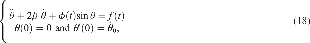
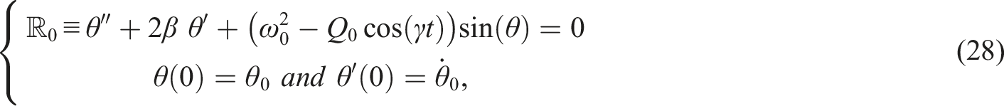
Due to the potential applications of the nonlinear pendulum oscillators, in this work the damped parametric driven pendulum under the influence of a periodic external force in the pivot vertically will be investigated. In this case, the equation of motion becomes

$\ddot{\theta }+2\beta \dot{\theta }+\left({\omega }_0^2-Q_0\cos \left(\gamma t\right)\right)\sin \theta =f\left(t\right).$

(2)

Equation (2) also is not integrable, thus, it will be solved numerically and/or using some ansatz to find some analytical approximations. Using some polynomial approximations to sin θ, we get $\sin \theta \approx \left(\theta -\lambda {\theta }^3\right)$ where λ = 1/6 (for Taylor expansion) or λ = 2/13 (for Chebyshev approximation). Accordingly, equation (2) reduces to the following forced damped Duffing equation with variable coefficients

$\ddot{\theta }+2\beta \dot{\theta }+\left({\omega }_0^2-Q_0\cos \left(\gamma t\right)\right)\left(\theta -\lambda {\theta }^3\right)=f\left(t\right).$

(3)

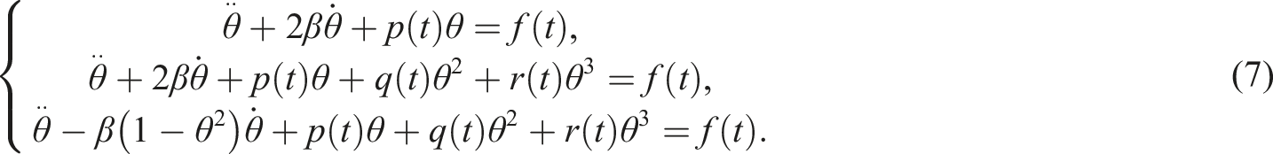
However, in the absence of the driven term Q₀ cos (γt), equation (3) reduces to the forced damped Duffing equation with constant coefficients

$\ddot{\theta }+2\beta \dot{\theta }+{\omega }_0^2\left(\theta -\lambda {\theta }^3\right)=f\left(t\right).$

(4)

In this study, some different analytical and numerical approaches are introduced for analyzing and solving equation (2). In the first, the Galerkin method is employed for analyzing this problem numerically. This method will reduce the second-order differential equation (2) to a system of algebraic nonlinear equations. After that we can solve the obtained system using various method or using MATHEMATICA Package. In the second and third approaches, both ansatz method and He’s frequency formulation are applied for solving this problem analytically. Since this equation is not integrable, so all obtained solutions using both ansatz method and He’s frequency formulation are analytical approximations. Therefore, both maximum global distance and residual errors are estimated for all obtained solutions and compared with RK numerical approximation. The proposed methodology and approximations maybe help many authors for investigating the behavior of realistic pendulum oscillations and many phenomena related to the oscillations such as the motion of atoms and molecules within different materials, oscillations in different plasma systems, etc.

The rest of this work is organized in the following fashion: Galerkin Algorithm for analyzing the equation of motion to the pendulum oscillators is discussed in details in Sec. II. In this section, both unforced and forced damped parametric driven pendulum oscillators are examined. In Sec. (III), the ansatz method is applied for deriving some analytical approximations to the equation of motion. Moreover, In Sec. (IV), He’s frequency formulation is introduced for getting a new formula for the analytical approximation to the equation of motion. In Sec. (V), the obtained approximations for different types of oscillators have been discussed. Also, both maximum global distance error and maximum global residual error have been estimated and discussed for different types of oscillators. Moreover, the impact of physical parameters (coefficients of the physical problem (2)) on the profile of the oscillator have been examined. The obtained results are summarized in Sect. (VI).

Galerkin Algorithm for Analyzing the Damped Pendulum Oscillators

Let us consider a polynomial second-order ode

$\{\begin{array}{c}\ddot{\theta }+2\beta \dot{\theta }+P\left(\theta \right)=0 \\ \theta \left(0\right)=0and\theta \prime \left(0\right)={\dot{\theta }}_0\end{array}$

(5)

where $\theta \equiv \theta \left(t\right)$ and P ≡ P(θ) is a polynomial whose coefficients maybe depend on t, say

$P\left(\theta \right)={\displaystyle \sum _{k=0}^m{a}_k}\left(t\right)x^k.$

(6)

Some particular cases to the i.v.p. (5) could be obtained such as

$\{\begin{array}{c}\stackrel{\mathrm{..}}{\theta }+2\beta \stackrel{.}{\theta }+p\left(t\right)\theta =f\left(t\right),\\ \stackrel{\mathrm{..}}{\theta }+2\beta \stackrel{.}{\theta }+p\left(t\right)\theta +q\left(t\right){\theta }^2+r\left(t\right){\theta }^3=f\left(t\right),\\ \stackrel{\mathrm{..}}{\theta }-\beta (1-{\theta }^2)\stackrel{.}{\theta }+p\left(t\right)\theta +q\left(t\right){\theta }^2+r\left(t\right){\theta }^3=f\left(t\right).\end{array}$

(7)

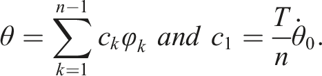
We will use the same idea as for the linear case (7a), that is, we assume an approximate solution to the i.v.p. (5) in the interval 0 ≤ t ≤ T could be defined as

$\theta ={\displaystyle \sum _{k=1}^{n-1}{c}_k}{\phi }_k\left(t\right).$

(8)

where the functions φ _k ≡ φ _k (t) are the so-called linear Galerkin hats, n denotes the number of hat functions and by choosing n ≥ 2 and define the step size h = T/n and let ξ _j = jh = jT/n for j = 0, 1, 2, ⋯n. The hat functions φ _k for 1 ≤ k ≤ n − 1 are defined as follows

${\phi }_k=\{\begin{array}{ll}\frac{t-{\xi }_{k-1}}{h}\hfill & for{\xi }_{k-1}\le t\le {\xi }_k\hfill \\ -\frac{t-{\xi }_{k+1}}{h}\hfill & for{\xi }_k\le t\le {\xi }_{k+1}\hfill \\ 0\hfill & otherwise\hfill \end{array}$

(9)

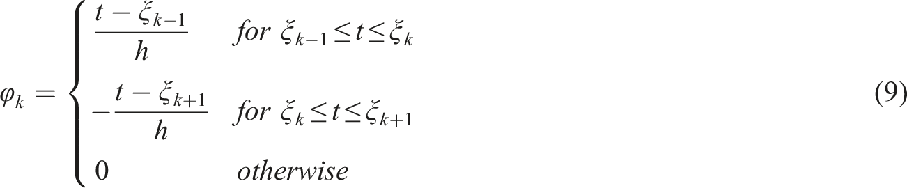
Figure 1 demonstrates the hat functions on the grid ξ ≡ t gives the key for evaluating the weighted residuals. From this figure, we can deduce the values of φ_j−1, φ _j , and φ_j+1 in the intervals $\left[{\xi }_{j-1},{\xi }_j\right]\equiv \left[t_{j-1},t_j\right]$ and $\left[{\xi }_j,{\xi }_{j+1}\right]\equiv \left[t_j,t_{j+1}\right]$ , respectively, as follow

$\begin{array}{cc}{\phi }_{j-1}=-\frac{t}{h}+j+1,& {\phi }_{j-1}^{\prime }=-\frac{1}{h},\\ {\phi }_j=\frac{t}{h}-j,& {\phi }_j^{\prime }=\frac{1}{h},\\ {\phi }_{j+1}=0,& {\phi }_{j+1}^{\prime }=0,\end{array}$

and

$\begin{array}{cc}{\phi }_{j-1}=0,& {\phi }_{j-1}^{\prime }=0,\\ {\phi }_j=-\frac{t}{h}+j+2,& {\phi }_j^{\prime }=-\frac{1}{h},\\ {\phi }_{j+1}=\frac{t}{h}-j-1,& {\phi }_{j+1}^{\prime }=\frac{1}{h},\end{array}$

Figure 1.

Diagram of the hat functions.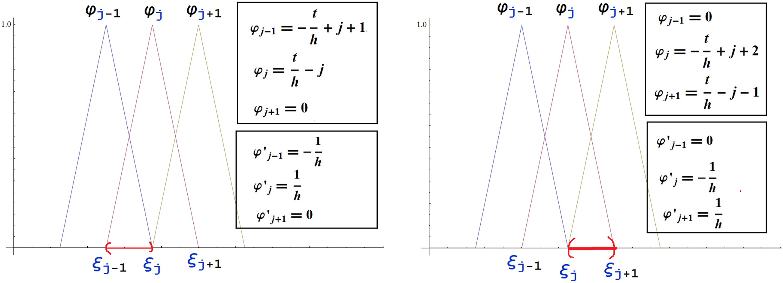

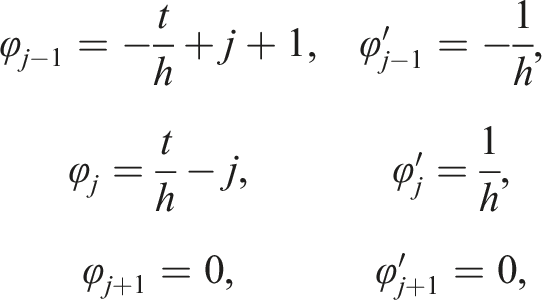
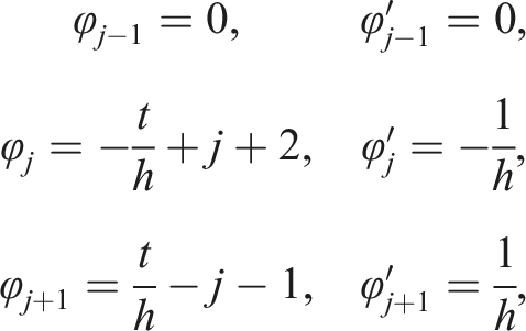
Some properties of the Galerkin hat functions for t ∈ [0, T] could be illustrated as follows

$\begin{array}{cc}{\displaystyle {\int }_0^T{\phi }_j}{\phi }_{k}dt=0,& for \left|j-k\right|\ge 2,\\ {\displaystyle {\int }_0^T{\phi }_j^p}dt=\frac{2T}{\left(p+1\right)n},& for 1\le j\le n-1,\end{array}$

(10)

where p = 1, 2, 3, ⋯.

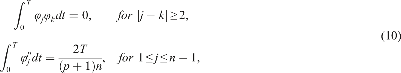
In general, the following integration is obtained

${\displaystyle {\int }_0^T{\phi }_j^r}{\phi }_k^{s}dt=\frac{Tr!s!}{n\left(r+s+1\right)!},$

(11)

for $\left|j-k\right|=1$ and r&s = 0, 1, 2, 3, ⋯.

Moreover, the value of the below integration is derived

${\displaystyle {\int }_0^T{\phi }_j}\left(t\right)x{\left(t\right)}^{N}dt=\frac{T}{\left(k+1\right)\left(k+2\right)n^{N+k+3}}W,$

(12)

where the value of W is given in Appendix (I).

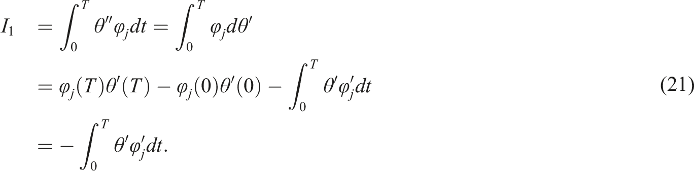
Assuming that a _j (t) ≡ a _j =const, and by using the value of P(x) given in equation (6), we can easily evaluate the following integral

${\displaystyle {\int }_0^{T}P}\left(x\right){\phi }_{j}dt={\displaystyle \sum _{N=0}^m{a}_N}{\displaystyle {\int }_0^T{\phi }_j}x{\left(t\right)}^{N}dt,$

(13)

for any j.

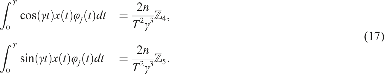
Some others useful formulas that can be used for analyzing the different equations of motion for various pendulum oscillators via Galerkin method are introduced

${\displaystyle {\int }_0^T{t}^r}\theta \left(t\right){\phi }_j\left(t\right)dt=\frac{n^{-r-1}{T}^{r+1}}{{\displaystyle \prod }_{i=1}^3\left(r+i\right)}{\mathbb{Z}}_1,$

(14)

${\displaystyle {\int }_0^T{t}^r}{\theta }^2\left(t\right){\phi }_j\left(t\right)dt=\frac{n^{-r-1}{T}^{r+1}}{{\displaystyle \prod }_{i=1}^4\left(r+i\right)}{\mathbb{Z}}_2,$

(15)

${\displaystyle {\int }_0^T{t}^r}{\theta }^3\left(t\right){\phi }_j\left(t\right)dt=\frac{n^{-r-1}{T}^{r+1}}{{\displaystyle \prod }_{i=1}^5\left(r+i\right)}{\mathbb{Z}}_3,$

(16)

where the functions ${\mathbb{Z}}_1-{\mathbb{Z}}_5$ are given in Appendix (II).

The formulas (14)-(16) are used for evaluating the weighted residuals in the case when the coefficients a _k (t) in (6) are polynomials in t. For example, the variable-coefficients forced damped Helmholtz–Duffing oscillator: $\ddot{\theta }+2\beta \dot{\theta }+\left(2t^3-1\right)\theta +5t{\theta }^2+r\left(t\right){\theta }^3=f\left(t\right)$ .

Moreover, some relations related to the Galerkin hats and trigonometric functions are defined as

$\begin{array}{ll}{\displaystyle {\int }_0^T\cos }\left(\gamma t\right)x\left(t\right){\phi }_j\left(t\right)dt\hfill & =\frac{2n}{T^2{\gamma }^3}{\mathbb{Z}}_4,\hfill \\ {\displaystyle {\int }_0^T\sin }\left(\gamma t\right)x\left(t\right){\phi }_j\left(t\right)dt\hfill & =\frac{2n}{T^2{\gamma }^3}{\mathbb{Z}}_5.\hfill \end{array}$

(17)

For example, the forced damped Mathieu–Duffing oscillator: $\ddot{\theta }+2\beta \dot{\theta }+\left(a+b\cos \left(\gamma t\right)\right)\theta +\beta {\theta }^3=f\left(t\right)$ may be solved using he relation (17) may be solved using (17).

Galerkin method for anatomy the forced damped pendulum oscillators

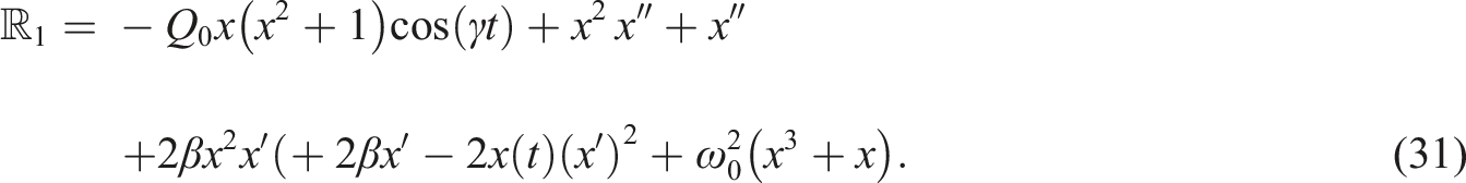
Now, let us apply the Galerkin method for analyzing the forced damped parametric driven pendulum i.v.p.

$\{\begin{array}{c}\ddot{\theta }+2\beta \dot{\theta }+\varphi \left(t\right)\sin \theta =f\left(t\right)\\ \theta \left(0\right)=0\text{ and }\theta \prime \left(0\right)={\dot{\theta }}_0,\end{array}$

(18)

where $\theta \equiv \theta \left(t\right)$ and f(t) = F cos (Ωt).

Assuming that there exists some T > 0 which satisfies θ(0) = θ(T) = 0. Now, we try to find an approximate solution to the i.v.p. (18) in the ansatz form

$\theta ={\displaystyle \sum _{k=1}^{n-1}{c}_k}{\phi }_{k}and{c}_1=\frac{T}{n}{\dot{\theta }}_0.$

Let us define the residual $ℝ\left(t\right)$ as

$ℝ\left(t\right)\equiv \theta ″+2\beta \theta \prime +\varphi \left(t\right)\sin \theta -f\left(t\right)=0.$

(19)

Multiplying both sides of equation (19) by φ _j , and integrating the obtained equation on the interval $\left[0,T\right]$ , we get

${\displaystyle {\int }_0^Tℝ}\left(t\right){\phi }_{j}dt=I_1+2\beta I_2+I_3-I_4=0$

(20)

where

$\begin{array}{cc}{I}_1={\displaystyle {\int }_0^T\theta ″}{\phi }_{j}dt,& I_2={\displaystyle {\int }_0^T\theta \prime }{\phi }_{j}dt,\\ I_3={\displaystyle {\int }_0^T\varphi }\left(t\right)\sin \theta {\phi }_{j}dt,& I_4={\displaystyle {\int }_0^{T}f}\left(t\right){\phi }_{j}dt.\end{array}$

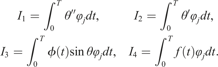
Now we can integrate equation (20) term by term according to the Galerkin method and depending on the above mentioned relations

$\begin{array}{ll}{I}_1\hfill & ={\displaystyle {\int }_0^T\theta ″}{\phi }_{j}dt={\displaystyle {\int }_0^T{\phi }_j}d\theta \prime \hfill \\ \hfill & ={\phi }_j\left(T\right)\theta \prime \left(T\right)-{\phi }_j\left(0\right)\theta \prime \left(0\right)-{\displaystyle {\int }_0^T\theta \prime }{\phi }_j^{\prime }dt\hfill \\ \hfill & =-{\displaystyle {\int }_0^T\theta \prime }{\phi }_j^{\prime }dt.\hfill \end{array}$

(21)

Using the value of θ given in equation (8), and taking the value of the relation φ _r φ _s = 0 for $\left|r-s\right|\ge 2$ into account, we obtain

$\theta \prime {\phi }_j^{\prime }={\displaystyle \sum _{k=1}^{n-1}{c}_k}{\phi }_k^{\prime }{\phi }_j^{\prime }=c_{j-1}{\phi }_{j-1}^{\prime }{\phi }_j^{\prime }+c_j{\phi }_j^{\prime }{\phi }_j^{\prime }+c_{j+1}{\phi }_{j+1}^{\prime }{\phi }_j^{\prime }.$

(22)

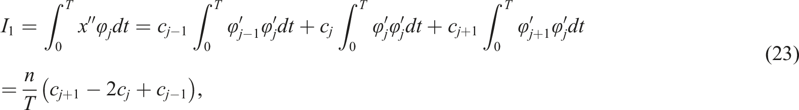
Inserting equation (22) into equation (21) give us

$\begin{array}{l}{I}_1={\displaystyle {\int }_0^{T}x″}{\phi }_{j}dt=c_{j-1}{\displaystyle {\int }_0^T{\phi }_{j-1}^{\prime }}{\phi }_j^{\prime }dt+c_j{\displaystyle {\int }_0^T{\phi }_j^{\prime }}{\phi }_j^{\prime }dt+c_{j+1}{\displaystyle {\int }_0^T{\phi }_{j+1}^{\prime }}{\phi }_j^{\prime }dt\\ =\frac{n}{T}\left(c_{j+1}-2c_j+c_{j-1}\right),\end{array}$

(23)

for 1 ≤ j ≤ n − 1. Note that formula (23) remains valid for j = 1 and j = n − 1.

Following the same procedure as above, the value of the integral I₂ can be easily obtained

$I_2={\displaystyle {\int }_0^T\theta \prime }{\phi }_{j}dt=c_{j+1}-c_{j-1,}$

(24)

for 1 ≤ j ≤ n − 1.

The integral value of I₄ can be evaluated as follows

$I_4={\displaystyle {\int }_0^{T}f}\left(t\right){\phi }_{j}dt=F{\displaystyle {\int }_0^T\cos }\left(\mathrm{\Omega }t\right){\phi }_{j}dt=I_{4a}+I_{4b}+I_{4c},$

where

$\begin{array}{ll}{I}_{4a}\hfill & =\frac{4nF}{T{\mathrm{\Omega }}^2}{\hspace{0.17em}\sin }^2\left(\frac{\mathrm{\Omega }}{2n}T\right)\cos \left(\frac{\mathrm{\Omega }}{n}T\right),forj=1\hfill \\ I_{4b}\hfill & =-\frac{2nF}{T{\mathrm{\Omega }}^2}\left[\cos \left(\frac{\mathrm{\Omega }}{n}T\right)-1\right]\cos \left(\frac{\mathrm{\Omega }}{n}jT\right),for1<j<n-1\hfill \\ I_{4c}\hfill & =-\frac{nF}{T{\mathrm{\Omega }}^2}\left[\cos \left(\frac{\left(n-2\right)\mathrm{\Omega }}{n}T\right)-2\cos \left(\frac{\left(n-1\right)\mathrm{\Omega }}{n}T\right)+\cos \left(\mathrm{\Omega }T\right)\right],forj=n-1\hfill \end{array}$

(25)

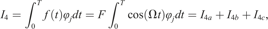
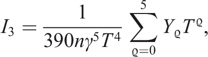
Our next aim is to evaluate the integral value of I₃

$\begin{array}{l}{I}_3={\displaystyle {\int }_0^T\varphi \left(t\right)}\sin \left(\theta {\phi }_j\right)dt=\left({\displaystyle {\int }_{{\xi }_{j-1}}^{{\xi }_j}}+{\displaystyle {\int }_j^{j+1}}\right)\varphi \left(t\right)\sin \left(\theta {\phi }_j\right)dt\\ \approx {\displaystyle {\int }_{{\xi }_{j-1}}^{{\xi }_j}\varphi \left(t\right)}\left(\theta -\frac{2}{13}\hspace{0.17em}{\theta }^3\right){\phi }_{j}dt+{\displaystyle {\int }_{{\xi }_j}^{{\xi }_{j+1}}\varphi \left(t\right)}\left(\theta -\frac{2}{13}\hspace{0.17em}{\theta }^3\right){\phi }_{j}dt,\\ \theta \left(t\right)=c_{j-1}{\phi }_{j-1}{\phi }_j+c_j{\phi }_j^2+c_{j+1}{\phi }_{j+1}{\phi }_j.\end{array}$

(26)

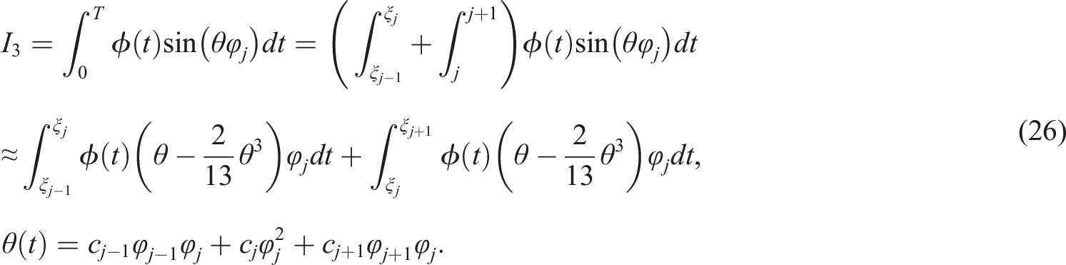
Using the above relations and after some tedious but straightforward calculations, we obtain

$I_3=\frac{1}{390n{\gamma }^5{T}^4}{\displaystyle \sum _{\mathrm{\varrho }=0}^5{Y}_{\mathrm{\varrho }}}{T}^{\mathrm{\varrho }},$

where Y _ϱ is given in Appendix (III).

Finally, the system of nonlinear transcendental equations to be solved is

$\frac{1}{nT}\left(c_{j-1}-2c_j+c_{j+1}\right)+2\beta \left(c_{j+1}-c_{j-1}\right)+I_3-I_4=0,$

(27)

where i = 2, 3, …, n − 1, c₀ = c _n = 0, and $c_1=T{\dot{\theta }}_0/n$ .

We will have $\left(n-1\right)$ unknowns constants that need to be determined, namely, c₂, c₃, ⋯ , c_n−1, and T. The initial guess value of T is some positive number and the initial guess values of each c _j may be chosen randomly on the interval [ − 1, 1]. And by solving the obtained system of the nonlinear transcendental equations, we get some zero of the solution, that is, the value of T for which the graph of the solution crosses the t-axis. Anyway, the GM may give us one or more zeros of the solution.

Analytical Approaches

Here, both Ansatz method (AM) and He’s frequency formulation can be applied for deriving some analytical approximations to the nonlinear pendulum equation of motion.

First approach: Ansatz Method

To find an analytical approximation to the i.v.p. (18), the proposed method (ansatz method (AM)) is summarized in the following steps

Step (1) First let F = 0, then the i.v.p. (18) reduces to the following i.v.p.

$\{\begin{array}{c}{ℝ}_0\equiv \theta ″+2\beta \theta \prime +\left({\omega }_0^2-Q_0\cos \left(\gamma t\right)\right)\sin \left(\theta \right)=0\\ \theta \left(0\right)={\theta }_{0}and\theta \prime \left(0\right)={\dot{\theta }}_0,\end{array}$

(28)

• Step (2) Assuming that the solution of the i.v.p. (28) is given by the ansatz

$\theta =2{\tan }^{-1}\left(x\right),$

(29)

where x ≡ x(t).

• Step (3) Inserting the ansatz (29) in equation (28), we have

${ℝ}_0=\frac{2}{{\left(x{\left(t\right)}^2+1\right)}^2}\left({ℝ}_1\right),$

(30)

with

$\begin{array}{l}{ℝ}_1=-Q_{0}x\left(x^2+1\right)\cos \left(\gamma t\right)+x^{2}x″+x″\\ +2\beta x^{2}x\prime (+2\beta x\prime -2x\left(t\right){\left(x^{\prime }\right)}^2+{\omega }_0^2\left(x^3+x\right).\end{array}$

(31)

• Step (4) Assuming the solution of ${ℝ}_1=0$ , is given by

$x\left(t\right)=c_0\exp \left(-\beta t\right)\cos \left(f+c_1\right).$

(32)

where c₀ and c₁ are two undetermined constant and f ≡ f(t) is a time function.

• Step (5) Inserting ansatz (32) into equation (31), we get

${ℝ}_1={ℝ}_2\cos \left(f+c_1\right)+h.o.t.$

(33)

with

${ℝ}_2=\begin{array}{c}-\frac{1}{4}\hspace{0.17em}{c}_0\hspace{0.17em}{e}^{-3\beta t}\left(5c_0^2+4e^{2\beta t}\right){\left(f^{\prime }\right)}^2-\frac{1}{4}\hspace{0.17em}{c}_0\hspace{0.17em}{Q}_0{e}^{-3\beta t}\left(3c_0^2+4e^{2\beta t}\right)\cos \left(\gamma t\right)\\ -\frac{1}{4}\hspace{0.17em}{c}_0\hspace{0.17em}{\beta }^2{e}^{-3\beta t}\left(9c_0^2+4e^{2\beta t}\right)+\frac{1}{4}\hspace{0.17em}{c}_0\hspace{0.17em}{\omega }_0^2{e}^{-3\beta t}\left(3c_0^2+4e^{2\beta t}\right),\end{array}$

(34)

where h.o.t. indicates the higher-order terms.

• Step (6) For ${ℝ}_2=0$ , we get an ode in f^′ which leads to

$f\left(t\right)={\displaystyle {\int }_0^t\sqrt{\frac{4\left({\omega }_0^2-{\beta }^2-Q_0\cos \left(\gamma \tau \right)\right)e^{2\beta \tau }+3c_0^2\left(3{\beta }^2-{\omega }_0^2+Q_0\cos \left(\gamma \tau \right)\right)}{5c_0^2+4e^{2\beta \tau }}}}d\tau ,$

(35)

where constants c₀ and c₁ can be determined from the ICs θ(0) = θ₀ and $\theta \prime \left(0\right)={\dot{\theta }}_0$ .

• Step (7) Now, let us retune to the i.v.p. (18) and suppose that its analytical approximation is given by

$\theta \left(t\right)=2{\tan }^{-1}\left(c_0\exp \left(-\beta t\right)\cos \left(f+c_1\right)\right)+\frac{F_0\cos \left(\mathrm{\Omega }t\right)}{{\omega }_0^2-Q_0-{\mathrm{\Omega }}^2},$

(36)

• Step (8) The integration of equation (35) may be approximated as follows

$\begin{array}{ll}f\left(t\right)\hfill & ={\displaystyle {\int }_0^t\sqrt{\frac{4\left({\omega }_0^2-{\beta }^2-Q_0\cos \left(\gamma \tau \right)\right)e^{2\beta \tau }+3c_0^2\left(3{\beta }^2-{\omega }_0^2+Q_0\cos \left(\gamma \tau \right)\right)}{5c_0^2+4e^{2\beta \tau }}}}d\tau \hfill \\ \hfill & \approx {\displaystyle {\int }_0^t\sqrt{\frac{4w_0{e}^{2\beta \tau }+3c_0^2\left(3{\beta }^2-{\omega }_0^2+Q_0\mu \right)}{5c_0^2+4e^{2\beta \tau }}}}d\tau \hfill \\ \hfill & =\frac{\sqrt{w_0}}{\beta }\left[\begin{array}{c}{\tanh }^{-1}\left(W_1\left(t\right)\right)-{\tanh }^{-1}\left(W_1\left(0\right)\right)\\ +\sqrt{P+1}\left({\tanh }^{-1}\left(\frac{W_1\left(0\right)}{\sqrt{P+1}}\right)-{\tanh }^{-1}\left(\frac{W_1\left(t\right)}{\sqrt{P+1}}\right)\right)\end{array}\right],\hfill \end{array}$

(37)

with

$\begin{array}{l}{w}_0={\omega }_0^2-{\beta }^2-\mu Q_0,\hfill \\ W_1\left(t\right)=\sqrt{\frac{P}{Q{e}^{2\beta t}+1}+1,}\hfill \\ \mu =\frac{1}{T}{\displaystyle {\int }_0^T\cos }\left(\gamma t\right)dt=\frac{\sin \left(T\gamma \right)}{T\gamma },\hfill \\ P=\frac{6{\beta }^2}{5w_0}-\frac{8}{5}, Q=\frac{4}{5c_0^2}.\hfill \end{array}$

(38)

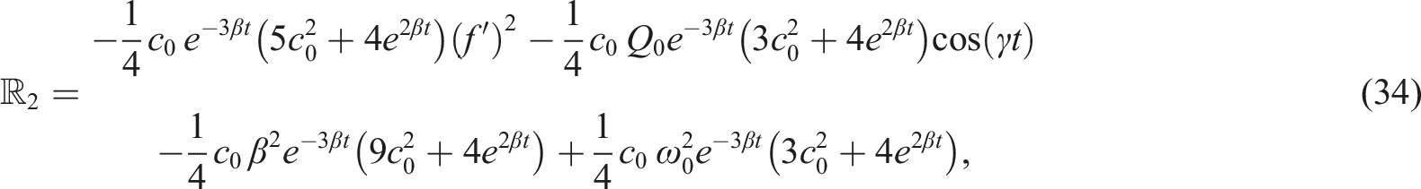
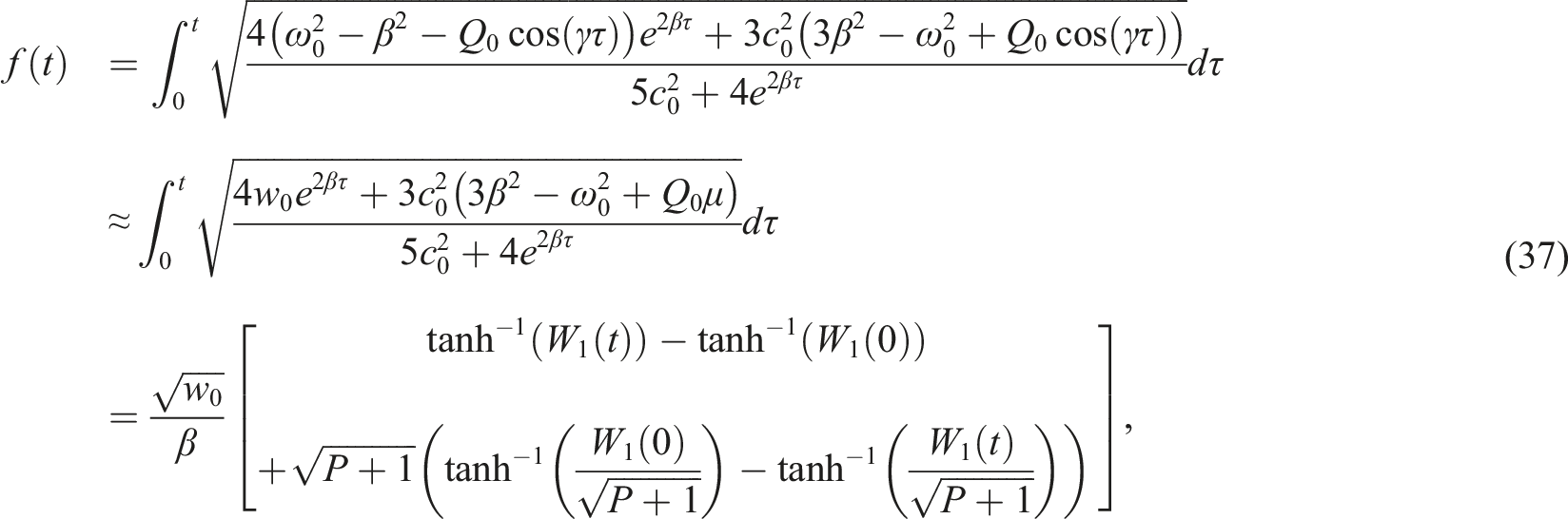
The constants c₀ and c₁ are found from the ICs θ(0) = θ₀ and $\theta \prime \left(0\right)={\dot{\theta }}_0$ .

Second approach: He’s frequency formulation

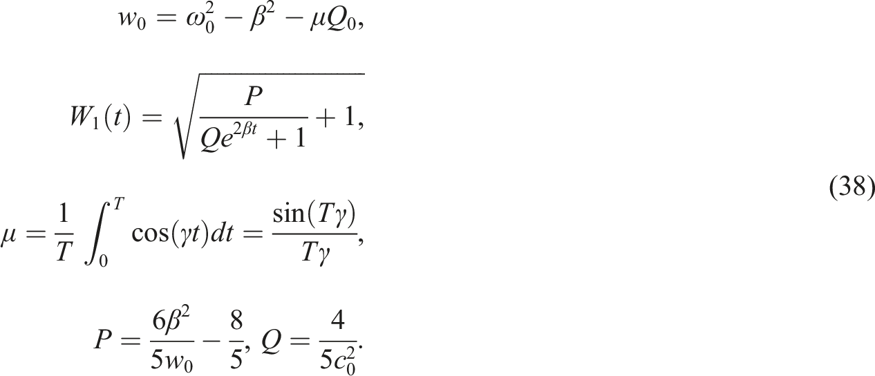
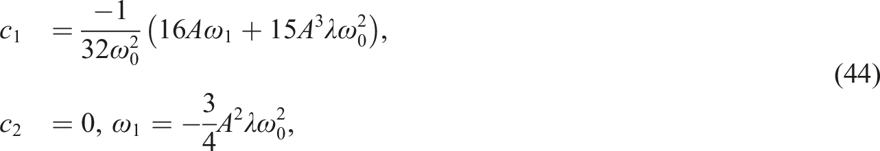
This was devoted for analyzing many problems related to the different pendulum oscillators .^29–33 The algorithm of this approach can be summarized in the following brief steps based on the published papers about this method

Step (1) Let us define the following residual function

$R\left(t\right)=\theta ″+2\beta \theta \prime +\left({\omega }_0^2-Q_0\cos \left(\gamma t\right)\right)\sin \theta -F\cos \left(\mathrm{\Omega }t\right).$

(39)

• Step (2) Using Taylor expansion or Chebyshev approximation for $\sin \theta \approx \left(\theta -\lambda {\theta }^3\right)$ , then we have

$R\left(t\right)\approx \theta ″+2\beta \theta \prime +\left({\omega }_0^2-Q_0\cos \left(\gamma t\right)\right)\left(\theta -\lambda {\theta }^3\right)-F\cos \left(\mathrm{\Omega }t\right),$

(40)

• where λ = 1/6 (for Taylor expansion) or λ = 2/13 (for Chebyshev approximation).

• Step (3) For β = 0 and F₀ = 0, the following homotopy is introduced

$H_p=\theta ″+{\omega }_0^2\theta +p\left[-\lambda {\theta }^3\left({\omega }_0^2-Q_0\cos \left(\gamma t\right)\right)-Q_0\theta \cos \left(\gamma t\right)\right].$

(41)

Assuming the solution is defined by the following ansatz

$\theta =A\cos \left(\tau \right)+pu\left(\tau \right),$

(42)

where $\tau =\sqrt{{\omega }_0^2+p{\omega }_1}t$ and ω₁ will be determined later and for simplicity we can use $u\equiv u\left(\tau \right)$ .

• Step (4) Inserting solution (42) into H _p = 0 (given in equation (41)) and after tedious calculations and in order to avoid secularity, then we obtain the following ode in u for p = 1,

$\begin{array}{l}{\omega }_0^2\left(u″+u-A^3\lambda {\cos }^3\left(\tau \right)\right)+A\cos \left(\tau \right)\left(-{\omega }_1-Q_0\cos \left(\frac{\gamma \tau }{{\omega }_0}\right)+A^2{Q}_0\lambda {\cos }^2\left(\tau \right)\cos \left(\frac{\gamma \tau }{{\omega }_0}\right)\right)=0.\end{array}$

(43)

• Step (5) Integrating equation (43) twice over τ, we obtain a huge value for u with two constants $\left(c_1,c_2\right)$ . To get the values of the integration constants and the value of ω₁, we equate the coefficients of cos(τ) and sin(τ) to zero which lead to

$\begin{array}{ll}{c}_1\hfill & =\frac{-1}{32{\omega }_0^2}\left(16A{\omega }_1+15A^3\lambda {\omega }_0^2\right),\hfill \\ c_2\hfill & =0,{\omega }_1=-\frac{3}{4}{A}^2\lambda {\omega }_0^2,\hfill \end{array}$

(44)

• Step (6) Then the value of u is obtained as

$\begin{array}{ll}u\hfill & =-\frac{1}{32}{A}^3\lambda \cos \left(3\tau \right)+\frac{A{Q}_0}{2\left(-20{\gamma }^3{\omega }_0^2+{\gamma }^5+64\gamma {\omega }_0^4\right)}\times \hfill \\ \hfill & \left[\begin{array}{c}{\gamma }^3\cos \left(\tau \right)\left(A^2\lambda \cos \left(2\tau \right)+A^2\lambda -2\right)\cos \left(\frac{\gamma \tau }{{\omega }_0}\right)\\ +2{\omega }_0\left(\begin{array}{c}\sin \left(\tau \right)\sin \left(\frac{\gamma \tau }{{\omega }_0}\right)\left({\gamma }^2\left(3A^2\lambda \cos \left(2\tau \right)+3A^2\lambda -2\right)+8{\omega }_0^2\left(4-3A^2\lambda \right)\right)\\ +2\gamma {\omega }_0\cos \left(\tau \right)\left(2A^2\lambda \cos \left(2\tau \right)-7A^2\lambda +8\right)\cos \left(\frac{\gamma \tau }{{\omega }_0}\right)\end{array}\right)\end{array}\right].\hfill \end{array}$

(45)

• Step (7) He’s frequency–amplitude formulation reads

${\omega }^2={\omega }_0^2+{\omega }_1={\omega }_0^2\left(1-\frac{3}{4}\lambda A^2\right).$

(46)

• Step (8) In order to get the solution to the damped oscillator, we replace A by A exp (−βt) and then we get the following generalized frequency–amplitude formulation

${\omega }^2=w\prime {\left(t\right)}^2={\omega }_0^2\left(1-\frac{3}{4}\lambda A^2\exp \left(-2\beta \tau \right)\right).$

(47)

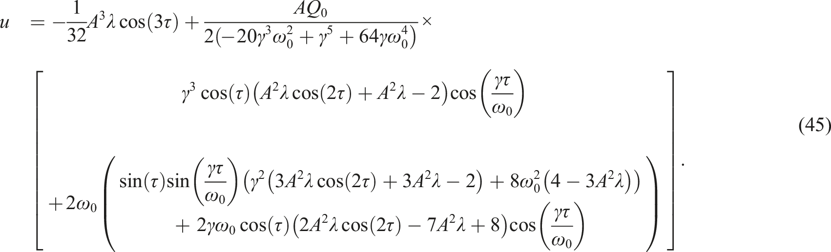
Finally, the solution to the unforced damped oscillator reads

$\theta \left(t\right)=A\exp \left(-\beta t\right)\cos (w\left(t\right))+u(w\left(t\right)),$

(48)

with

$w\left(t\right)=B+{\omega }_0{\displaystyle {\int }_0^t\sqrt{1-\frac{3}{4}\lambda A^2\exp \left(-2\beta \tau \right)}}d\tau ,$

(49)

and in the expression (45), the constant A is replaced by A exp (−βt). The values of the constants A and B are obtained from the ICs.

• Step (9) For the forced damped case $\left(\beta \ne 0\hspace{0.17em}\hspace{0.17em}\&\hspace{0.17em}\hspace{0.17em}F\ne 0\right)$ , the solution of the i.v.p. (18) is defined as

$\theta \left(t\right)=\phi \left(t\right)+c\cos \left(\mathrm{\Omega }t\right),$

(50)

where $\phi \left(t\right)$ represents the solution of unforced damped case, that is, $\phi \equiv \phi \left(t\right)=\theta \left(t\right)=A\exp \left(-\beta t\right)\cos \left(w\left(t\right)\right)+u\left(w\left(t\right)\right)$ given in equation (48) and the coefficient c will be determined later.

• Step (10) By inserting solution (50) into equation (39), taking the following value of φ into consideration

$\phi ″=-2\beta \phi \prime -\left({\omega }_0^2-Q_0\cos \left(\gamma t\right)\right)\left(\phi -\lambda {\phi }^3\right),$

we get

$\begin{array}{l}\left(-\frac{3}{4}\hspace{0.17em}{c}^3\lambda {\omega }_0^2-3c\lambda {\omega }_0^2\phi {\left(t\right)}^2+c{\omega }_0^2-c{\mathrm{\Omega }}^2-F\right)\cos \left(t\mathrm{\Omega }\right)\\ +\left(\frac{3}{8}\hspace{0.17em}{c}^3\lambda +\frac{3}{2}c\lambda \phi {\left(t\right)}^2-\frac{c}{2}\right)Q_0\cos \left(\gamma t-t\mathrm{\Omega }\right)\\ +\left(\frac{3}{8}\hspace{0.17em}{c}^3\lambda +\frac{3}{2}c\lambda \phi {\left(t\right)}^2-\frac{c}{2}\right)Q_0\cos \left(\gamma t+t\mathrm{\Omega }\right)\\ +\frac{3}{4}\hspace{0.17em}{c}^2\lambda Q_0\phi \left(t\right)\cos \left(\gamma t-2t\mathrm{\Omega }\right)+\frac{3}{4}\hspace{0.17em}{c}^2\lambda Q_0\phi \left(t\right)\cos \left(\gamma t+2t\mathrm{\Omega }\right)\\ +\frac{3}{2}\hspace{0.17em}{c}^2\lambda Q_0\phi \left(t\right)\cos \left(\gamma t\right)+\frac{1}{8}\hspace{0.17em}{c}^3\lambda Q_0\cos \left(\gamma t-3t\mathrm{\Omega }\right)\\ +\frac{1}{8}\hspace{0.17em}{c}^3\lambda Q_0\cos \left(\gamma t+3t\mathrm{\Omega }\right)-\frac{3}{2}\hspace{0.17em}{c}^2\lambda {\omega }_0^2\phi \left(t\right)\cos \left(2t\mathrm{\Omega }\right)\\ -\frac{3}{2}\hspace{0.17em}{c}^2\lambda {\omega }_0^2\phi \left(t\right)-\frac{1}{4}\hspace{0.17em}{c}^3\lambda {\omega }_0^2\cos \left(3t\mathrm{\Omega }\right)+2\beta c\lambda t^3{\mathrm{\Omega }}^4-2\beta ct{\mathrm{\Omega }}^2=0.\end{array}$

(51)

• Step (11) From the coefficient of cos (tΩ) in expression (51) and for φ(0) = 0, we have

$-\frac{3}{4}\hspace{0.17em}{c}^3\lambda {\omega }_0^2+c{\omega }_0^2-c{\mathrm{\Omega }}^2-F=0.$

(52)

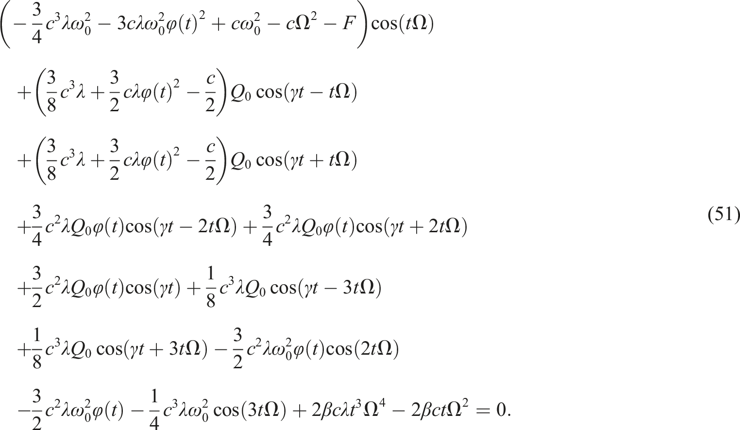
By solving equation (52) using the following mathematica commands

$Solve\left[PadeApproximant\left[-\frac{3}{4}\hspace{0.17em}{c}^3\lambda {\omega }_0^2+c{\omega }_0^2-c{\mathrm{\Omega }}^2-F,\left\{c,0,\left\{1,n\right\}\right\}\right]==0,c\right]$

the value of c can be obtained for different values to n = 1, 2, 3, ⋯.

RESULTS AND DISCUSSION

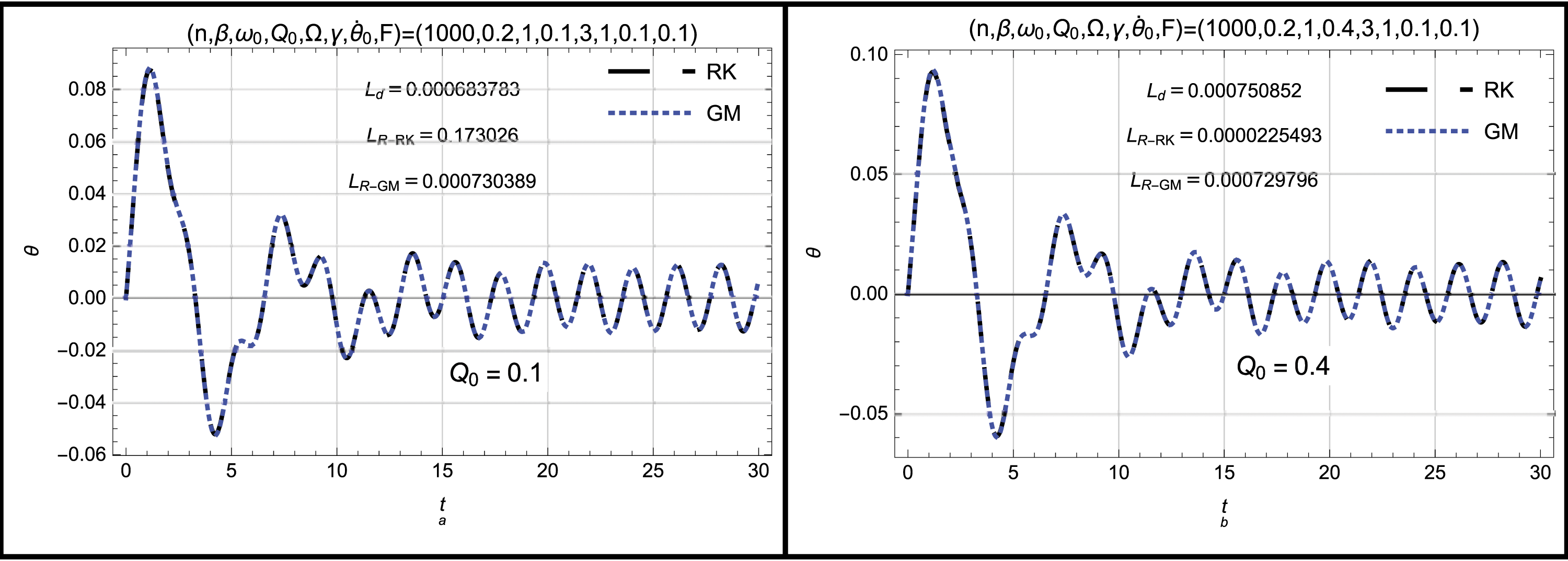
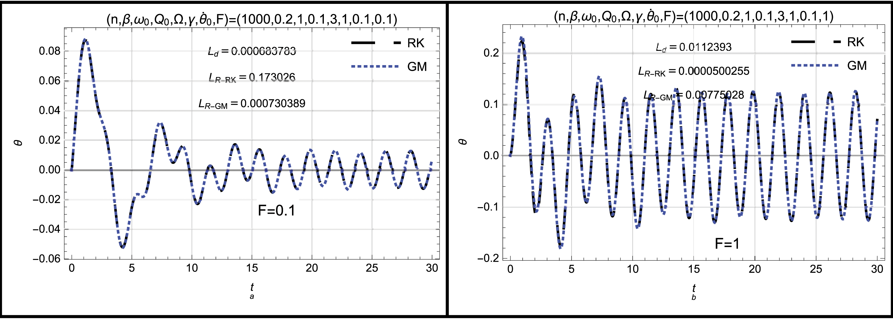
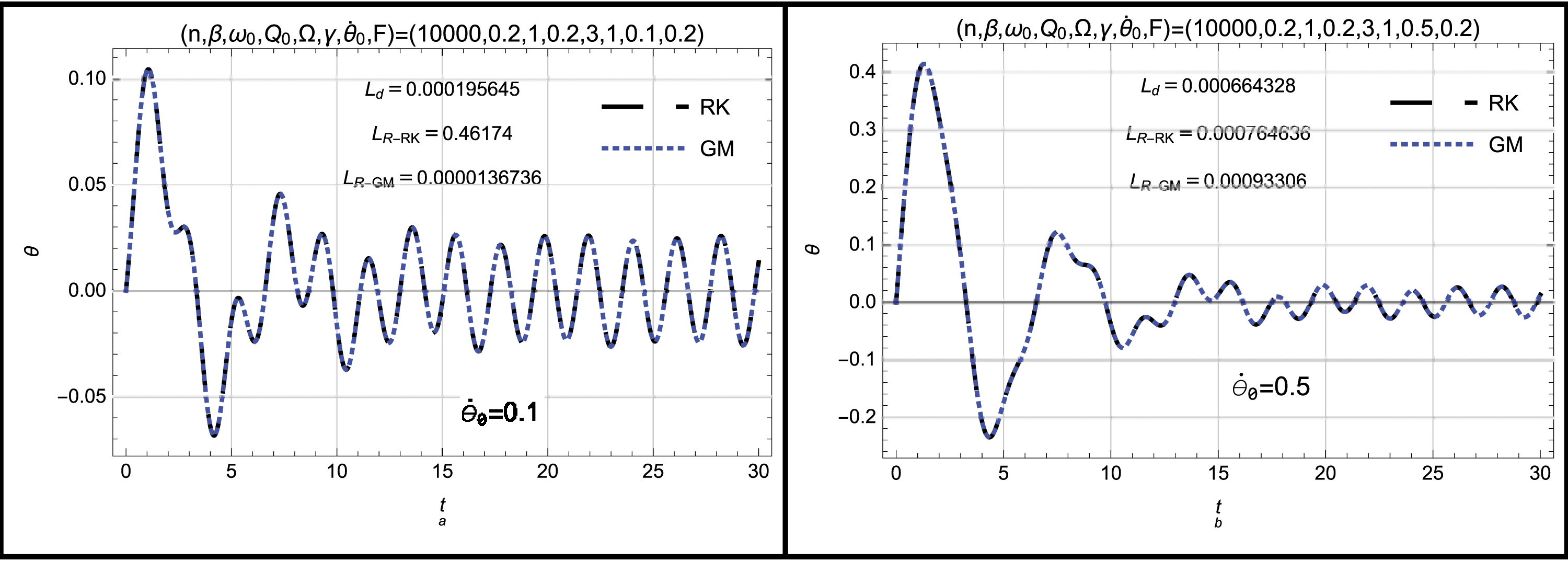
For numerical results, we can discuss different cases for the nonlinear pendulum oscillators depending on the initial conditions $\left({\theta }_0,{\dot{\theta }}_0\right)=\left(\mathrm{0,0.1}\right)$ and the different values of the physical parameters $\left(\beta ,{\omega }_0,Q_0,\gamma ,\mathrm{\Omega },{\dot{\theta }}_0,F\right)$ at fixed $\left({\omega }_0,\gamma ,\mathrm{\Omega }\right)=\left(\mathrm{1,1,2}\right)$ using both Galerkin and RK numerical approximations as follow

• In the first case, the variable-coefficients forced damped Duffing oscillator for $\left(\beta ,F,Q_0\right)=\left(0.1,0.1,0.1\right)$ is investigated as shown in Figure 2(a) using the

• In the absence of forced term (F = 0), the variable-coefficients unforced damped Duffing oscillator is presented as illustrated in Figure 2(b) for $\left(\beta ,F,Q_0\right)=\left(0.1,\mathrm{0,0.1}\right)$ .

• Also, the variable-coefficients forced undamped Duffing oscillator in the absence damping term (β = 0) is discussed for $\left(\beta ,F,Q_0\right)=\left(\mathrm{0,0.1},0.1\right)$ as demonstrated in Figure 2(c).

• Moreover, the forced damped parametric pendulum oscillator/or the constant-coefficients forced damped Duffing oscillator in the absence of the excitation amplitude (Q₀ = 0) is discussed for $\left(\beta ,F,Q_0\right)=\left(0.1,0.1,0\right)$ as demonstrated in Figure 2(d).

Figure 2.

The numerical approximations to the i.v.p. (18) using both GM and RK numerical method for different values of $\left(\beta ,Q_0\text{, }F\right)$ are plotted in $\left(\theta ,t\right)-$ plane.

In all cases, we make a comparison between the Galerkin approximations and the RK numerical solutions graphically as shown in Figure 2. Also, both maximum global distance error according to the following formula

$L_d=\underset{0\le t\le T}{\max }\left|\text{RK}-{\theta }_{\text{M}}\right|,$

and the following maximum global residual error

$\begin{array}{l}{L}_{R|RK}=\underset{0\le t\le T}{\max }\left|ℝ{\left(t\right)}_{RK}\right|,\hspace{1em}{L}_{R|GM}=\underset{0\le t\le T}{\max }\left|ℝ{\left(t\right)}_M\right|,\hfill \end{array}$

are estimated for both Galerkin and RK numerical approximations in the whole time domain 0 ≤ t ≤ 30 as elucidated in Table 1. It is noticed from the results given in Table 1 that the GM sometimes gives results with accuracy better than the RK numerical solution.

Table 1.

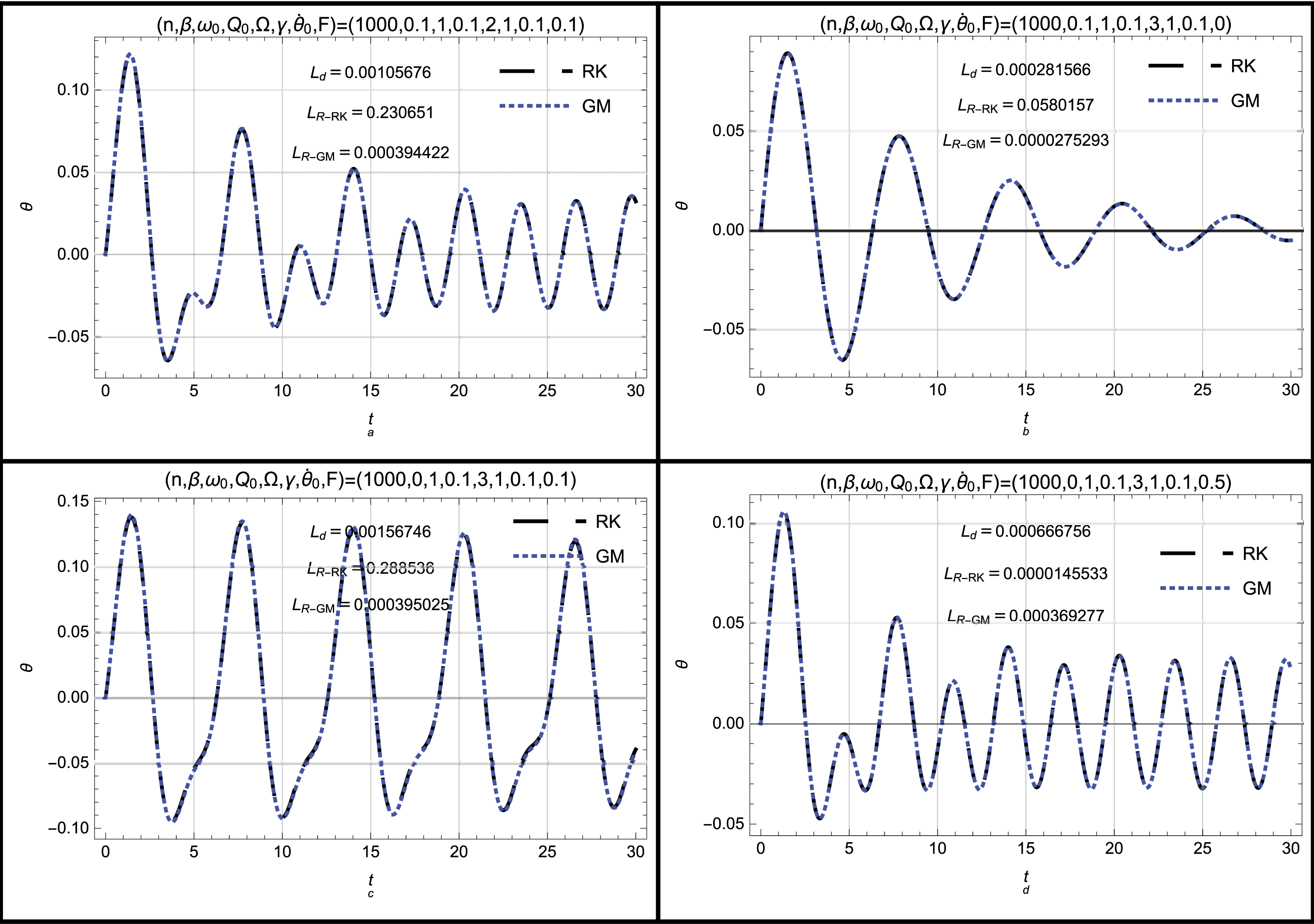
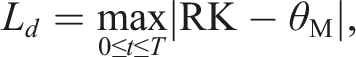
Both maximum global distance and residual errors for the numerical approximations using both GM and RK numerical method to the i.v.p. (18) are estimated for all mentioned cases.

$\left(\beta ,F,Q_0\right)$	L d	L R |RK	L R |GM
$\left(0.1,0.1,0.1\right)$	0.00105676	0.230651	0.000394422
$\left(0.1,\mathrm{0,0.1}\right)$	0.000281566	0.0580157	0.0000275293
$\left(\mathrm{0,0.1},0.1\right)$	0.00156746	0.288536	0.000395025
$\left(0.2,0.1,0\right)$	0.000666756	0.0000145533	0.000369277

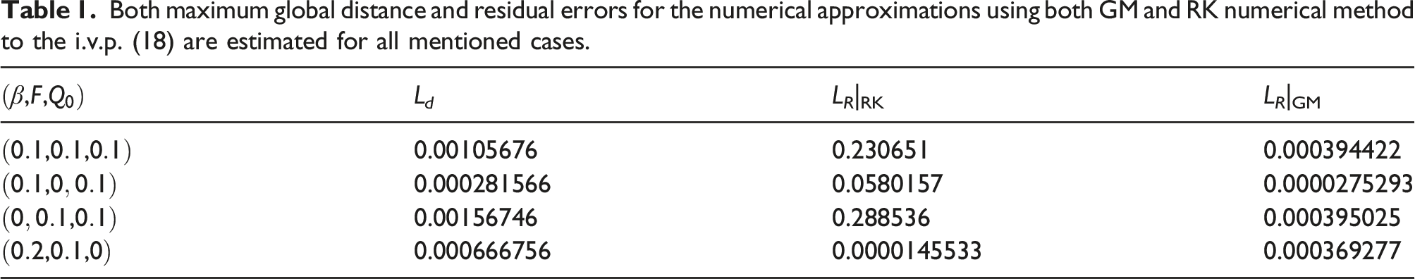
Also, all obtained numerical approximations are discussed for different values of the physical parameters $\left(n,\beta ,{\omega }_0,Q_0,\mathrm{\Omega },\gamma ,{\dot{\theta }}_0,F\right)$ . Note here that θ_M represents the approximate solution where θ_M = θ_GM, θHe′s, and θ_AM denote the Galerkin, He’s, and anzatz approximations, respectively. The impact of the hats number n on the profile of the oscillator $\theta \left(t\right)$ is studied as shown in Figure 3 at $\left(\beta ,{\omega }_0,Q_0,\mathrm{\Omega },\gamma ,{\dot{\theta }}_0,F\right)=\left(0.1,\mathrm{1,0.1},\mathrm{3,1,0.1},0.1\right)$ . Also, both maximum global distance and residual errors for different values to the hats number n are estimated in the time interval 0 ≤ t ≤ 30 as seen in Table 2.

Figure 3.

The impact of hats number n on the numerical approximations to the i.v.p. (18) using both GM and RK numerical method is investigated.

Table 2.

Both maximum global distance and residual errors for the numerical approximations using both GM and RK numerical method to the i.v.p. (18) are estimated at $\left(\beta ,{\omega }_0,Q_0,\mathrm{\Omega },\gamma ,{\dot{\theta }}_0,F\right)=\left(0.1,\mathrm{1,0.1},\mathrm{3,1,0.1},0.1\right)$

n	L d	L R |RK	L R |GM
100	0.00819291	0.230776	0.0334518
500	0.00206169	0.230776	0.0029841
1000	0.00105293	0.230776	0.000767959
2000	0.000532919	0.230776	0.000193866
104	0.000110305	0.230776	0.0000118786

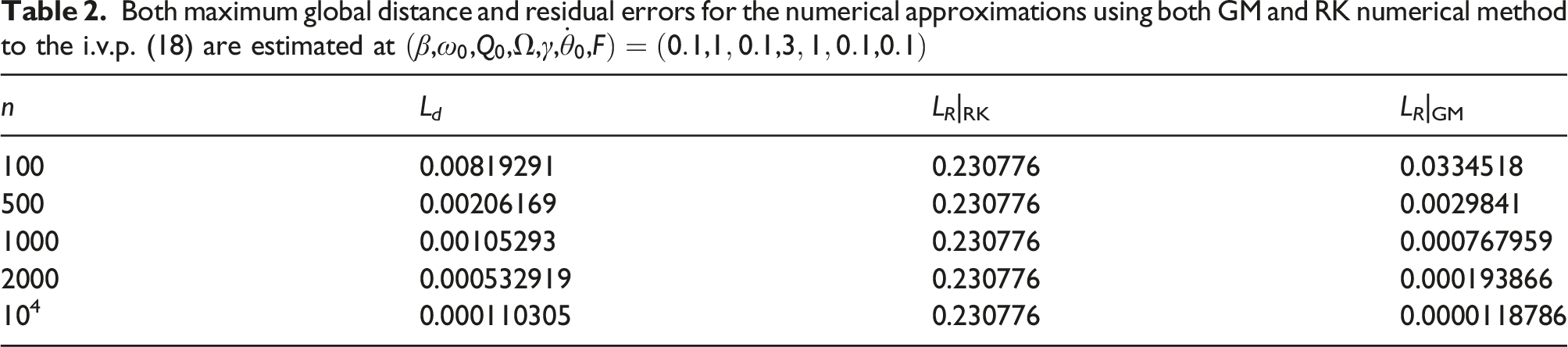
One can see that the accuracy of the approximation using GM increases with increasing the number of hats n. Also, it is clear that RK numerical approximation in this interval is not good as compared to the numerical approximation using GM. However, for long time domain say, 0 ≤ t ≤ 100 with small values to Ω, say Ω = 2 or less, the RK numerical approximation becomes better than all mentioned approximations as shown below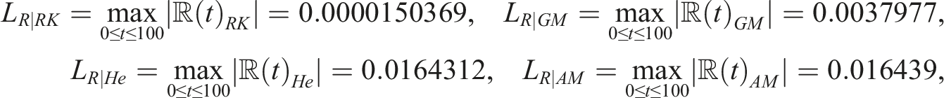

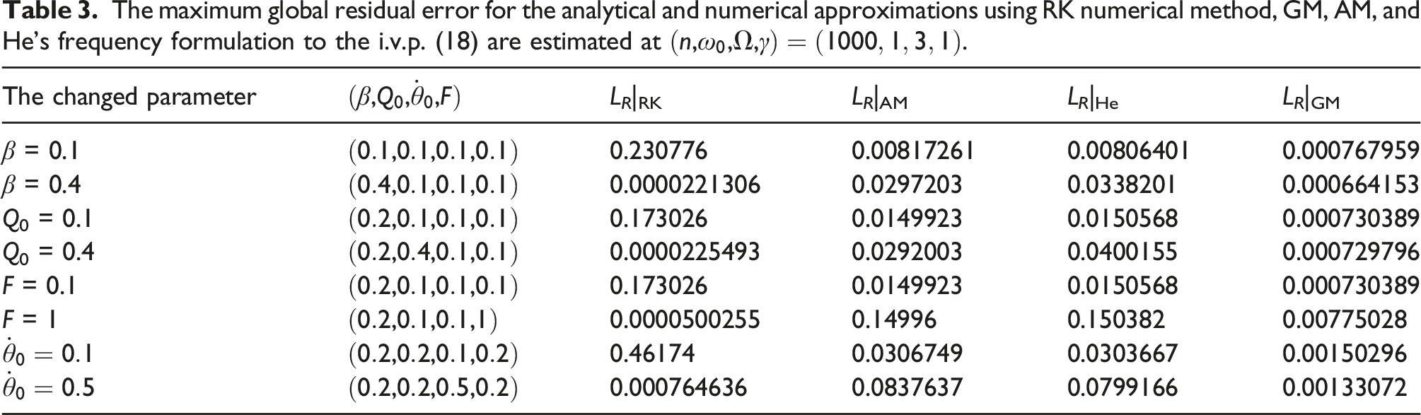
$\begin{array}{ll}{L}_{R|RK}\hfill & =\underset{0\le t\le 100}{\max }\left|ℝ{\left(t\right)}_{RK}\right|=0.0000150369,\hfill \\ L_{R|GM}\hfill & =\underset{0\le t\le 100}{\max }\left|ℝ{\left(t\right)}_{GM}\right|=0.0037977,\hfill \\ L_{R|He}\hfill & =\underset{0\le t\le 100}{\max }\left|ℝ{\left(t\right)}_{He}\right|=0.0164312,\hfill \\ L_{R|AM}\hfill & =\underset{0\le t\le 100}{\max }\left|ℝ{\left(t\right)}_{AM}\right|=0.016439,\hfill \end{array}$

here $\left(n,\beta ,{\omega }_0,Q_0,\gamma ,{\dot{\theta }}_0,F\right)=\left(\mathrm{1000,0.1},\mathrm{1,0.1},\mathrm{1,0.1},0.1\right)$ . However, the numerical approximation using GM is better than the analytical approximations using both AM and He’s frequency formulation.

For arbitrary values to the physical parameters, the effect of damping coefficient β, excitation amplitude Q₀, coefficient of forcing term F, and initial velocity ${\dot{\theta }}_0$ , on the profile of the oscillator $\theta \left(t\right)$ is investigated as illustrated in Figure 4 to 7, respectively, and at fixed values of $\left(n,{\omega }_0,\mathrm{\Omega },\gamma \right)=\left(\mathrm{1000,1,3,1}\right)$ . Moreover, the maximum global residual error is estimated for different values of the damping coefficient β, the excitation amplitude Q₀, the coefficient of forcing term F, and the initial velocity ${\stackrel{.}{\theta }}_0$ as demonstrated in Table 3 for all obtained approximations θ_M, that is, θ_M = θ_GM, θHe′s, and θ_AM denote the Galerkin, He’s, and anzatz approximations. It is clear that the GM gives stable results for arbitrary values of the physical parameters/coefficients. Moreover, this method is characterized by the high-accuracy and more stable for a long time and increasing the number of hats n leads to an increase in the accuracy of the approximations. Also, both ansatz method and He’s frequency formulation give reasonable results, but with low accuracy as compared to GM.

Figure 4.

The impact of damping coefficient β on the numerical approximations to the i.v.p. (18) using both GM and RK numerical method is investigated.

Figure 5.

The impact of excitation amplitude Q₀ on the numerical approximations to the i.v.p. (18) using both GM and RK numerical method is investigated.

Figure 6.

The impact of forcing term coefficient F on the numerical approximations to the i.v.p. (18) using both GM and RK numerical method is investigated.

Figure 7.

The impact of the initial velocity ${\dot{\theta }}_0$ on the numerical approximations to the i.v.p. (18) using both GM and RK numerical method is investigated.

Table 3.

The maximum global residual error for the analytical and numerical approximations using RK numerical method, GM, AM, and He’s frequency formulation to the i.v.p. (18) are estimated at 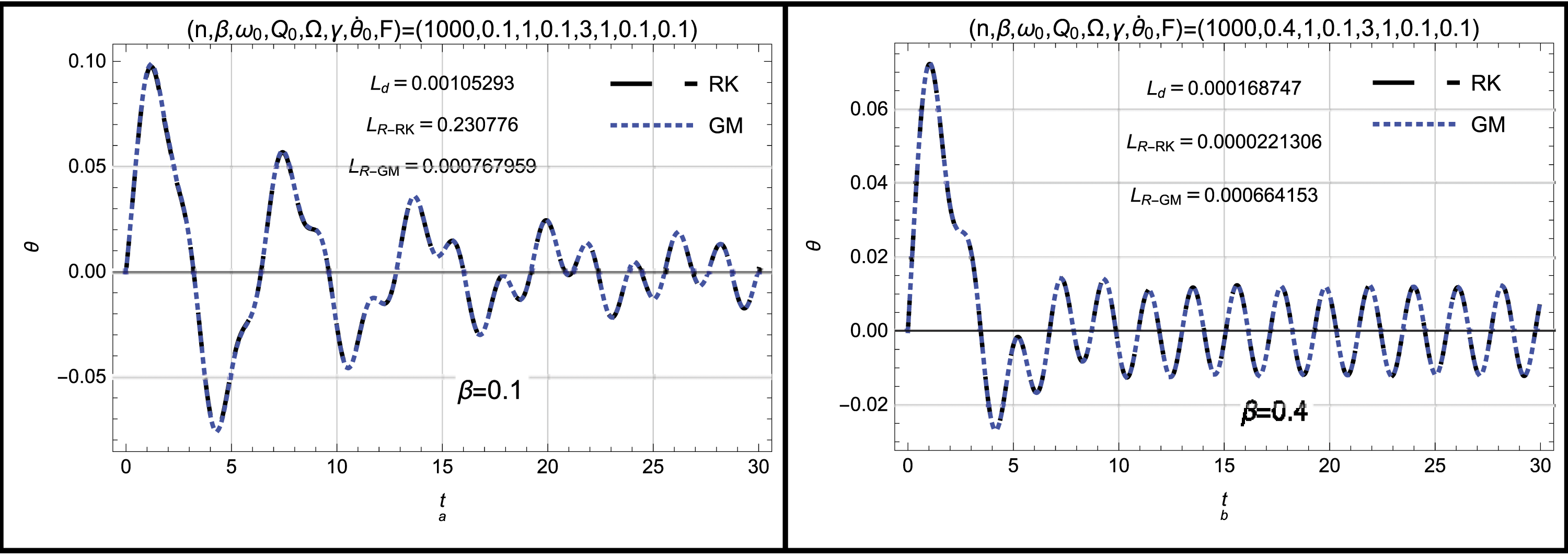$\left(n,{\omega }_0,\mathrm{\Omega },\gamma \right)=\left(\mathrm{1000,1,3,1}\right)$ .

The changed parameter	$\left(\beta ,Q_0,{\dot{\theta }}_0,F\right)$	L R |RK	L R |AM	L R |He	L R |GM
β = 0.1	$\left(0.1,0.1,0.1,0.1\right)$	0.230776	0.00817261	0.00806401	0.000767959
β = 0.4	$\left(0.4,0.1,0.1,0.1\right)$	0.0000221306	0.0297203	0.0338201	0.000664153
Q0 = 0.1	$\left(0.2,0.1,0.1,0.1\right)$	0.173026	0.0149923	0.0150568	0.000730389
Q0 = 0.4	$\left(0.2,0.4,0.1,0.1\right)$	0.0000225493	0.0292003	0.0400155	0.000729796
F = 0.1	$\left(0.2,0.1,0.1,0.1\right)$	0.173026	0.0149923	0.0150568	0.000730389
F = 1	$\left(0.2,0.1,0.1,1\right)$	0.0000500255	0.14996	0.150382	0.00775028
${\stackrel{.}{\theta }}_0=0.1$	$\left(0.2,0.2,0.1,0.2\right)$	0.46174	0.0306749	0.0303667	0.00150296
${\stackrel{.}{\theta }}_0=0.5$	$\left(0.2,0.2,0.5,0.2\right)$	0.000764636	0.0837637	0.0799166	0.00133072

Conclusions

The equation of motion of the forced damped parametric driven pendulum and some related equations have been investigated using different numerical and analytical approaches including the Galerkin method (GM), ansatz method (AM), and He’s frequency formulation. In the first, the mentioned equation of motion has been reduced to the variable-coefficients forced damped Duffing oscillator via Taylor expansion or Chebyshev approximation. After that the GM was applied for analyzing the variable-coefficients forced damped Duffing oscillator. The obtained Galerkin approximation could be recovered several cases for the pendulum oscillators. In the first case, we discussed the forced damped parametric driven pendulum oscillator/or the variable-coefficients forced damped Duffing oscillator for arbitrary velocity. Also, the unforced damped parametric driven pendulum oscillator/or the variable-coefficients unforced damped Duffing oscillator in the absence of forced term (F = 0) has been reported. Moreover, the forced undamped parametric driven pendulum oscillator/or the variable-coefficients forced undamped Duffing oscillator in the absence of damping term (β = 0) has been investigated. Furthermore, we studied the forced damped parametric pendulum oscillator/or the constant-coefficients forced damped Duffing oscillator in the absence of driven term (Q₀ = 0). On the other side, some analytical approximations to all mentioned evolution equations have been derived in detail via both ansatz method and He’s frequency formulation.

The numerical approximations using GM and the analytical approximations using AM and He’s frequency formulation have been discussed and compared with the RK numerical approximations. It was observed that the numerical approximations using GM give high-accurate results as compared to the RK numerical approximations and the analytical approximations, and this is one of the most important features of the GM. Thus, this method is considered one of the powerful and effective numerical methods for solving dynamic problems due to its high-accuracy. All used methods and obtained approximations can help many researchers in modeling and analyzing nonlinear oscillations in different plasma models.