Sage Journals: Discover world-class research

Abstract

This study presents a fault diagnosis system for vehicle heating, ventilation and air conditioning (HVAC) acoustic signal with various feature extractions in deep learning neural network. Traditionally, sound used for fault diagnosis or signal classification is observed the difference of energy in time or frequency domains. Unfortunately, the frequency smearing effect often arises in some critical conditions. In the present study, discrete wavelet transform (DWT) and wavelet packet transform (WPT) are proposed in fault diagnosis. Meanwhile, when using mechanical learning methods, the data are relatively large, in order to reduce the amount of data, DWT and WPT low-frequency decomposition could be used to improve the performance. Furthermore, the signal characteristics more comprehensive, this study attempts to use the feature extraction method of wavelet packet conversion to improve the signal characteristics. In the experiment process, the operation state of the blade blower in the vehicle air conditioner, four different faults were designed, test database was established through sound to classify, and identify the data using deep neural networks to achieve the purpose of blower fault diagnosis. In data analysis, the original signal is presented through wavelet packet decomposition and discrete packet conversion technology, compared with traditional time and frequency domain signals to explore the identification rate, identification speed and related issues. Experimental results show that using WPT combined with deep neural networks have good fault diagnosis and discrimination capabilities, training, and identification time is shorter than time-frequency domain signals.

Keywords

Feature extraction discrete wavelet transform wavelet packet transformation deep neural network fault diagnosis

Introduction

The vehicle heating, ventilation, and air conditioning (HVAC) system is an important system for vehicle comfort, however, people often ignore the maintenance of the air-conditioning part, and they will realize that the system is damaged when there is a real failure. This study uses the vehicle fault sound on the air-conditioning blower allows the driver to detect the problem early and avoid expanding blower damage. This research mainly uses the methods of deep learning and machine learning to establish a set of fault diagnosis identification system using the sound of vehicle air conditioner blowers. As early as the 1960s, information scientists were inspired by biological nervous systems and proposed multi-level neural networks hope that by simulating the biological nervous system, computers can achieve high intelligence like humans. But immediately encountered two serious problems. The first is the lack of computing power of the computer hardware equipment at the time, which could not be applied immediately. The second is that it was not easy to obtain a large amount of data, computers cannot train and learn, so that the neural network-like has not been dazzling performance. In the recent years, computer hardware and technology have continued to advance, and it has become much easier to obtain a large amount of data. When computers can use data to quickly train and learn, can be applied to science and technology, machine learning and deep learning have once again attracted attention.

In 2014, Gencoglu et al.¹ proposed the use of deep neural networks (DNN) to identify isolated sound events such as footsteps, baby crying, motorcycle, and rain. For the task of sound event classification with 61 different classes, the experimental results prove that the classification performance of DNN is much better than traditional audio classifiers using Hidden Markov model (HMM) and Gaussian mixture model (GMM) in the same database. In 2016, Kim et al.² proposed a new method for automatic modulation classification based on DNN. The method uses 21 features extracted from DNN baseband signal samples, using DNN to classify five modulation formats. Simulations performed under various conditions show that deep neural networks are faster than artificial neural network (ANN) classifiers with shallow structures. In 2019, Huang et al.³ proposed the Laplacian score-deep belief network (LS-DBN) based on a novel intelligent acoustic model based on DNN to evaluate the sound quality of EV interior noise. The interior noises of 10 EVs were recorded on eight different road surfaces. The results show that the proposed LS-DBN model is superior to the conventional DBN and BPNN in terms of accuracy and stability, and it is highly efficient. In the same year, Huang et al.⁴ proposed a novel method to use the original time signals and frequency spectra for identifying and predicting EV shock absorber squeak noise based on DNN. An EV road test is conducted on five different pavements. The DNN outperforms the genetic algorithm-back propagation neural network (GA-BPNN) and the genetic algorithm-support vector machine (GA-SVM), based on a confusion matrix and an error analysis. In addition, deep learning has more excellent effects than traditional classifiers.

In order to improve the classification recognition rate, signal conversion and feature extraction are very important. The fast Fourier transform (FFT) ⁵ is used for the conversion. The domain signal is converted into a frequency domain signal, which is helpful for signal analysis and allows researchers to know the frequency of the sound more clearly. Although the Fourier transform makes the signal clearer, it improves the recognition rate of system fault diagnosis but cannot reduce the data in the database, which makes the classifier take more time to identify.

In order to improve the problem of huge data sets, discrete wavelet transform (DWT) is used as the method of analyzing noise. The main structure of discrete wavelet is composed of a pair of low-frequency filters and high-frequency filters, the low-frequency parts are continuously decomposed to reach multiple layers. The function of analysis makes the signal characteristic value easy to be extracted and greatly reduces the data in the database .^6–8 However, only the low frequency is decomposed to make the signal characteristic value not comprehensive enough. To improve the problem that the characteristic value is not complete, wavelet packet transformation (WPT) is used as a method for analyzing noise. The structure of wavelet Packet transformation is the same as discrete wavelet transformation, but WPT not only decomposes low frequencies, but also decomposes high frequencies to extract eigenvalues, which can not only reduce the amount of data, but also make the signal characteristic more complete. In recent year, Ehya et al.⁹ proposed the use of discrete wavelet transform and more different signal processing tools to diagnose the faults of hydrogenerators operating, with a central focus on additive noise impacts on processed data. Mathew et al.¹⁰ proposed the use of WPT, principle component analysis and bayesian optimization to evaluate engine faults. The two literatures both demonstrated improved accuracy and the performance metrics.

Principle of noise feature extraction and deep neural network

Discrete wavelet transform

The traditional signal analysis mainly uses Fourier transform. Fourier transform is an important algorithm for digital signal processing. However, the common signals are continuous and non-periodic, after conversion, it becomes continuous and aperiodic in the frequency domain. Both of the time domain and frequency domain are continuous signals, which makes it difficult for computers to calculate and process. Therefore, using discrete Fourier transform (DFT),¹¹ a one-to-one function is used to decompose a complex wave into waves composed of N sin and N cos (from 0 times to N-1 times). Add the frequencies, amplitudes, and phases of different waveforms together so that the time and frequency domains are discrete and can be calculated by computer, as shown in equation (1).

X (k) = \sum_{n = 0}^{N - 1} x (n) ˙ e^{- \frac{i 2 π k n}{N}} (0 \leq k \leq N - 1)

(1)

Although DFT solves the problem of computer calculation, if DFT signal is used for calculation, the amount of data is large and the calculation speed is slow. Therefore, this study uses FFT as the feature extraction method. FFT uses DFT as The basic extension, but the FFT can greatly reduce the calculation time.

After the sound signal is converted from the time domain to the frequency domain, although the characteristics of the signal can be polished in the frequency domain, the change of the time-cut frequency cannot be converted. Therefore, many scholars have proposed continuous wavelet transform (CWT) to improve Fourier transform.¹² When the a value is aligned, the wavelet is transformed to expand, while more a values are broken and compressed, and the m value is used as the best step of the wavelet on the time axis. For the effect of distance, when the wavelet is narrow, choose a smaller value of m. If the wavelet is wider, choose the value of m. The CWT algorithm is shown in equation (2).

CWT (a, m) = \frac{1}{\sqrt{a}} \int_{- \infty}^{\infty} x (t) ψ (\frac{t - m}{a}) d t

(2)

CWT calculates the signal at every possible scale to obtain the converted wavelet coefficients. Such a calculation process will cause a huge amount of data. Therefore, in order to reduce the huge calculation amount of CWT, DWT was developed.^13-15 DWT discretizes the scale parameter a and translation parameter m in the CWT formula by 2n. The DWT algorithm is shown in equation (3).

DWT (a, n) = \frac{1}{\sqrt{2^{j}}} \int_{- \infty}^{\infty} x (t) ψ (\frac{t - 2^{j} k}{2^{j}}) d t

(3)

The scale parameter of a is 2j, the translation parameter of n is 2 ^ j k, n is the number of layers for signal decomposition. In this way, the analysis scale and data volume can be greatly reduced.

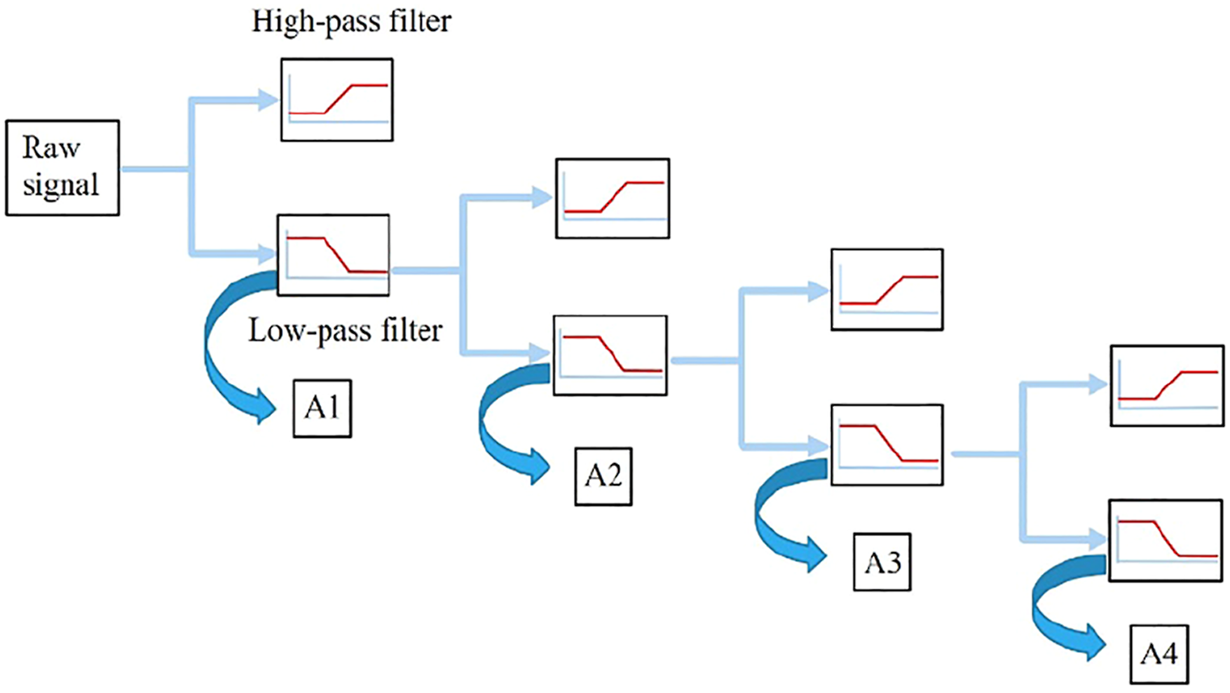
DWT can be regarded as multi-resolution decomposition. The signal is sent to a high-pass filter and a low-pass filter. After the signal enters the high-pass and low-pass filters, and then the sample is reduced by half, the high-frequency wavelet and the coefficients of the low-frequency wavelet are shown in Figure 1, and then decomposed by the value of the low-pass filter. After the layer-by-layer decomposition, the characteristic values of the wavelet are obtained. As shown in Figure 2, it will be decomposed. The main reason is that for most signals, low frequency is often important. If the high frequency of the signal is removed, the characteristic value of the signal can still be retained. It is an approximation after being decomposed by a low-pass filter; it is a detail after being decomposed by a high-pass filter.

Figure 1.

Signal filtering decomposition.

Figure 2.

Principle of discrete wavelet transform.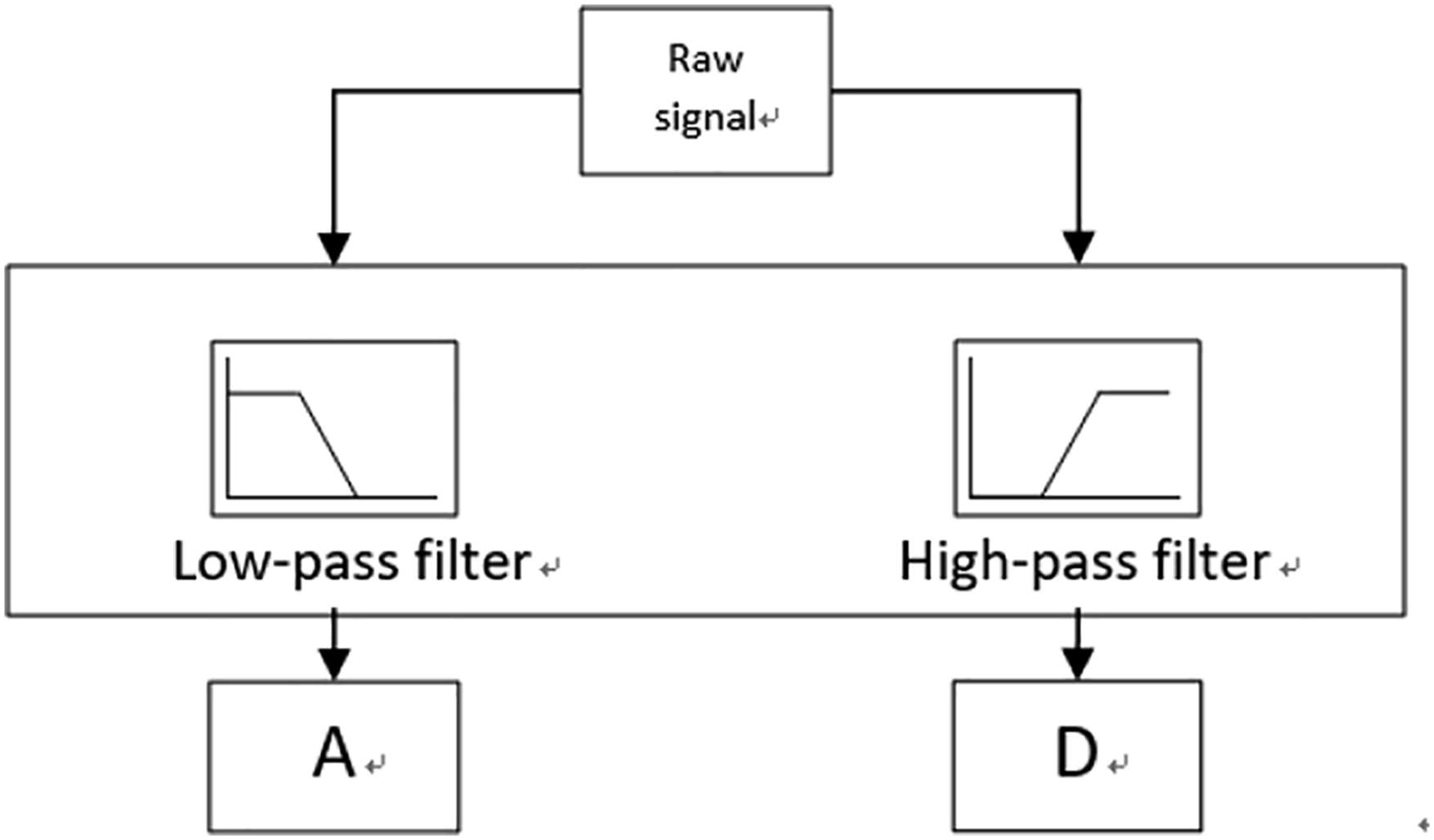

Wavelet packet decomposition

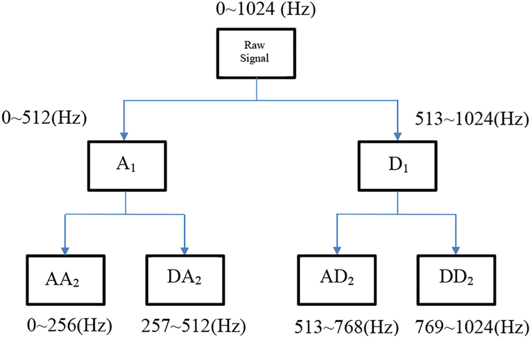
Although the DWT has greatly reduced the amount of data, it only decomposes the low frequency, the high frequency part of the signal no longer continues to be decomposed. Therefore, the DWT can express the main characteristics of the low frequency, but cannot fully decompose the signal. The principle of wavelet transformation is basically the same as that of WPT. Both decompose the original signal into high frequency and low frequency, but WPT can decompose the noise signal more comprehensively.^16–18 It can decompose both the low frequency part and the high frequency part as shown in Figure 3. The frequency part is decomposed to make the signal decomposition more comprehensive, so that signals containing medium and high frequencies can be better analyzed locally. The wavelet packet representation function is Ψ, i is the modulation parameter, j is the scaling parameter, k is the translation. The parameters are shown in equation (4).

ψ_{j, k}^{i} (t) = 2^{- \frac{j}{2}} ψ^{i} (2^{- j} t - k)

(4)

where i is the number of layers of wavelet packet tree decomposition,¹⁹ the wavelet is obtained through the following recursive relationship, as shown in equations (5) and (6).

ψ^{2 i} (t) = 1^{- \frac{1}{2}} \sum_{k = - \infty}^{\infty} h (k) ψ^{i} (\frac{t}{2} - k)

(5)

ψ^{2 i + 1} (t) = 1^{- \frac{1}{2}} \sum_{k = - \infty}^{\infty} g (k) ψ^{i} (\frac{t}{2} - k)

(6)

Figure 3.

Principle of wavelet packet decomposition.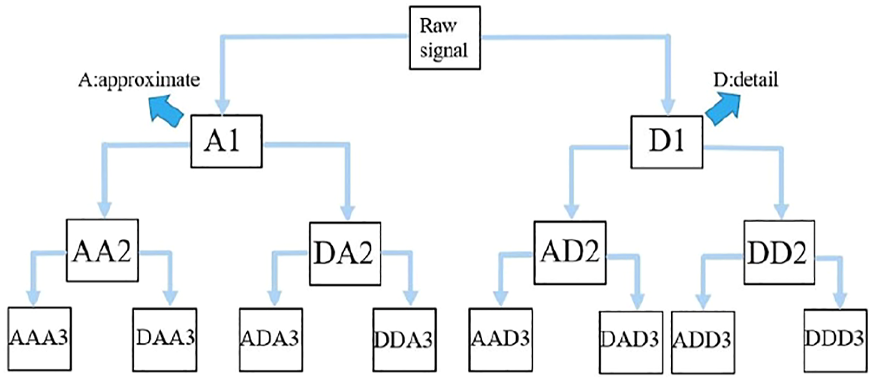

The discrete filters h (k) and g (k) are orthogonal mirror filters associated with the scaling function and the mother wavelet function, the two filters h (k) and g (k) are also called group conjugate orthogonal filter.

The wavelet packet coefficient C corresponding to the signal f (t) can be obtained as shown in equation (7).

C_{j, k}^{i} = \int_{- \infty}^{\infty} f (t) ψ_{j, k}^{i} (t) d t

(7)

Assuming the wavelet coefficients meet the conditions of intersection, the WPT of the signal at a specific node can be obtained as shown in equation (8).

f_{j}^{i} (t) = \sum_{k = - \infty}^{\infty} C_{j, k}^{i} ψ_{j, k}^{i} (t) d t

(8)

After performing WPT to the n stage, the original signal can be expressed as the sum of all wavelet packet components of the n stage, as shown in equation (9). The structure composed of low-pass and high-pass filters is used in the restructure filter bank.

f (t) = \sum_{i = 1}^{2 i} f_{j}^{i} (t)

(9)

Structure of deep learning neural network

Deep learning is a new research direction in the field of machine learning. In the early days, information scientists were inspired by biological neural network systems and proposed multi-level artificial neural networks (ANN).²⁰ It is hoped that by simulating the biological nervous system, the computer can also achieve high intelligence like humans, but it was limited by the computing power of the computer at the time and a large number of digital data was difficult to obtain, so that the neural network-like has no amazing effect, but with the advancement of computer hardware in recent years, machine learning introduced with deep learning can be closer to artificial intelligence. Compared with traditional neural networks, deep learning contains more hidden layers. Machine learning implements a feedforward artificial neural network, more specifically called a multilayer perceptron (MLP).²¹ It consists of input, output, and a or multiple hidden layers, each layer includes one or more neurons connected to the previous and next layer neurons, all neurons of the MLP are similar, each of them has several input keys that take the output values of several neurons in the previous layer as inputs and input them into several outputs, and then pass the response to several neurons in the next layer. In the middle of building a model, in addition to input and output, the number of hidden layers and the weight value of neurons will affect the result.

The difference between predicted and actual output is expressed as cost function, also sometimes referred as loss function. The actual value and back-propagate (BP) the error from the output layer to the hidden layer.²² BP is short for error back propagation and is used in combination with the gradient descent method,²³ which is an ANN training method. This gradient calculates the weight loss function in the network and feedback to the optimal method to update the weights to minimize the loss function. Deep learning is to stack several hidden layers, as shown in Figure 4, which makes the neuron’s computing weight larger, the judgment is more accurate, the recognition rate is higher.

Figure 4.

Principle of deep neural network.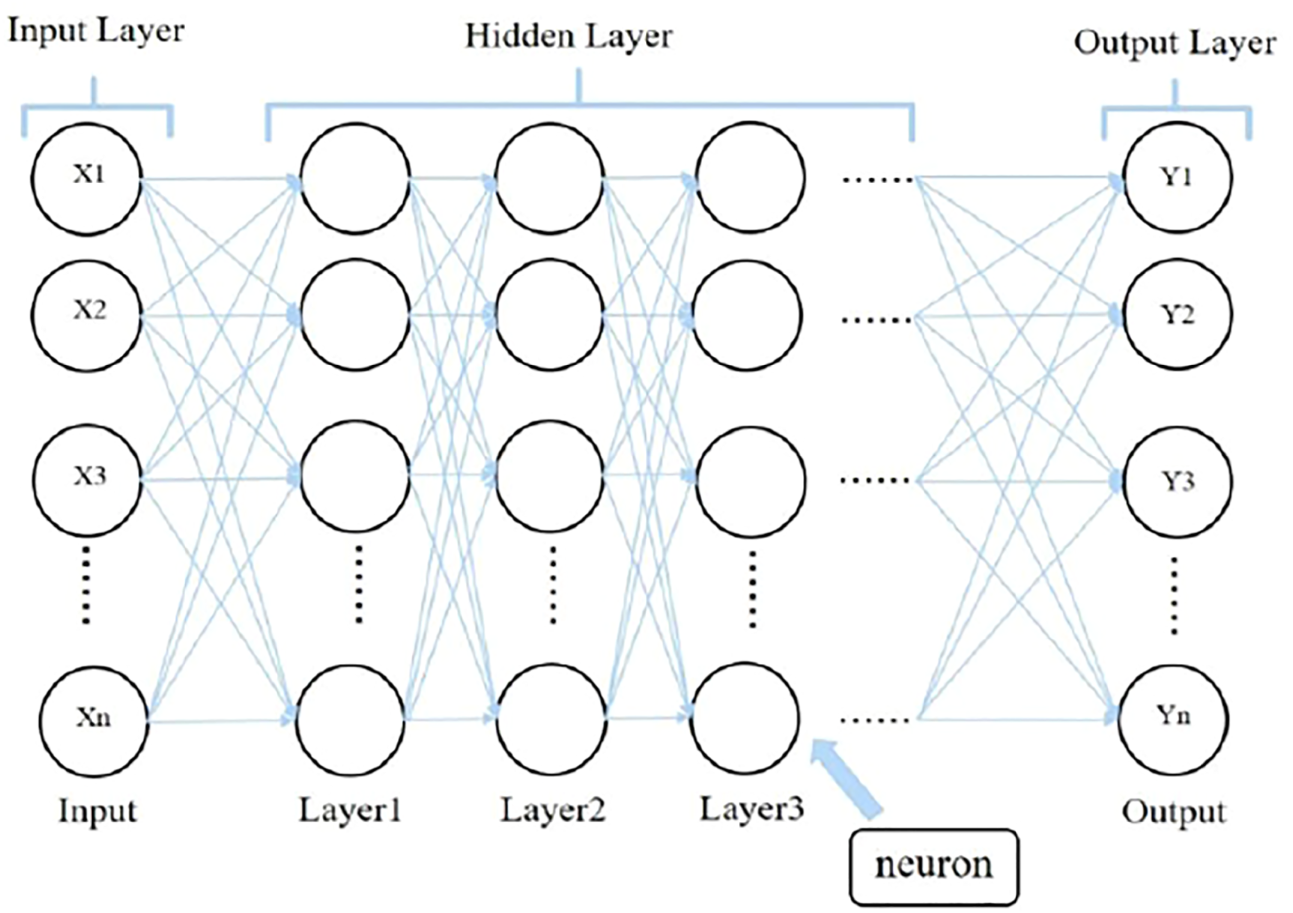

Learning framework

Deep learning models are large and complex. If we handcode it from scratch, it takes a lot of time. For this reason we use frameworks and software libraries to accelerate the coding part to build neural networks. In the present study, tensorflow as the framework²⁴ is used. Tensorflow will be used for several reasons, Tensorflow was developed by Google, Google is not only a leader in big data, but also has a good practices in machine learning and deep learning, compared with other frameworks, tensorflow has faster compilation speed, it is the most complete in open source resources, it can design neural network structures by itself. It has rich applications in audio processing, graphic classification and natural language applications. The above reasons make tensorflow the most popular framework choice.

Python language

The topics of machine learning and deep learning that have been used in recent years have made python,²⁵ the most commonly used programming language for engineers for the following reasons. Python has simplified a lot of unnecessary semicolons and brackets, most computer programming languages are compiled, the source code needs to be compiled into an executable binary format before execution. Compiling large projects can be very time consuming. The python language used in the research can execute programs directly from the source code, and it does not need to be compiled into binary code. Data analysis, engineering, and scientific functions can be used, such as Pandas and Numpy for data processing, Scikit-Learn for machine learning and Matplotlib, which can visually draw data, etc. All sorts, this research uses python as the compiler. The package used in this study is Anaconda,²⁶ and the environment is compiled with spyder.

Implementation and experimental work of blower fault diagnosis

Experimental work and data measurement

This experiment uses the air-conditioning blower of the NISSAN TEANA car, which includes the blower motor, fan blades, and air hood. The blower is placed in an environment with sound-absorbing cotton as our experimental platform. The microphone is used to measure the sound and then the data is retrieved. The analog signal received by the data acquisition is converted into a digital signal by software and stored on the computer. The sound capture process is shown in Figure 5. A variety of fault conditions were set in this experiment: A. normal, B. hosing flapping, C. blade damaged, D. leaves in the blower, and E. bearing lubrication failure. The sampling frequency for sound measurement in 2048 Hz, the number of sampling points is 20,480, and the sampling time is 10 s. In each fault condition, five kinds of speeds are simulated, which are 300 rpm, 600 rpm, 900 rpm, 1200 rpm, and 1500 rpm. There are 25 conditions in total, each of which measures 20 sound signals.

Figure 5.

Experimental setup and process.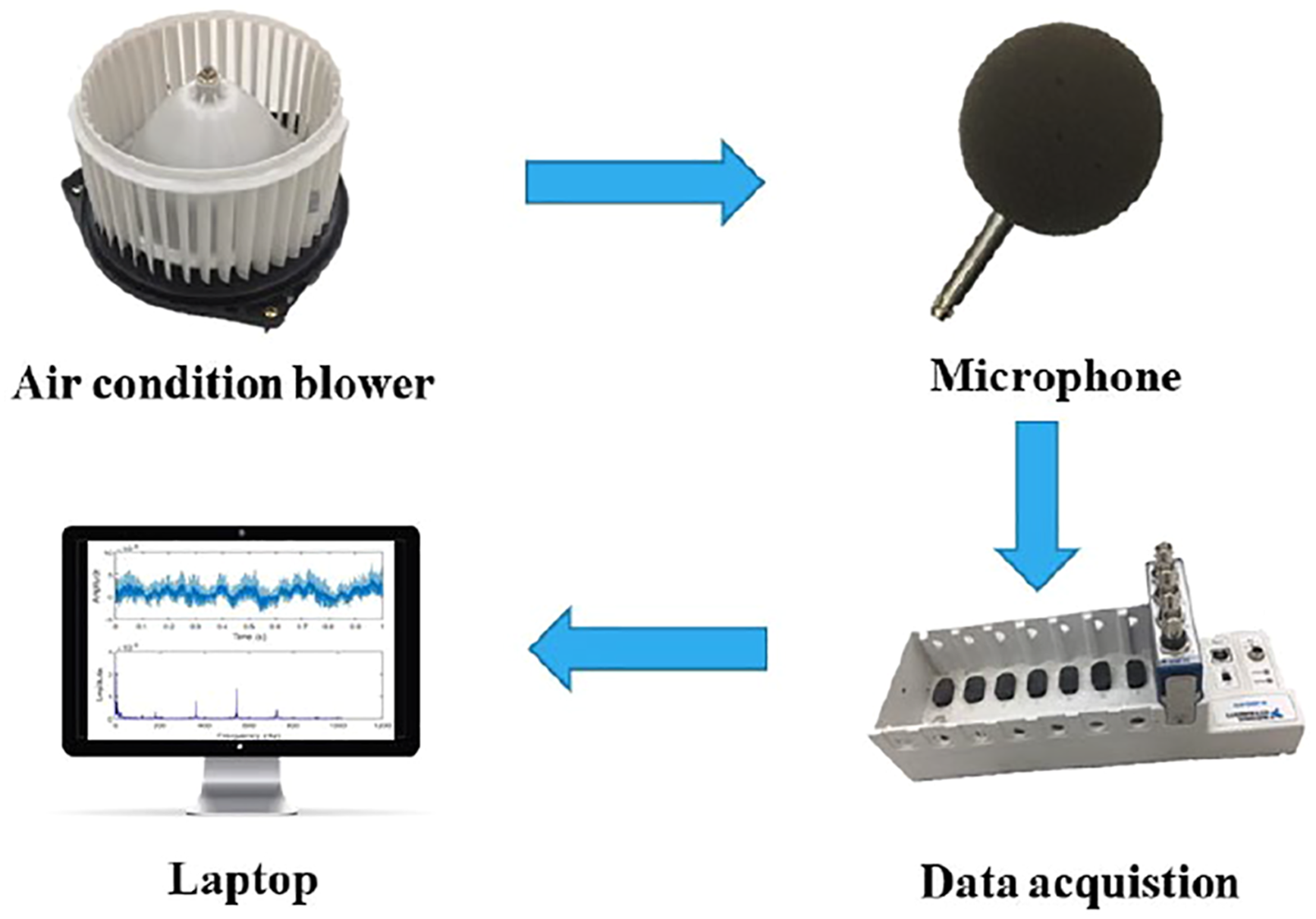

Blade blower sound signal processing

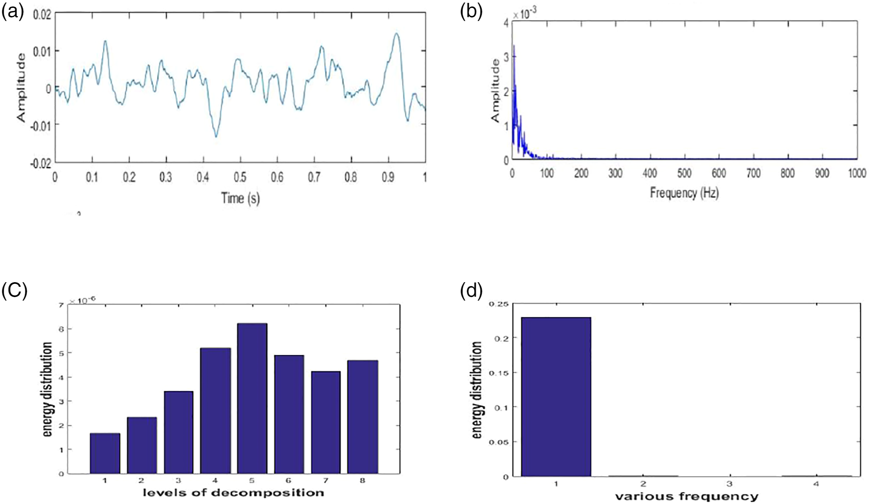
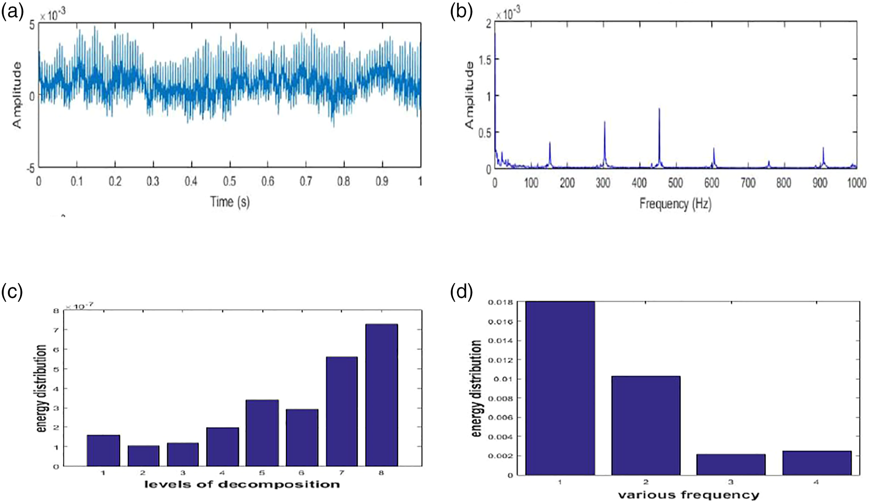
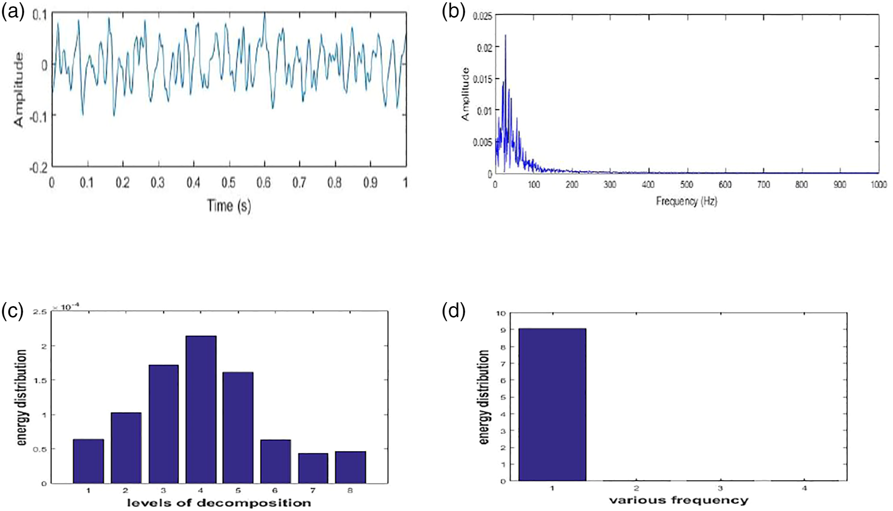
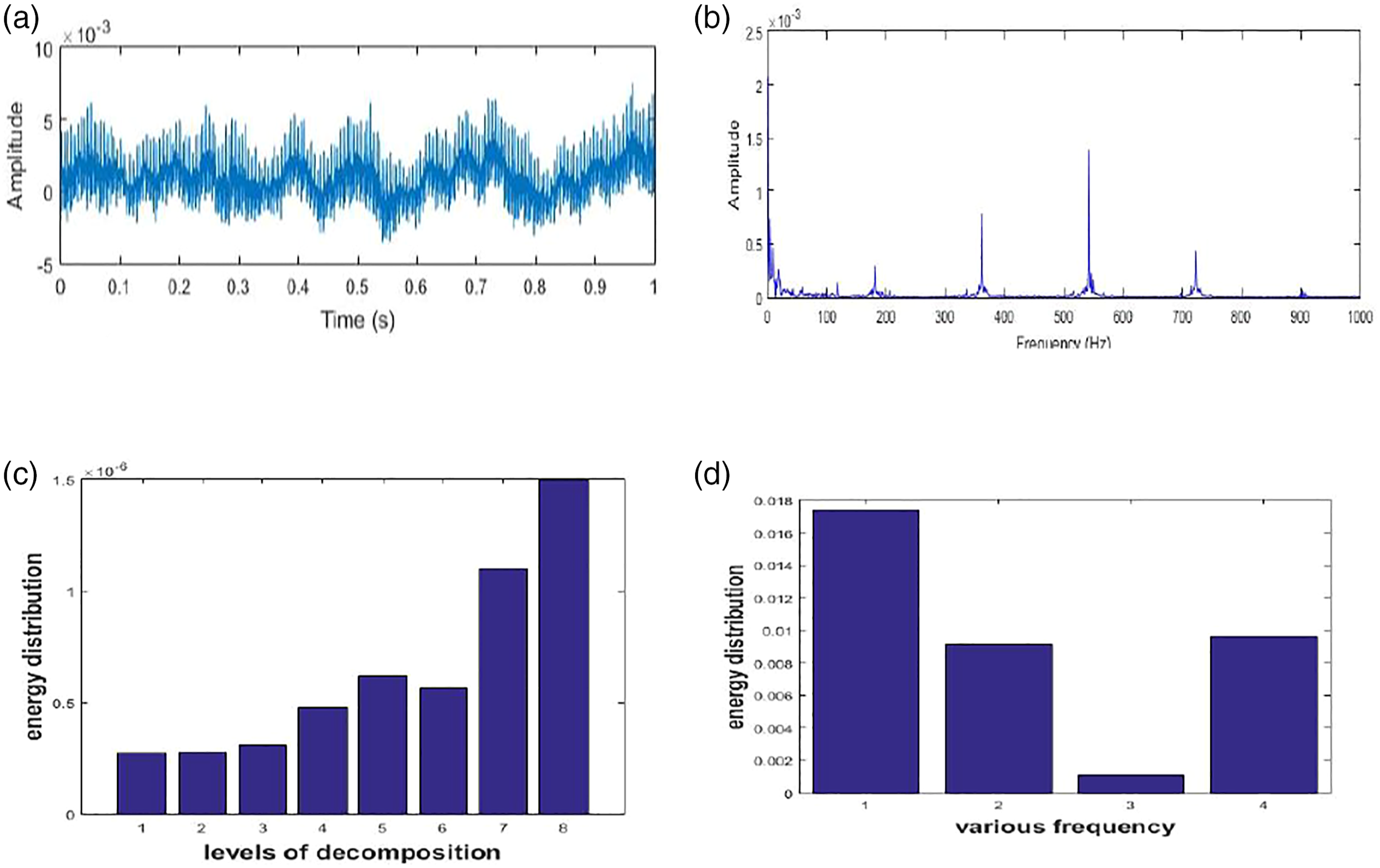
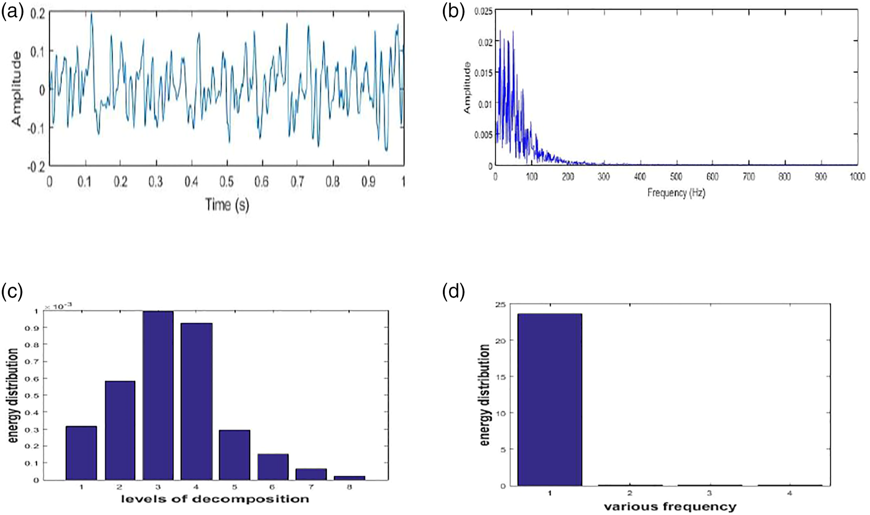
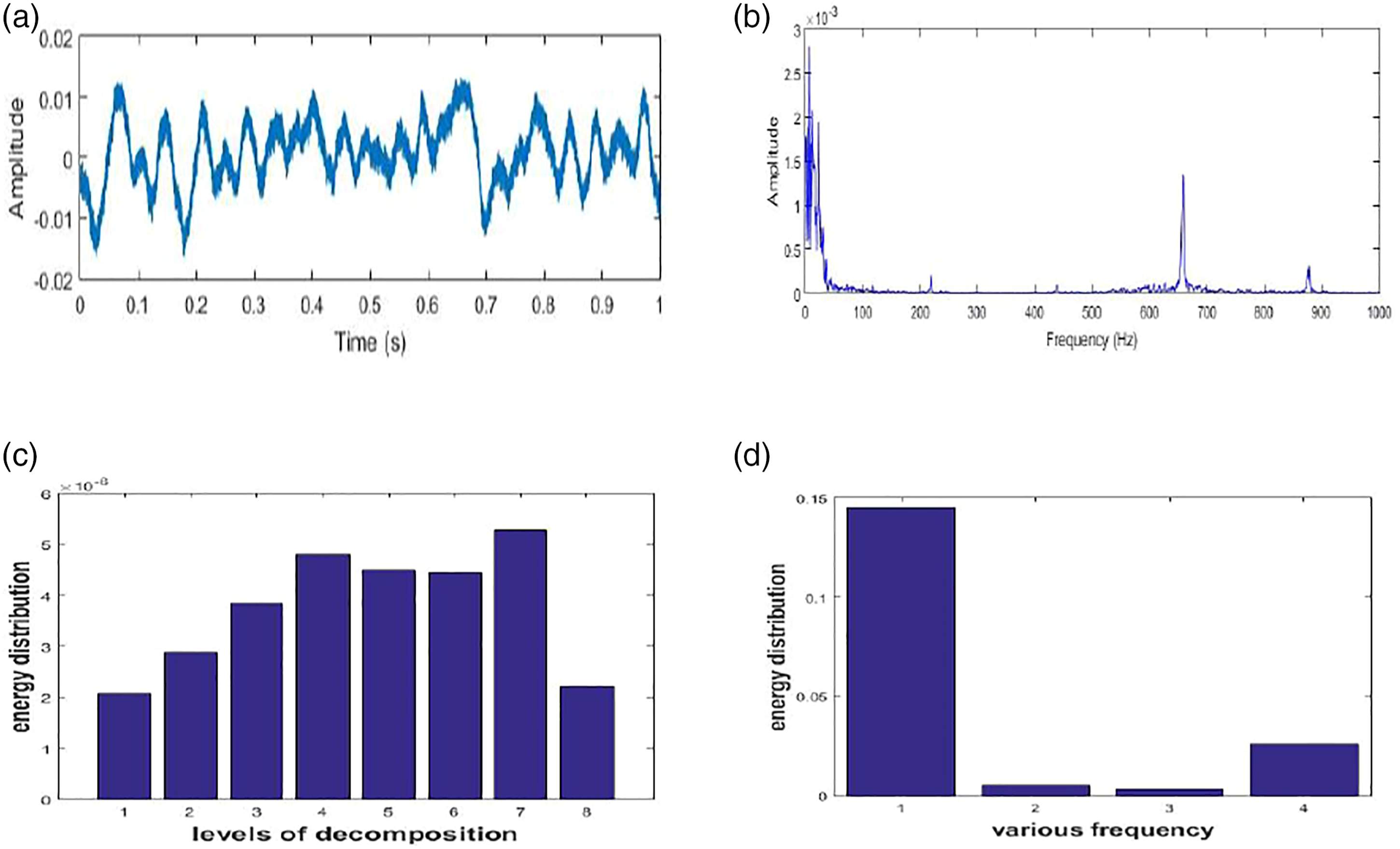
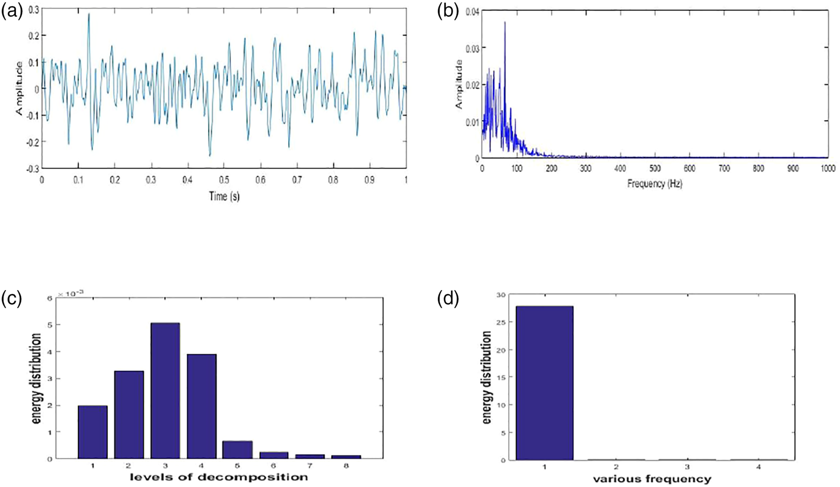
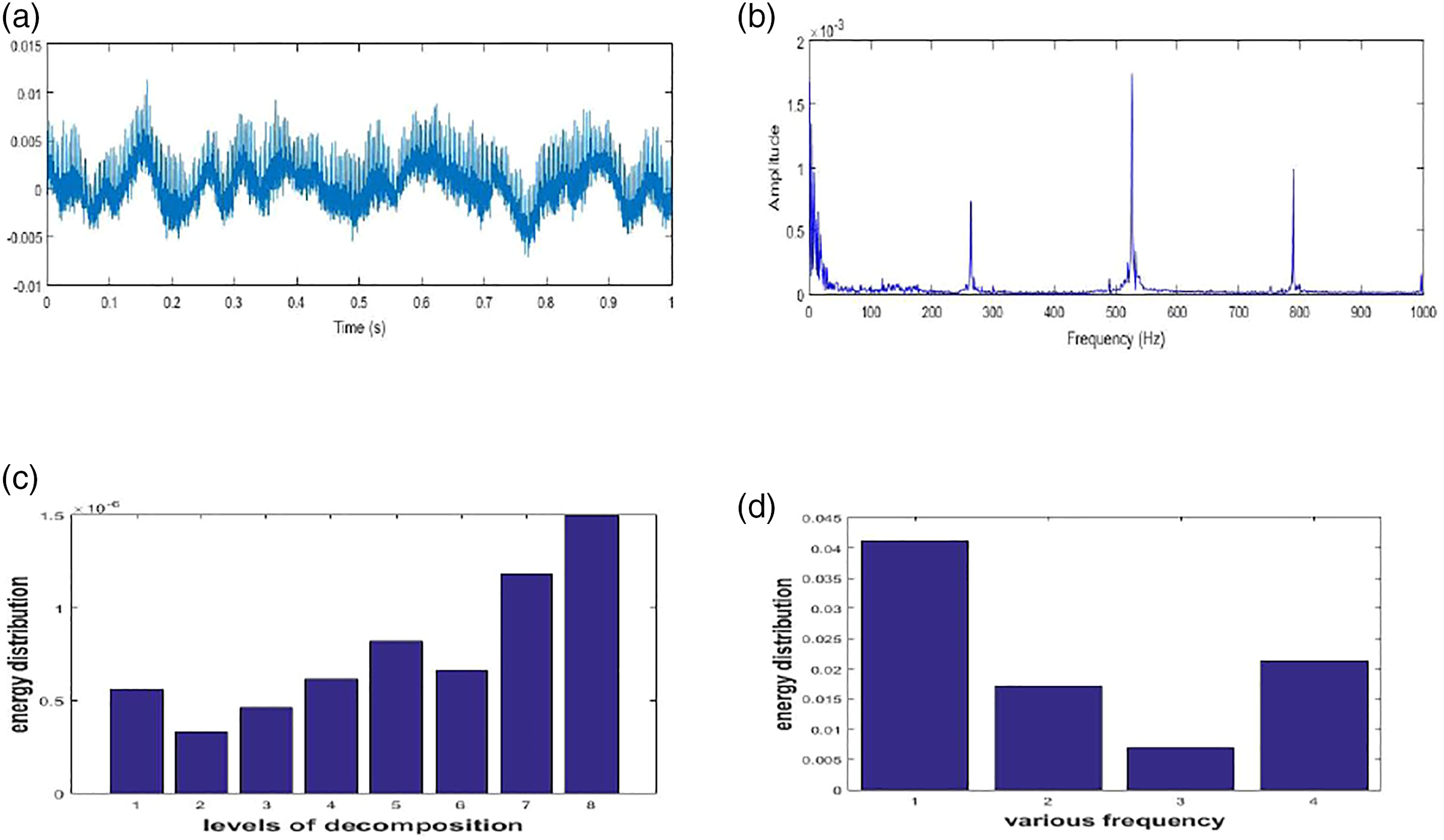
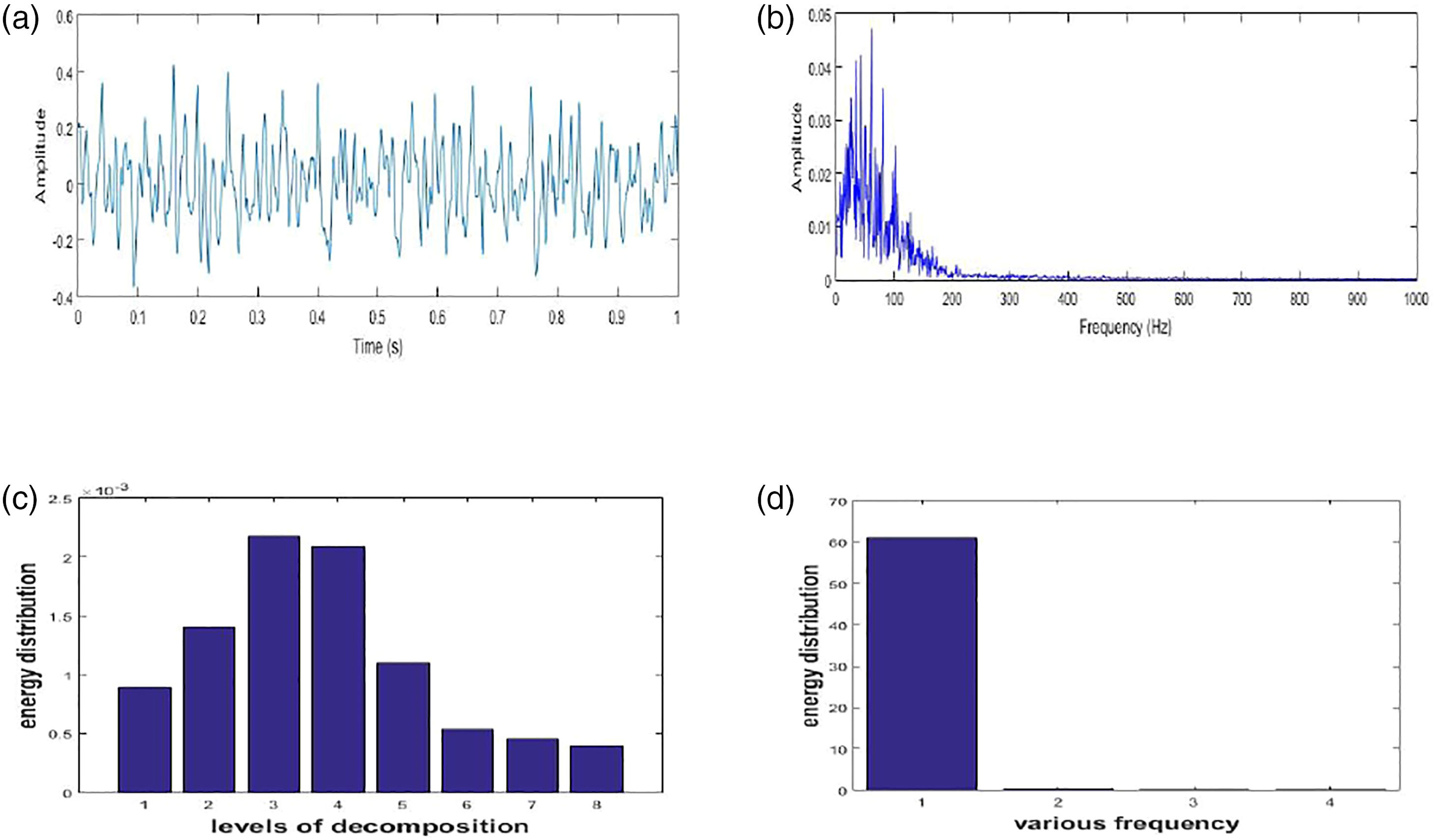
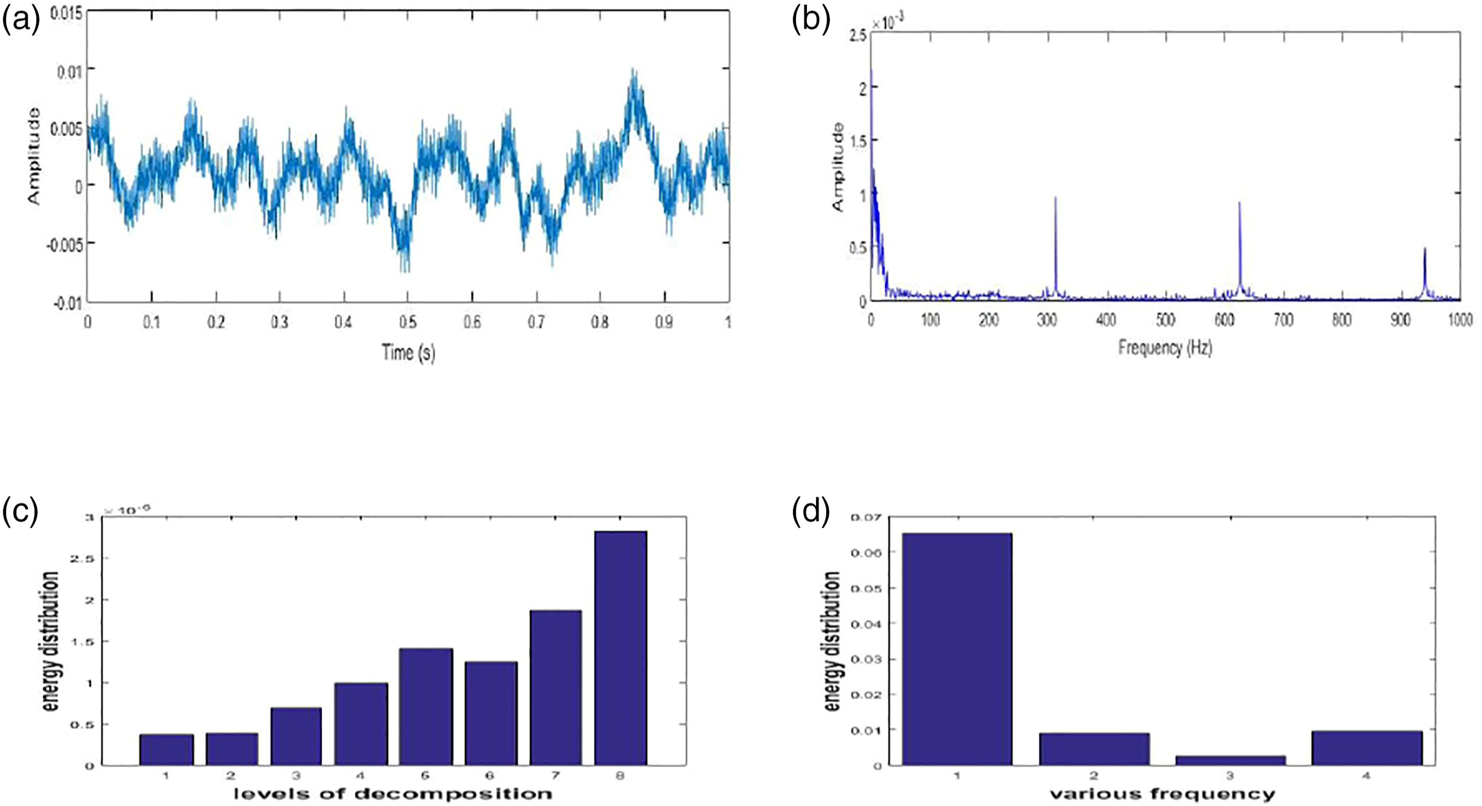
Five speeds were recorded in the experiment and five blower failures were simulated. A total of 25 kinds of original signal files were used. The first feature extraction method was used to convert the time domain of the original signal into a signal in the frequency domain. The second feature extraction method is DWT. The time domain signal serves as an input into the DWT for feature extraction. The time domain is decomposed into seven layers through low frequency, as shown in Figure 6. WPT is used as the third feature extraction, using time domain signals to feed into WPT. Unlike DWT, which only decomposes low frequencies, WPT also decomposes high frequencies. The original signal is decomposed into high and low frequency signals. The signal has four frequency ranges. The characteristic values of AA2 + DA2 + AD2 + DD2 will be equal to the original signal. As shown in Figure 7, the characteristic values of high and low frequency signals are obtained. Then, the time domain, frequency domain, DWT, and WPT are sent to the system respectively for deep learning classification identification. The classification used three stacked hidden layers for training. The cell size of each hidden layer was set as 5 classes*10, 5 classes*20, and 5 classes*10, respectively. The signals used in the DNN contained 4096 features per time domain sample, 2048 features per frequency domain sample, eight features per DWT sample, and four features per WPT sample. An adaptive gradient algorithm which has been called Adagrad was used as the optimizer. The ReLU function was used as the activation function for the layers. In the last layer, a softmax function was used to classify. The experimental diagrams of the normal and housing flapping original signals that entered the above four experiments are shown in the Figures 8–17. The identification rate of blower fault diagnosis is obtained.

Figure 6.

Frequency distribution of Discrete Wavelet Transform in experiments.

Figure 7.

Frequency distribution of Wavelet Packet Transform in experiments.

Figure 8.

Different features are captured at normal blower in 300 rpm: (a) time domain, (b) frequency domain, (c) DWT domain, and (d) WPT domain.

Figure 9.

Different features are captured at blower of housing flapping in 300 rpm: (a) time domain, (b) frequency domain, (c) DWT domain, and (d) WPT domain.

Figure 10.

Different features are captured at normal blower in 600 rpm: (a) time domain, (b) frequency domain, (c) DWT domain, and (d) WPT domain.

Figure 11.

Different features are captured at blower of housing flapping in 600 rpm: (a) time domain, (b) frequency domain, (c) DWT domain, and (d) WPT domain.

Figure 12.

Different features are captured at normal blower in 900 rpm: (a) time domain, (b) frequency domain, (c) DWT domain, and (d) WPT domain.

Figure 13.

Different features are captured at blower of housing flapping in 900 rpm: (a) time domain, (b) frequency domain, (c) DWT domain, and (d) WPT domain.

Figure 14.

Different features are captured at normal blower in 1200 rpm: (a) time domain, (b) frequency domain, (c) DWT domain, and (d) WPT domain.

Figure 15.

Different features are captured at blower of housing flapping in 1200 rpm: (a) time domain, (b) frequency domain, (c) DWT domain, and (d) WPT domain.

Figure 16.

Different features are captured at normal blower in 1500 rpm: (a) time domain, (b) frequency domain, (c) DWT domain, and (d) WPT domain.

Figure 17.

Different features are captured at blower of housing flapping in 1500 rpm: (a) time domain, (b) frequency domain, (c) DWT domain, and (d) WPT domain.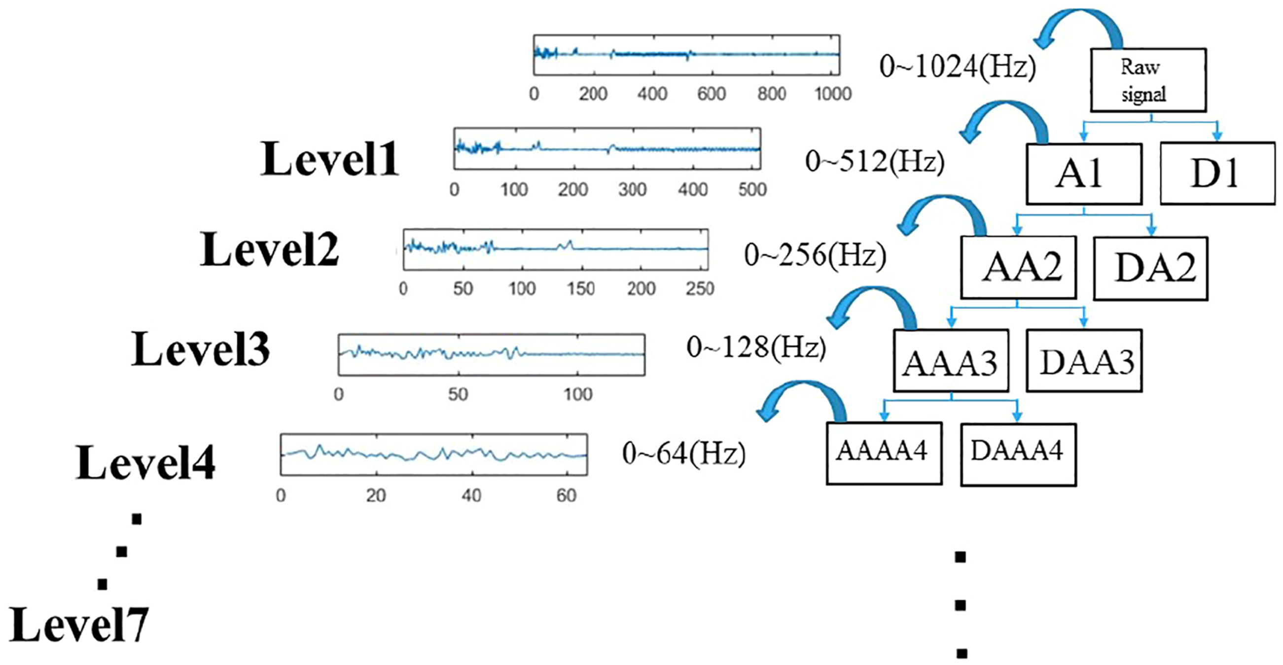

Experimental results and discussion

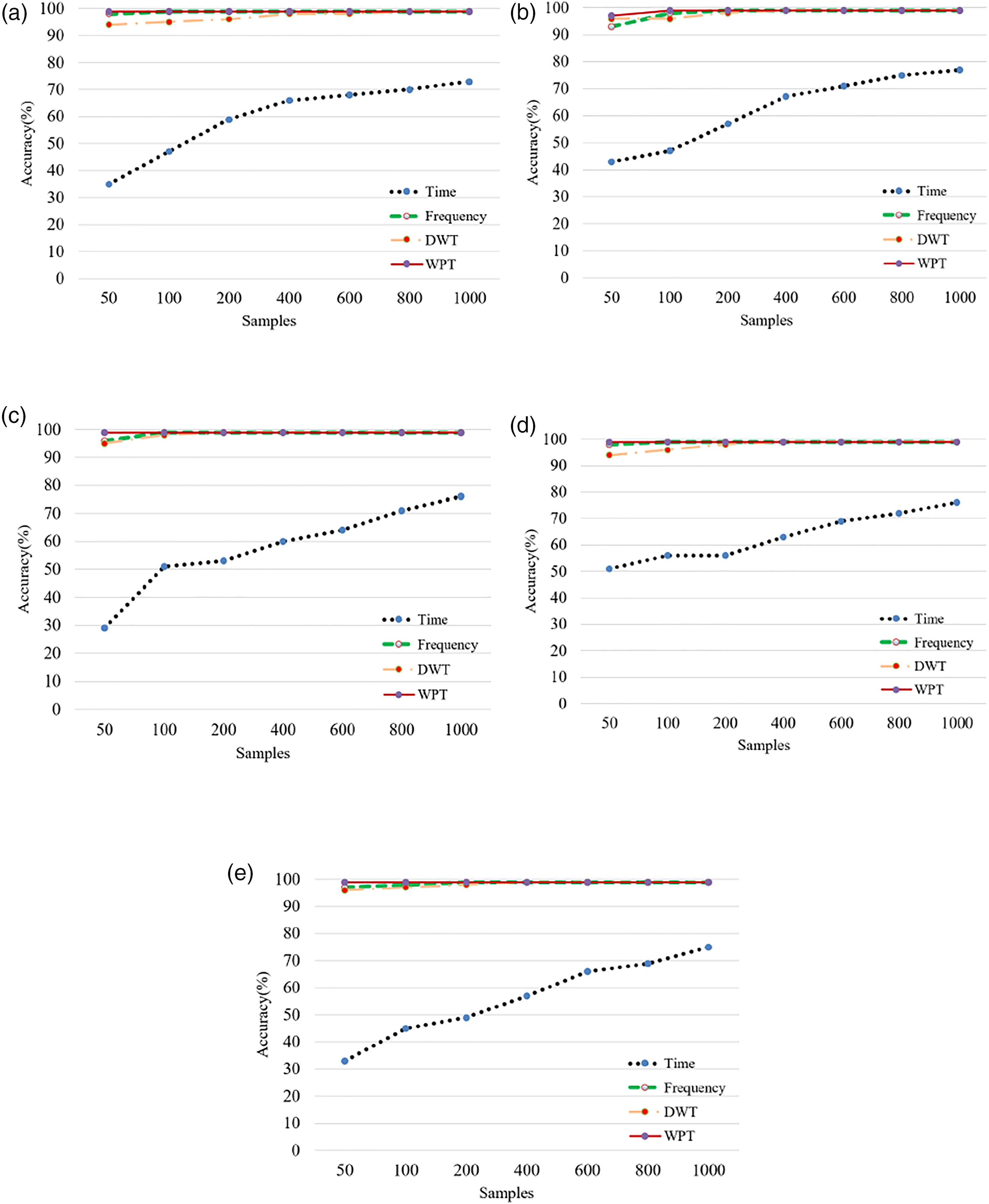
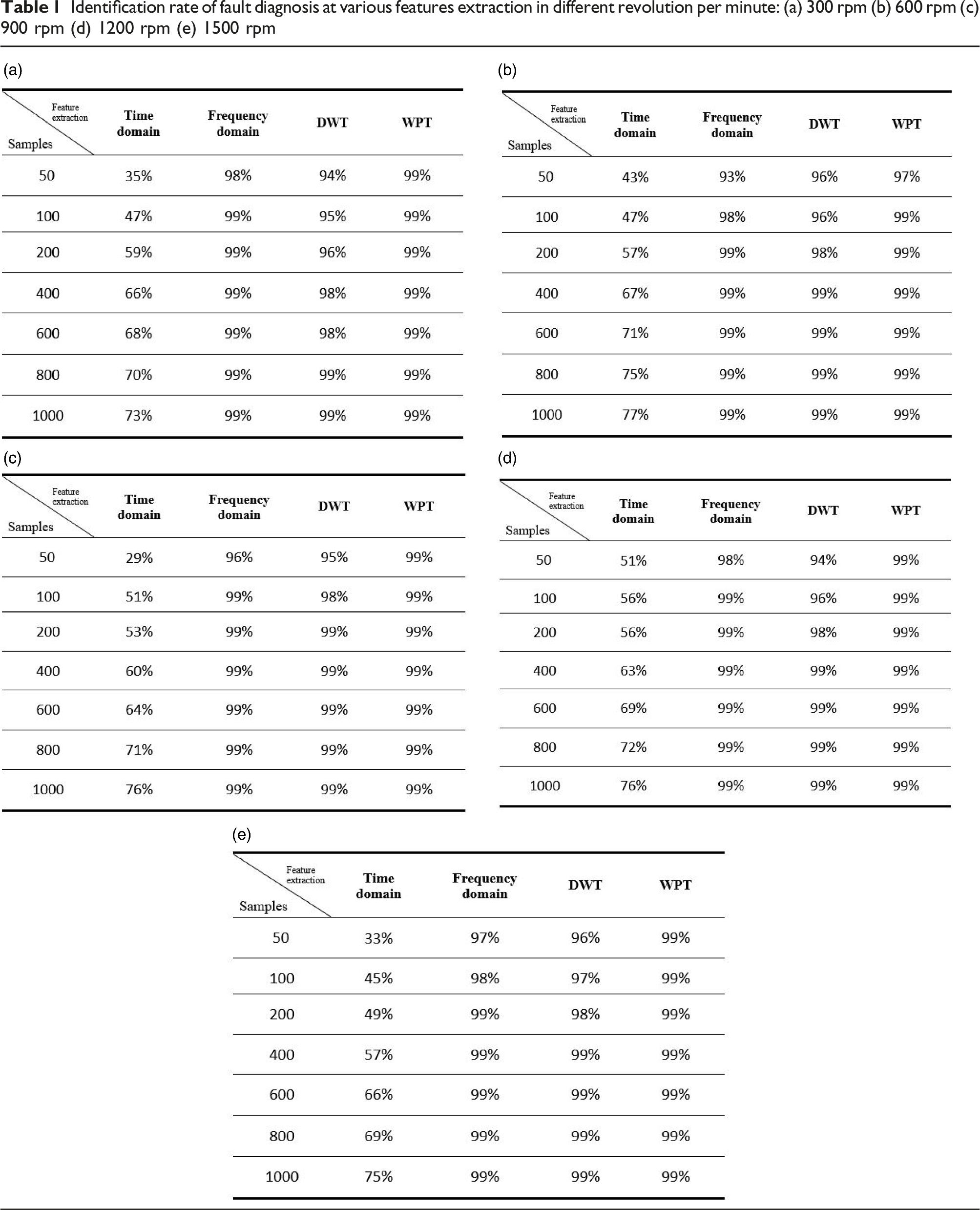
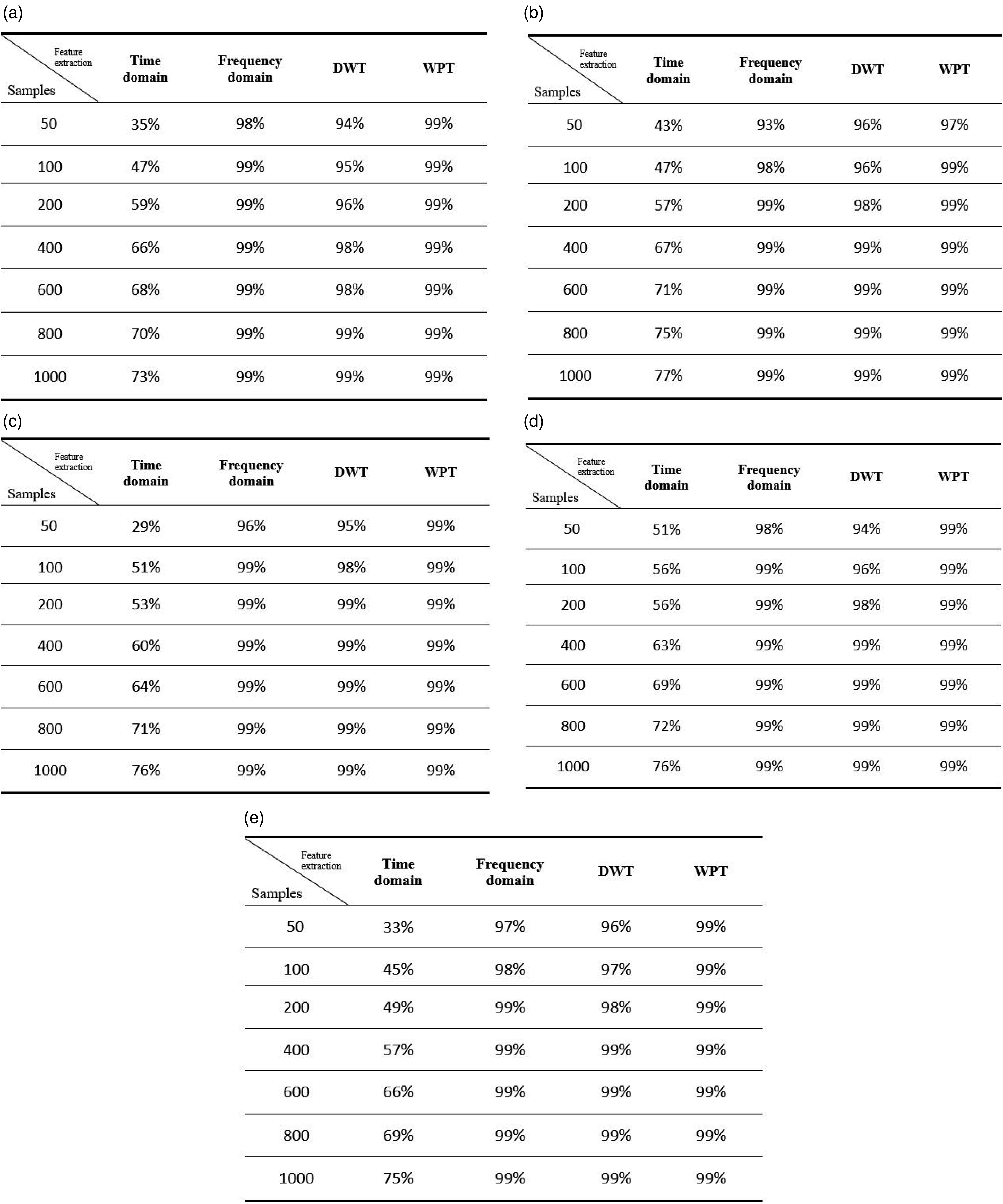
The signal is used to enter three different feature extraction methods, and the four-signal data serves separately as an input into the deep neural network for classifying the fault diagnosis. The flow chart of signal classification is shown in Figure 18. The experimental result recognition rate is summarized in Figure 19, the relationship between the number of samples of the four signals at five speeds and the recognition rate of classification fault diagnosis can be seen from the curve. Regardless of which speed, the recognition rate in the time domain is the lowest. Because it only reached 70% when 1000 samples were trained. After three feature extractions such as FFT, DWT, and WPT, when the number of samples is 50, the recognition rate can reach more than 90%, each speed recognition rate is not the same. When the sample number is trained to 400, the FFT, DWT, and WPT recognition rates can reach 99%. The WPT recognition rate is the best. In the case of 50 samples, no matter which speed is higher than the other three signals, the recognition rate is high in the case of sample 100, WPT can achieve 99% recognition rate per revolution. Table 1 summarized the identification rates of proposed experiment in fan revolution 300 to 1500 rpm.

Figure 18.

Flow chart of signal classification.

Figure 19.

Identification rate of fault diagnosis at various features extraction in different revolution per minute: (a) 300 rpm (b) 600 rpm (c) 900 rpm (d) 1200 rpm (e) 1500 rpm

Table 1

Identification rate of fault diagnosis at various features extraction in different revolution per minute: (a) 300 rpm (b) 600 rpm (c) 900 rpm (d) 1200 rpm (e) 1500 rpm

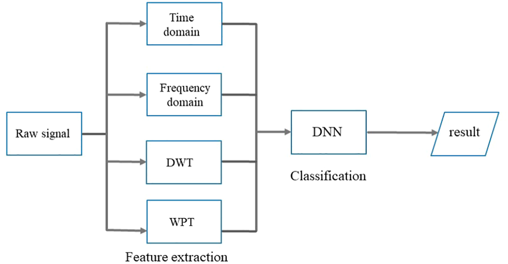
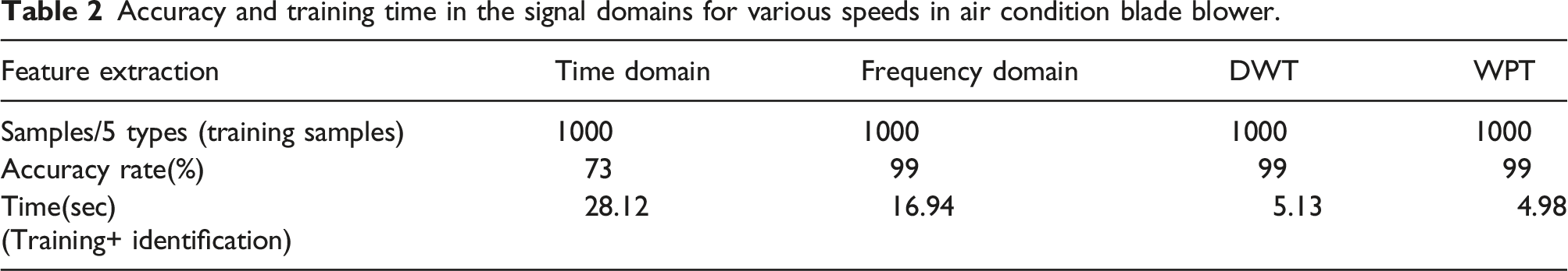
Table 2 summarized the recognition rate and recognition time of the four signals under the same training sample. It can be seen from the results that the recognition rate in the time domain through deep learning classification is the lowest and the training time is the longest. In terms of analysis, the system’s discrimination has improved. The experimental results also reflect the recognition rate, which can reach 99%, but the recognition time cannot be reduced a lot, but after DWT, the energy characteristic value decomposed from the low-frequency middle layer of the signal. Not only the recognition rate can also be up to 99%, the recognition time is much shorter than the time and frequency domains. Finally, the eigenvalues of low-frequency and high-frequency signals are decomposed by WPT. This not only makes the characteristic value of the entire signal more comprehensive, but also makes the recognition rate higher. It has 99% performance and is shorter than DWT in training recognition time. Experimental results show that WPT is superior to the other three signal feature extraction.

Table 2

Accuracy and training time in the signal domains for various speeds in air condition blade blower.

Feature extraction	Time domain	Frequency domain	DWT	WPT
Samples/5 types (training samples)	1000	1000	1000	1000
Accuracy rate(%)	73	99	99	99
Time(sec) (Training+ identification)	28.12	16.94	5.13	4.98

Conclusions

This study matches five different speeds and five different conditions of the blower, and then the four different feature extraction methods of time domain, frequency domain, DWT and WPT are used to establish the data volume of different feature extraction. Through deep learning, the vehicle air-conditioning blower fault diagnosis is performed. The experimental results show that the frequency domain recognition rate and training plus recognition time are far away. It is higher than the time domain, but because DWT can decompose the low-frequency middle layer of the sound signal and extract the energy characteristic value, not only does the recognition rate perform very well like the frequency domain, it is far more than the previous two in training plus recognition time It is much shorter, the principle of WPT is the same as that of the DWT system. It can not only decompose low-frequency signals, but also high-frequency signals. In terms of training and recognition time, it can be shorter than DWT. WPT combined with deep learning can make this car blower fault diagnosis system achieve better performance.

Footnotes

Declaration of conflicting interests

The author(s) declared no potential conflicts of interest with respect to the research, authorship, and/or publication of this article.

Funding

The author(s) disclosed receipt of the following financial support for the research, authorship, and/or publication of this article: The study was supported by the Ministry of Science and Technology of Taiwan, Republic of China, under project number MOST 109-2221-E-018-013.

ORCID iD

Jian-Da Wu

References

Gencoglu

Virtanen

Huttunen

Recognition of acoustic events using deep neural networks. The 22nd European Signal Processing Conference (EUSIPCO), Lisbon, Portugal, 1–5 Sept 2014. 2014. 506–510.

Kim

Chae

, et al. Deep neural network-based automatic modulation classification technique. International Conference on Information and Communication Technology Convergence (ICTC), Jeju Island, South Korea, 20–22 Oct 2021. 2016. 579–582.

Huang

, et al. The development of a deep neural network and its application to evaluating the interior sound quality of pure electric vehicles. Mech Syst Signal Process 2019; 120: 98–116.

Huang

, et al. Novel method for identifying and diagnosing electric vehicle shock absorber squeak noise based on a DNN. Mech Syst Signal Process 2019; 124: 439–458.

Benko

Petrovcic

Juričić

, et al. An approach to fault diagnosis of vacuum cleaner motors based on sound analysis. Mech Syst Signal Process 2005; 19(2): 427–445.

Mallat

. A theory for multiresolution signal decomposition: the wavelet representation. IEEE Trans Pattern Anal Mach Intell 1989; 11(7): 674–693.

Mallat

. Multifrequency channel decompositions of images and wavelet models. IEEE Trans Acoust 1989; 37(12): 2091–2110.

Mallat

. Multiresolution approximations and wavelet orthonormal bases of L 2 (R). Trans Am Mathematical Society 1989; 315(1): 69–88.

Ehya

Nysveen

Skreien

. Performance evaluation of signal processing tools used for fault detection of hydrogenerators operating in noisy environments. IEEE Trans Ind Appl 2021; 57(4): 3654–3665.

10.

Mathew

Zhang

. Acoustic-Based Engine Fault Diagnosis Using WPT, PCA and Bayesian Optimization. Appl Sci 2020; 10(19): 6890.

11.

Djurovi

. Estimation of the sinusoidal signal frequency based on the marginal median DFT. IEEE Trans Signal Process 2007; 55(5): 2043–2051.

12.

Liu

, et al. Automatic modulation recognition of digital signals using cwt based on optimal scales. The 2014 IEEE International Conference on Computer and Information Technology, Xi’an, China, 11–13 September 2014. 2014. 430–434.

13.

Shirazi

Mahjoob

Application of discrete wavelet transform (DWT) in combustion failure detection of IC engines. The 2007 5th International Symposium on Image and Signal Processing and Analysis, Istanbul, Turkey, 27–29 Sept 2007. 2007. 482–486.

14.

Chen

Zhang

Yang

, et al. Research for adaptive audio information hiding approach based on DWT. The 2008 Chinese Control and Decision Conference, Yantai, China, 2–4 July 2008. 2008. 3029–3033.

15.

Haripriya

Mathew

Gopakumar

Performance evaluation of dwt based speech enhancement. The 2017 International Conference on Networks & Advances in Computational Technologies (NetACT), Thiruvananthapuram, India, 20–22 July 2017, 2017. 442–446.

16.

Wang

Han

Wang

, et al. Speech recognition based on wavelet packet transform and KL expansion. The 2008 Chinese Control and Decision Conference, Yantai, China, 2–4 July 2008. 2008. 2490–2493.

17.

Wan

The fault diagnosis method of rolling bearing based on wavelet packet transform and zooming envelope analysis. The 2007 International Conference on Wavelet Analysis and Pattern Recognition, Beijing, China, 2–4 Nov 2007. 2007. 1257–1261.

18.

Kim

Chun

Cho

Evaluation of noise reduction in experimental battery pack voltage using discrete wavelet transform and wavelet packet transform. The 2015 IEEE International Telecommunications Energy Conference (INTELEC), Osaka, Japan, 18–22 Oct 2015. 2015. 1–5.

19.

Karmakar

Kumar

Patney

. Design of optimal wavelet packet trees based on auditory perception criterion. IEEE Signal Process Lett 2007; 14(4): 240–243.

20.

Manusov

Makarov

Dmitriev

, et al. Training sample dimensions impact on artificial neural network optimal structure. The 2013 12th International Conference on Environment and Electrical Engineering, Wroclaw, Poland, 5–8 May 2013. 2013. 156–159.

21.

Harun

Dlay

Woo

Performance of keystroke biometrics authentication system using Multilayer Perceptron neural network (MLP NN). The 2010 7th International Symposium on Communication Systems, Networks & Digital Signal Processing (CSNDSP 2010), Newcastle Upon Tyne, UK, 21–23 July 2010. 2010. 711–714.

22.

Y-j

, et al. Tooth decay diagnosis using back propagation neural network. The 2006 International Conference on Machine Learning and Cybernetics, Dalian, China, 13-16 Aug 2006. 2006. 3956–3959.

23.

Endah

Widodo

Fariq

, et al. Beyond back-propagation learning for diabetic detection: convergence comparison of gradient descent, momentum and Adaptive Learning Rate. The 2017 1st International Conference on Informatics and Computational Sciences (ICICoS), Semarang, Indonesia, 15–16 Nov. 2017. 2017. 189–194.

24.

Kim

, et al. Performance of deep learning computation with TensorFlow software library in GPU-capable multi-core computing platforms. The 2017 Ninth International Conference on Ubiquitous and Future Networks (ICUFN), Milan, Italy, 4–7 July 2017. 2017. 240–242.

25.

Schwiebert

Boosting Python performance on Intel Processors: A case study of optimizing music recognition. The 2016 6th Workshop on Python for High-Performance and Scientific Computing (PyHPC), Salt Lake City, Utah, 13–18 November 2016. 2016. 52–58.

26.

Massiris

Dennehy

Delrieux

, et al. Python implementation of local intervoxel-texture operators in neuroimaging using Anaconda and 3D Slicer environments. The 2017 XLIII Latin American Computer Conference (CLEI), Córdoba, Argentina, 4–8 September 2017. 2017. 1–3.

Fault diagnosis for vehicle air conditioning blower using deep learning neural network

Abstract

Keywords

Introduction

Principle of noise feature extraction and deep neural network

Discrete wavelet transform

Wavelet packet decomposition

Structure of deep learning neural network

Learning framework

Python language

Implementation and experimental work of blower fault diagnosis

Experimental work and data measurement

Blade blower sound signal processing

Experimental results and discussion

Conclusions

Footnotes

Declaration of conflicting interests

Funding

ORCID iD

References