Predicting the dynamic response of a structure using an artificial neural network

Abstract

Machine learning and artificial intelligence has been applied to other facets of structural mechanics and structural dynamics, mainly for structural optimization and structural reliability analysis, but have seen little use in surrogate modeling for structural time series prediction. The current research will focus on how data reduction tools (such as mathematical morphology) can be applied to dynamic structural data and can be used in conjunction with clustering methodologies as well as artificial neural networks (ANNs) to create a useful and highly computationally efficient dynamic model that can be used to make predictions on the acceleration response of a structural system. The current study utilizes training data developed from finite element modeling of a simple system that demonstrates a nonlinear behavior of interest (a change in the dynamic response with a change in loading magnitude), but the methodologies developed could be applied to other modeling or analysis schemes, test data, or in-situ measurements of a structure of interest. The results of the study show how mathematical morphology tools can reduce the dimensionality of time series data while still preserving important characteristics like natural frequency, and the use of ANNs shows promise as a surrogate model for dynamic response prediction.

Introduction

Large companies like Facebook and Google have benefitted widely from the application of machine learning and artificial intelligence (AI) techniques on the vast amount of data that they use and generate. ¹ In the field of structural mechanics, machine learning has been applied in areas such as but not limited to structural optimization, structural health monitoring (SHM), and structural reliability analysis. Specifically in the area of structural dynamics, work has been conducted on surrogate models that predict dynamic characteristics of structures, such as natural frequency, but little attention has been given to areas where time series data prediction is of interest due to the higher dimensionality of outputs. ² In Noël and Kerschen, ² a systematic and cohesive review of progress in this field is provided, defining the most prominent progress addressing complex nonlinearities in larger scale structures. The field of structural mechanics and dynamics also often deal with large amounts of data and have benefited from the exploration and application of machine learning and AI. ³

Previous uses for machine learning and AI in the field of structural mechanics falls into three main areas of interest: structural optimization, structural reliability analysis, and SHM. The first area of interest is design optimization using heuristic algorithms. These heuristic algorithms can sample the data and home in on multiple optimums at once, making them extremely robust and computationally efficient. Kicinger et al. ⁴ present a comprehensive review of the use of a type of heuristic algorithm known as evolutionary algorithms (EAs). These EAs rely on “populations” of “individuals” that are represented by a set of “genes” and have a particular “fitness.” This model can be used in structural design to optimize the topology (layout), shape, and sizing of members in structures to minimize weight, stress, and deflection all at the same time. ⁴ The particle swarm optimization (PSO) method uses a slightly different but still very practical approach to structural optimization based on the social interactions between birds, fish, bees, and other animals that flock to seek food sources and avoid predators. ⁵ PSO is utilized to minimize the weight of 10 bar, 25 bar, and 72 bar truss structures while maintaining strength and stiffness criteria. ⁵ Many more of these algorithms exist and have been applied to structures of interest (teaching–learning based optimization, ⁶ elitist self-adaptive step-size search, ⁷ and ant colony optimization ⁸ ), all of which attempt to use AI and heuristic algorithms to optimize structures with varying levels of success.

Structural reliability analysis is another area of structural mechanics that benefit from the use of machine learning and AI. Artificial neural networks (ANNs) are one main form of machine learning currently being used in the field of structural analysis. ANNs are computing systems loosely based on the structure of the human brain, consisting of one or multiple layers of “neurons” connected by “synapses” that can transmit signals and be trained to deliver a set of outputs given a certain set of input parameters. ⁹ Chojacyk et al. ⁹ present a review of the application of ANNs to the structural reliability and optimization of steel structures. The long-standing standard for structural reliability analysis has been the Monte Carlo simulation (MCS) method, which performs limit state evaluations to be able to approximate the probability of structural failure. ⁹ The main issue with this method is the computationally expensive task of generating the limit state function which can often have an implicit form. ⁹ The study concludes by applying the ANN and MCS combination to a stiffened steel plate, comparing results to ones found using a nonlinear finite element analysis. ⁹ Cardoso et al. ¹⁰ used similar methodology to optimize a steel structure using the structural reliability analysis as a design constraint. In this case, an ANN was used as a proxy model and a genetic algorithm was utilized for optimization. The methodology was applied to a simple steel frame and a six-bar truss to optimize them based on the lowest probability of failure. This resulted in a model consistent with the utilization of an MCS but required significantly less computational resources. ¹⁰

Structural health monitoring is the third and final area of interest and refers to the process of detecting damage for aerospace, civil, or mechanical structures while the structure of interest is in use. The process involves monitoring the dynamic or other measured response and extracting damage-sensitive features from these measurements. A statistical analysis is then performed to determine the current state of health of the system. ¹¹ In Worden and Manson, ¹² drilled holes and saw cuts were applied to a panel in a controlled way, representative of damage on an airplane wing. To determine if damage was present, the authors assessed the transmissibility (or ratio of acceleration spectra) between two points when the panels were subjected to excitations. A characteristic plot for the transmissibility was determined for undamaged panels and panels that were damaged in various ways. An outlier analysis was performed to characterize each dataset. A Monte Carlo method was utilized to determine a threshold, where any dataset in the outlier analysis that fell below the threshold was indicative of undamaged patterns. In a related study, a network of sensors were attached to the wing of an aircraft (which the previous panels were representative of), and inspection panels at various locations on the wing were removed to simulate damage without inflicting actual damage. ¹² A multi-layer perceptron neural network was trained using transmissibility data of the structure in various damaged states (various panels removed or installed) to be able to predict the state and location of damage. The model was able to classify various “damaged” states to within 85.6% accuracy, with most of the classification error due to particular panel sets. ¹²

In addition to these areas of engineering, in the world of structural dynamics, surrogate models have become increasingly popular for predicting the dynamic behavior of structures of interest. Specifically, Le and Caracoglia used an ANN trained on numerically generated responses of a vertical structure subjected to tornadic wind loads. ¹³ The resulting ANN could be used to aid in life-cycle cost assessment in an economical and efficient manner. ¹³ In a similar study, a finite element model of a bridge was used in additional to actual measured data to train an ANN on the buffeting responses of a bridge subjected to a variety of wind loads. ¹⁴ Both of these studies utilize machine learning models as surrogate models for structural dynamic data prediction, but neither attempt to predict time series response directly. The main issue in this area is the high dimensionality of dynamic data, which can make many traditional data analysis techniques intractable. ¹⁵

As technology progresses and its complexity increases so does the complexity of the data that is generated. Whereas before large quantities of data were collected and assumed to consist of a few variables, today data are collected with such fine detail that datasets can consist of hundreds of unique variables, rendering many traditional data analysis techniques useless. ¹⁵ Single data observations now can be entire curves or spectra (images for example), which makes it difficult for rapid analysis. ¹⁵ Although statistical models do exist, training these models becomes intractable when applied to higher dimension data. ¹⁵ Models like linear regression can still be applied to moderate dimension data models, given that some linearity still exists, but once dimensions get too high, applying methods like linear regression becomes much too computationally expensive. ¹⁶ Data collection today is not as methodical as it once was, mostly because researchers and scientists are not entirely sure what variable they are interested in. ¹⁵ This results in the massive collection of complex data and no real way to sift through it. Donoho compares it to “finding a needle in a haystack.” ¹⁵ This problem looms large, and there are already many fields dedicated to dealing with high dimensional data.

Structural dynamics deals with a major form of high dimensional data: time series data. Data in this form can cause difficulties with analyzing the behavior of dynamic systems because strategies like clustering are not always able to deal with the added dimensionality. ¹⁷ Dynamic datapoints are not standalone, they depend on the datapoint preceding and following itself, which slows down many clustering techniques. ¹⁷ There are machine learning tools to tackle problems with data in this form, such as recurrent neural networks, but the lack of interpretability and increased complexity that comes along with these models was seen as a worse trade-off when compared to the tools used in this study. ¹⁸

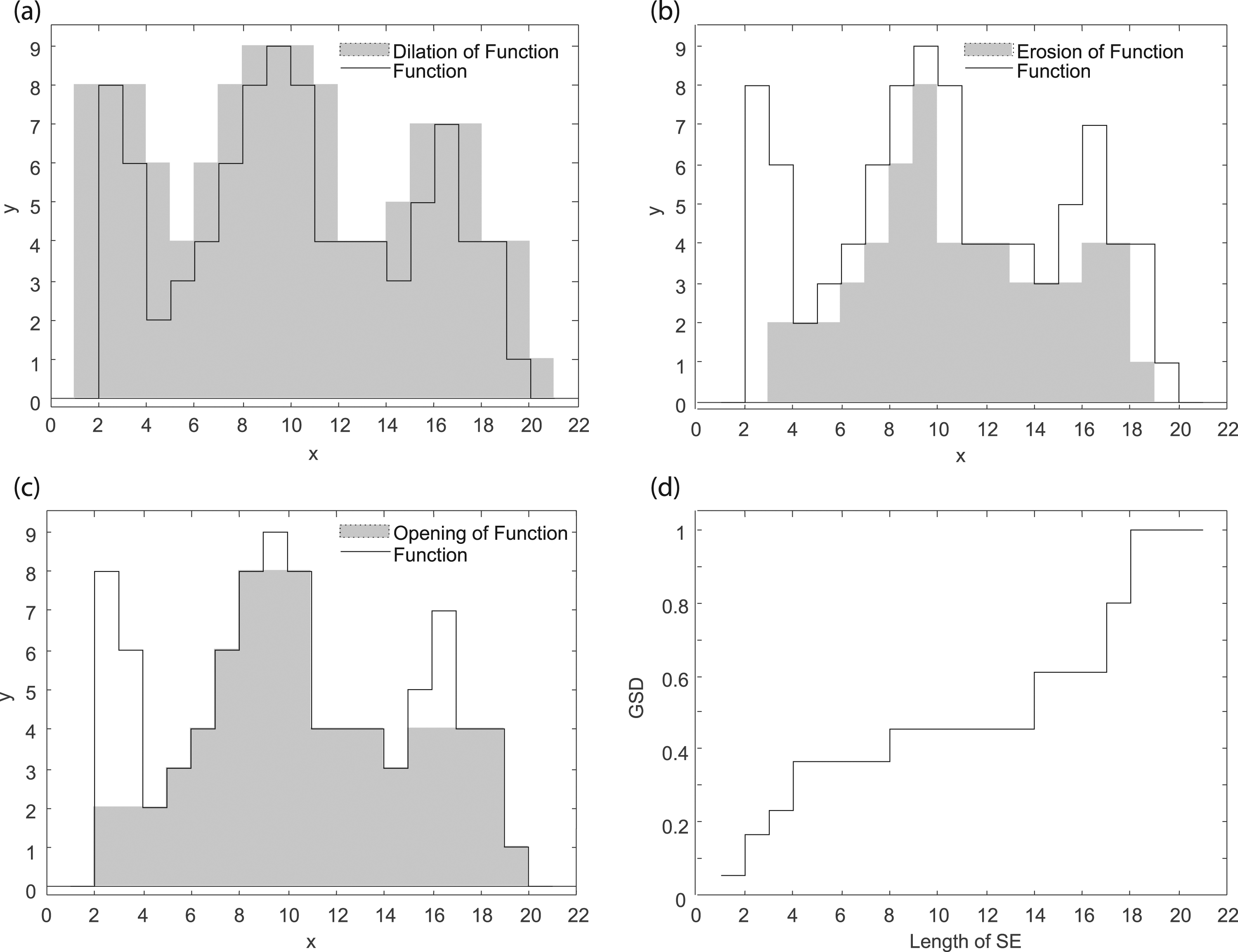
One useful tool that can be used to decrease the dimensionality of data is mathematical morphology (MM). MM tools are utilized to study the geometric structures of images, graphs, or other topologies. MM operators work by probing shapes with smaller shapes known as structuring elements (SE) to extract relevant information about the shape. ¹⁹ Using MM operations, the Granulometric Size Distribution (GSD) can be defined. ²⁰ An analogy can be made to geotechnical engineering, where a GSD of a soil sample is created by sifting the sample through a series of sieves with varying mesh sizes. ¹⁹ The amount of soil that is retained by each sieve is recorded, which then generates the GSD curve for the sample. ¹⁹ This same type of process can be applied to data using MM operators. Using MM operators like opening, the amount of data cut off by the operation can be recorded for each SE size used, then graphed to form a GSD of the data. This resulting curve represents a higher dimensionality curve with significantly less dimensionality, while still preserving the general shape of the original data. ¹⁹

Data reduction techniques like the GSD have already been applied to other areas of engineering, specifically dealing with solar irradiation curves ¹⁹ and electromagnetic emissions. ²⁰ Gastòn-Romeo et al. ²⁰ describe and utilize the methodology of the GSD to convert daily solar radiation curves into GSDs. This, in turn, reduces their dimensionality and allows various clustering methodologies to be applied to group the data into sunny days, rainy days, etc. ²⁰ The methodology would be extremely useful for thermal plants looking to scout an area for its viability (more sunny days is desirable). ²⁰ Similarly, the GSD has been applied to solar irradiation curves to eliminate noise and detect unusual solar emissions. ¹⁹

These data reduction tools can be utilized to make clustering techniques more usable and efficient . ¹⁷ A vast number of these clustering methodologies exist. Rousseeuw and Kaufmann provide a fundamental overview of many of the most common methodologies. ²¹ The PAM algorithm (partitioning around medoids), for example, PAM clusters data by selecting a specified number of datapoints as medoids and proceeds to minimize the distance between that medoid and other datapoints that are specified to be in that cluster. ²¹ Another popular clustering methodology is known as hierarchical clustering. This methodology can use any clustering method, but this time applies the clustering multiple times, creating multiple layers of data clusters. ²² This method can be useful for diving deeper into clusters that may not appear just from methods like PAM but fails in cases where the initial clustering layer is not ideal. ²¹ These clustering methodologies can all be used to find underlying structures in data. Within structural dynamic data, methodologies like these can help reveal hidden information about the system in question. ²¹

Machine learning and AI has been applied to other facets of structural mechanics and structural dynamics, mainly for structural optimization and structural reliability analysis, ⁹ but these techniques have seen little use in the direct prediction of time series data for a structure of interest. This study will be focused on filling this gap to try and create more computationally efficient solutions for modeling the dynamic behavior of structures. The current research will focus on how data reduction tools (such as MM) can be applied to dynamic structural data and can be used in conjunction with clustering methodologies as well as (ANNs) to create a useful and highly computationally efficient dynamic model that can be used to make predictions on the acceleration response of a structural system. If effective, these tools could save significant computational and testing resources in civil and structural fields of engineering.

Methodology

The goal for this research was to make predictions about the dynamic response of a nonlinear structural system using machine learning, rather than more computationally expensive, physics-based finite element models. The purpose of this is to explore the potential of machine learning tools for making dynamic predictions, as it would save computational and testing resources when gathering data on a structure of interest. To do this, the acceleration response taken from a nonlinear dynamic model will be utilized and converted into GSD curves. For the current study, a simplified finite element model is utilized to generate the dynamic response, but the methodology could be applied to dynamic test data of a structural system or data from a structure that is currently in use. Clustering methodologies are applied to the GSD curves to identify groups or clusters with similar responses. A portion of generated GSD curves were removed and the rest utilized to train an ANN to take the input parameters of the model and produce GSD curves. The predicted curves were then re-clustered so that a characteristic acceleration curve could be selected from the appropriate cluster, completing the ANNs ability to go from input parameters to output acceleration time history. This effectively compares the ability of the ANN technique proposed here to the traditional approach for modeling the dynamic response of civil structures: the finite element method.

The cantilever beam model

A simplified structural model was developed using the finite element software ABAQUS for this research with the goal of having a tool to produce an acceleration response that was nonlinear with input loading. Although a model was used to generate data for the current study, experimental data or data from a structural system in-use could just as easily be applied. The ideal structural model for this analysis was one that yielded a nonlinear response to loading, but that was also as simple as possible. This resulted in the creation of a cantilever beam model that is fixed on one end (nodes fully constrained), while the other end is left free. The beam is subjected to a positive thermal load, which strains the free end of the beam into a fixed wall with friction. The member is then subjected to a pressure impulse loading on the top side of the beam. The input parameters to the model include the coefficient of expansion ( $\alpha$ ) for the beam material, the coefficient of friction ( $\mu )$ between the beam end and the wall, the applied pressure load (P), and the width (w) and thickness (t) of the beam. The resulting cantilever beam model is shown in Figure 1, and the values used for the parameters shown are defined in Table 1.

Figure 1.

(a) Schematic of beam model. (b) The 3-dimensional finite element mesh of the beam. (c) First bending mode of the beam in the fixed-fixed response. (d) End response of beam pressed against wall.

Table 1.

Nominal configuration for the cantilever beam model (highlighted parameters were not varied).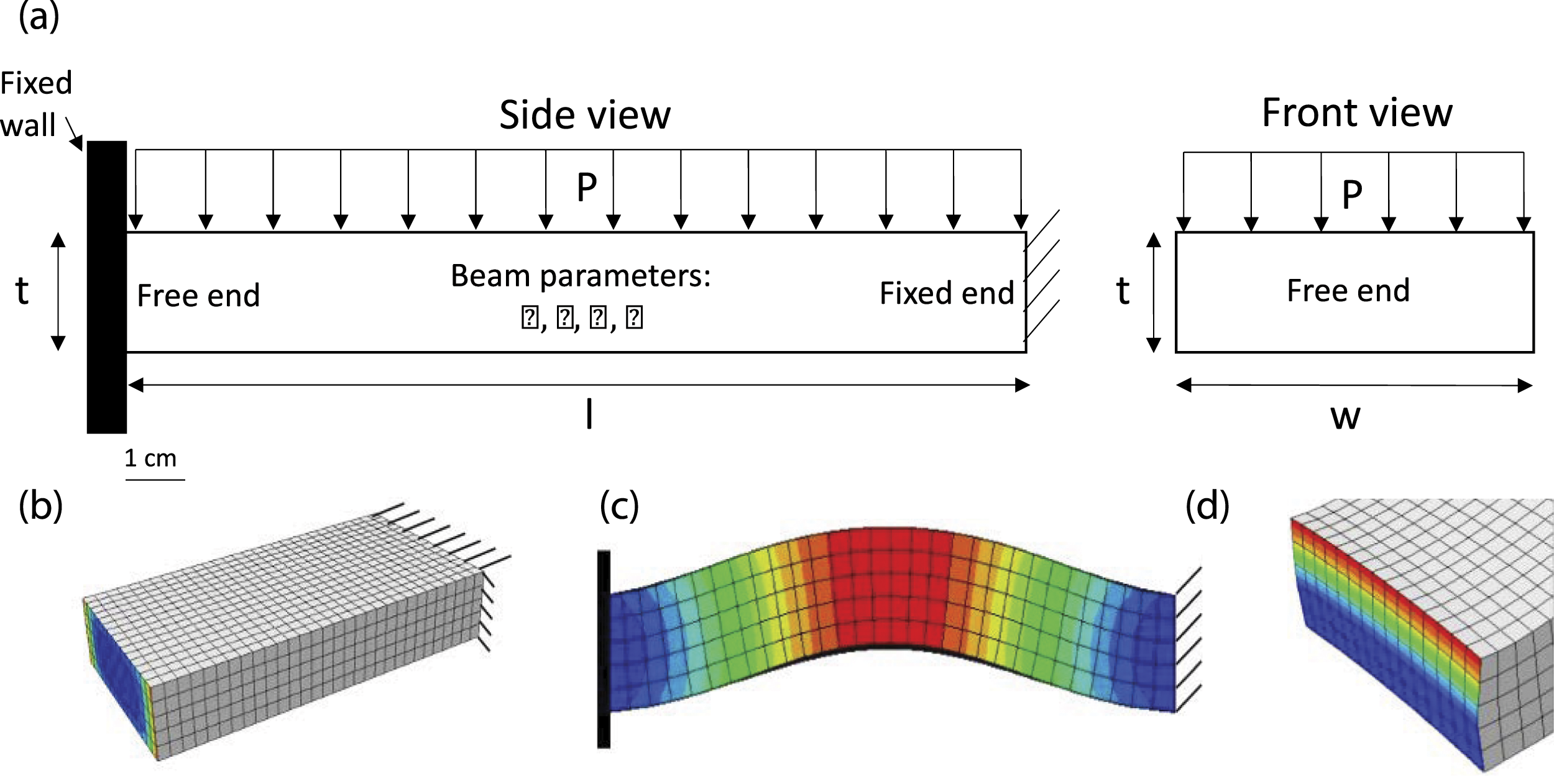

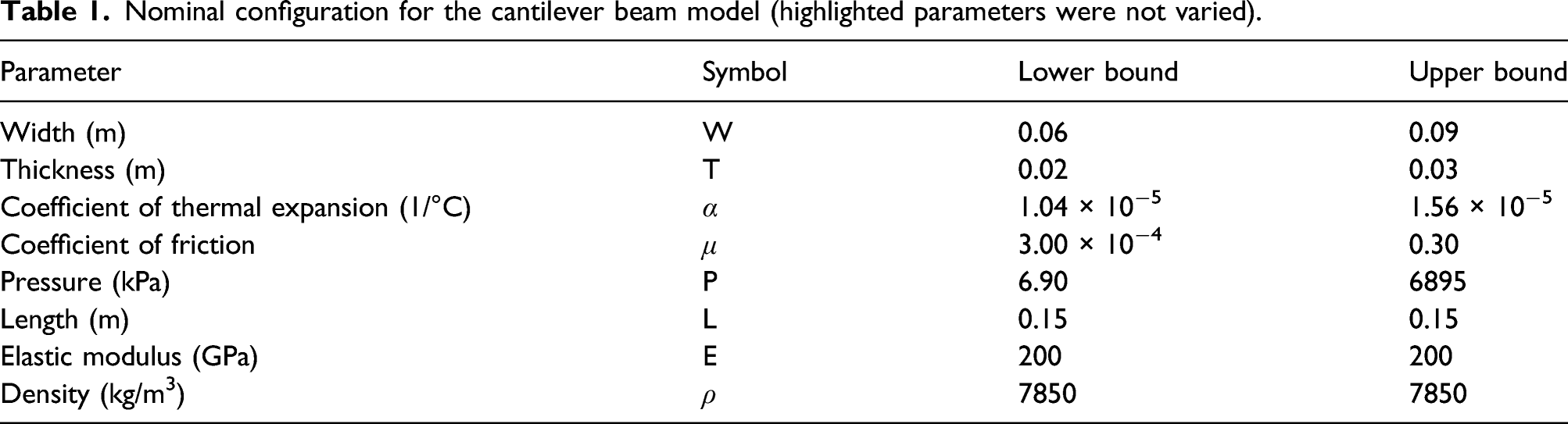
Parameter	Symbol	Lower bound	Upper bound
Width (m)	W	0.06	0.09
Thickness (m)	T	0.02	0.03
Coefficient of thermal expansion (1/°C)	$\alpha$	1.04 × 10−5	1.56 × 10−5
Coefficient of friction	$\mu$	3.00 × 10−4	0.30
Pressure (kPa)	P	6.90	6895
Length (m)	L	0.15	0.15
Elastic modulus (GPa)	E	200	200
Density (kg/m3)	$\rho$	7850	7850

The constitutive model used to describe the beam’s material is a simple linear elastic material with a Young’s modulus similar to steel. The entire response of the beam is assumed to behave linear elastically. The nonlinear behavior described is due to the friction interaction between the end of the beam and the fixed wall. Considering two loading scenarios, one with low pressure loading and high coefficient of friction, the other with high pressure loading and low coefficient of friction, the nonlinearity can be observed. In the first case, the response would be similar to a fixed–fixed beam’s response, while the other would be more like a fixed-free response. Therefore, with different loading scenarios, the response can produce completely different modes. This represents the desired nonlinearity for this model. This nonlinear behavior is demonstrated in Figure 2 for two test cases where acceleration was determined at the mid-span of the beam.

Figure 2.

The nonlinear response of two different configurations of the cantilever beam, including top: applied pressure, middle: acceleration response, and bottom: frequency response.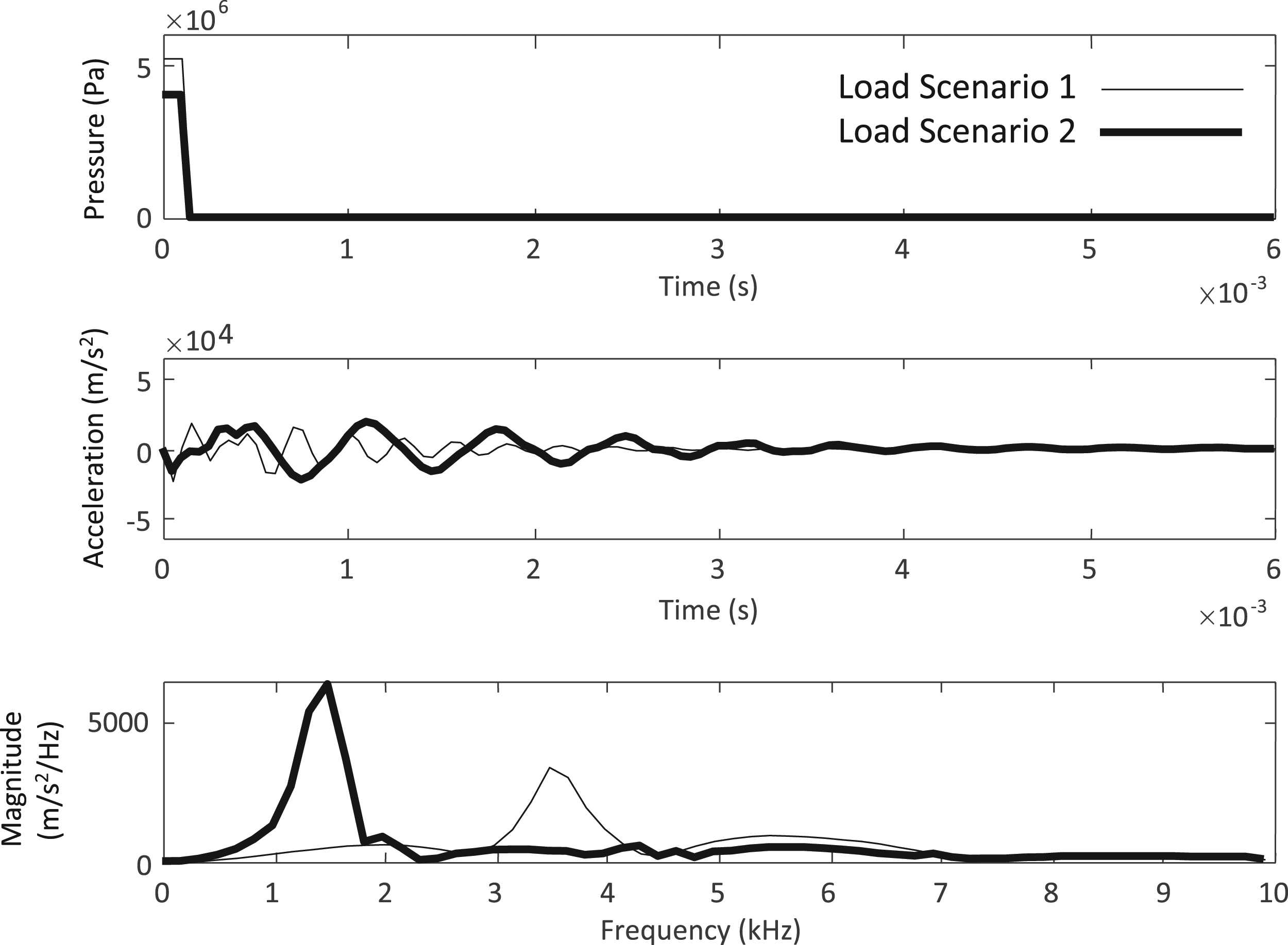

Figure 2 shows that even with slight variation in pressure loading, the beam model’s frequency response can change drastically. This demonstrates the nonlinear behavior that was desired. The model included parameterization for block thickness, width, length, modulus of elasticity, coefficient of thermal expansion, coefficient of friction, and the magnitude of the pressure load. The nominal configuration for the cantilever beam is shown in Table 1.

The parameters were randomly sampled between the lower and upper bounds shown in Table 1, except the length of the beam, elastic modulus, and density (highlighted) which were all kept constant. The pressure loading and coefficient of friction had a larger range to center the domain on the output of interest. In the end, a total of 200 analyses were conducted. The output parameter of interest was the acceleration time history of both the end and mid-span of the beam. Either of these parameters could be used without affecting the methodology used in this study.

Creation of the granulometric size distribution

The method for creation of the GSDs comes primarily from Guardiola et al. ¹⁹ and Gastón-Romeo et al. ²⁰ This method relies on the use of MM, which is defined as the theory and techniques for the analysis of spatial structures such as the shape and size of objects. ¹⁹ The goal with using these data reduction tools is so that the acceleration time series data, which is many datapoints where every point depends on the point before and after it, can be converted into a much smaller dataset that can uniquely describe each acceleration curve. The mathematic operators that will be used in this study are erosion, dilation, and opening.

To understand these operators, an arbitrary function $f\left(x\right)$ will be considered. MM operators work by probing shapes with smaller shapes known as a structuring element. An SE can be one, two or three dimensions and take on multiple shapes. When probing a function, a line segment will be utilized as the SE. This line segment will be called $B$ and will extend from point a to point b, denoted as $\left(a,b\right)$ . The length of this SE will then be defined as $\lambda$ , where $\lambda =b-a$ . The first operation that will be defined is a dilation, which intuitively can be seen as expanding a shape by the size of the SE. The dilation, ${\delta }_B$ , of a function $f\left(x\right)$ using SE $B$ can be defined using equation (1) ¹⁹

$${\delta }_B\left(f\left(x\right)\right)=ma{x}_{b\in B}f\left(x+b\right)$$

(1)

An erosion essentially does the opposite of a dilation, shrinking an image by the size of the structuring element. The erosion, ${\in }_B$ , of a function $f\left(x\right)$ using SE $B$ can be defined using equation (2) ¹⁹

$${\in }_B\left(f\left(x\right)\right)=mi{n}_{b\in B}f\left(x+b\right)$$

(2)

Finally, the opening function can be defined, which consists of an erosion followed by a dilation, and is seen intuitively as cutting the tops off the curve. The opening, $o_B$ , of a function $f\left(x\right)$ using SE $B$ can be defined using equation (3) ¹⁹

$$o_B\left(f\left(x\right)\right)={\delta }_B\left({\in }_B\left(f\left(x\right)\right)\right)$$

(3)

Using these operators, the GSD can be defined. Traditionally used in areas of civil engineering, the GSD is a way of representing the various sizes of aggregate found in samples of soil. A soil sample is run through a number of different sieves, starting with the smallest size and gradually increasing, recording the amount remaining in each sieve. The GSD represents the amount of soil left on each sieve size. Similarly, using the opening operation on a graphed curve, the amount of data removed using each SE size can be recorded and used to create a representative GSD curve of the data. The GSD of function $f\left(x\right)$ is defined in equation (4) ¹⁹

$$\mathrm{GSD}\left(f\left(x\right)\right)=1-\frac{m\left(\lambda \right)}{m\left(0\right)}$$

(4)

Where $m\left(\lambda \right)$ is the area under the opening curve for each SE of length $\lambda$ . Figure 3 shows the three MM operators being applied to an arbitrary step function using a structuring element of length 2, along with the GSD curve resulting from repeated opening operations on the function.

Figure 3.

The (a) dilation, (b) erosion, and (c) opening of an arbitrary step function and the corresponding granulometric size distribution (GSD) shown in (d).

The application of the GSD algorithm to the acceleration curves utilized in this study required some modification. The absolute value of the time series data was taken so that the GSD function would fully capture all of the peaks of the data, not just those greater than zero. Also, a cubic spline was fit to the acceleration curves to increase the amount of data that passed through zero, allowing the GSD function to run more efficiently. To decrease the final number of datapoints and the total run time, the SE size was doubled every step, rather than increasing the SE size by one unit every step. To show how the GSD function captures the shapes of acceleration time histories, the function is applied to two different acceleration curves that were a part of the dataset produced by the cantilever beam model. The GSD function applied to those two curves is shown in Figure 4.

Figure 4.

An example acceleration time history curve alongside the resulting GSD.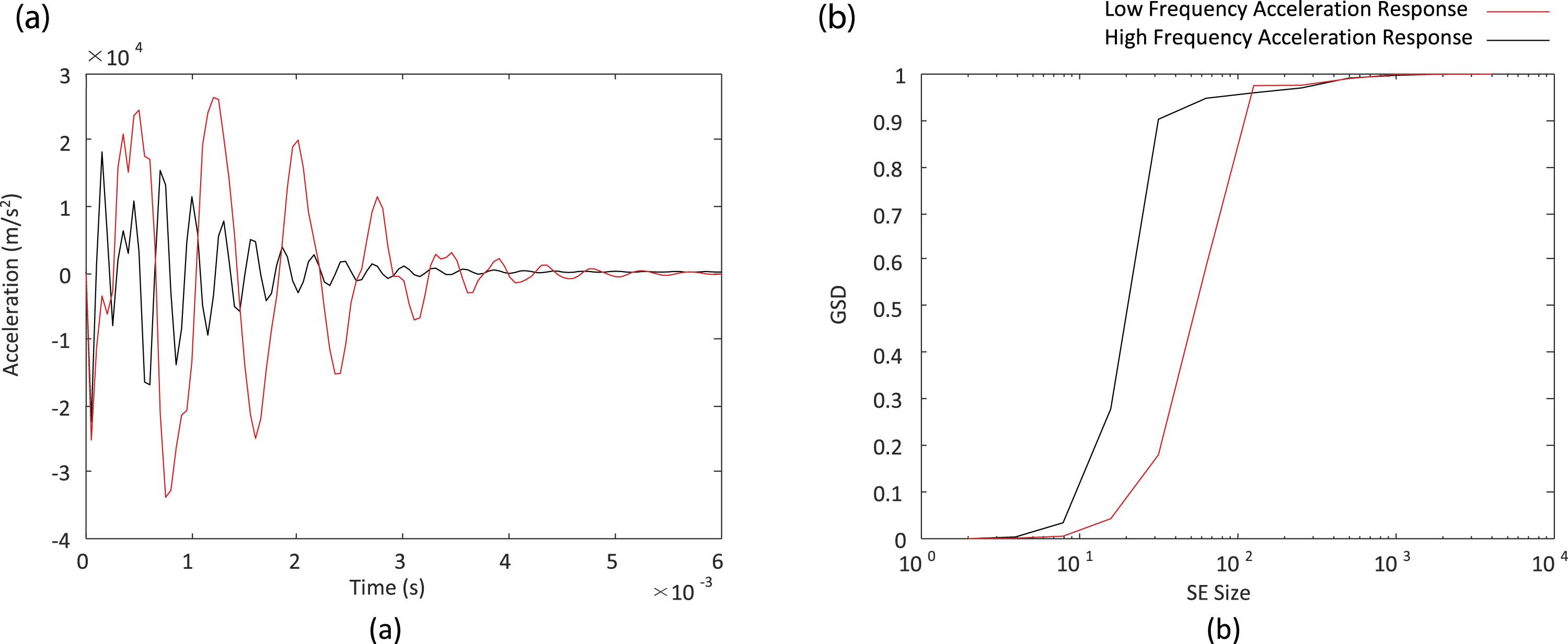

As can be seen in Figure 4, the GSD significantly reduces the dimensionality of the acceleration time history curves. The dimensionality of the time series data is the acceleration response of the beam, measured at 121 time points, whereas the GSD curves consist of the amount of data captured over 11 SE sizes. This reduction allows the computation required to find the distance between each curve in the dataset and compute the resulting clusters to be significantly reduced.

Clustering methodologies

GSD curves were generated from the acceleration response of the systems, and clustering methodologies were applied to find any underlying structures in the dataset now represented by the GSDs. Multiple clustering methodologies were applied to the data including PAM, k-means, and agglomerative hierarchical clustering. All the clustering methodologies were evaluated based on an average silhouette value. The silhouette analysis work by measuring the distance between all the datapoints in a given group, and assigning a datapoint a value between −1 and 1 based on that distance. A silhouette value of −1 would indicate that the datapoint has been incorrectly clustered, while a 1 would indicate that the cluster is appropriate. An average silhouette value is taken for all of the datapoints to validate the grouping. ²¹ Once the average silhouette value for each number of clusters is known, a scree plot can be generated. An example scree plot is shown in Figure 5.

Figure 5.

Scree plot for the partitioning around medoids algorithm clustering method.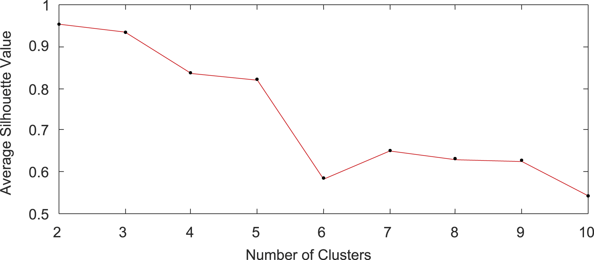

Also of interest for the grouping is looking at the acceleration curves to see if the grouping actually caries any physical significance. For the PAM algorithm, and multiple other algorithms tested (k-means, CLARA, and other variations of PAM), the physical significance of the clusters was not seen to be clear. The final clustering methodology applied that did yield the desired results was an agglomerative hierarchical clustering technique. The agglomerative hierarchical clustering techniques works by using a “bottoms-up” approach, placing each datapoint into its own cluster, then combining it with the next closest cluster. The process continues until the specified number of clusters is met. ²¹ Again, multiple numbers of groups were tested, and both the silhouette values as well as the physical significance of the clusters was evaluated. In the end, this method yielded the most promising results.

Development of the artificial neural network

Once an adequate GSD model was in place, the ANN was developed. The goal for the ANN was to be able to input the same parameters as the original finite element model (length, width, coefficient of friction, and magnitude of pressure loading) and be able to output an acceleration time series prediction of the system response. In developing the ANN, the number of hidden layers and number of neurons in each layer was investigated to find out if there was any significant benefit in using a Deep Learning Neural Network. A thorough investigation regarding the underlying neural network architecture was performed. The results showed that two hidden layers with eight neurons each was one of the best performing architectures further discussed in the results section of this article. The activation function used for the two layers was the sigmoid activation function, and the cost function used was the cross-entropy function. It should be noted that factors that affected the training time was the randomization of the starting weights to assure robustness, and the cost function employed.

The neural network structure optimization was performed by running a test on multiple neural network structures. Each of these tests involved training a single neural network 100 times and collecting performance measures which include network cost, mean squared error, mean absolute error, root mean squared error, and mean absolute percentage error. These performance measures were then averaged and analyzed. The result of this test showed that two hidden layers with eight neurons each achieved a balance between minimizing multiple metrics while avoiding diminishing returns. The resulting topology of the ANN is shown in Figure 6.

Figure 6.

Topology of the final artificial neural networks (ANNs).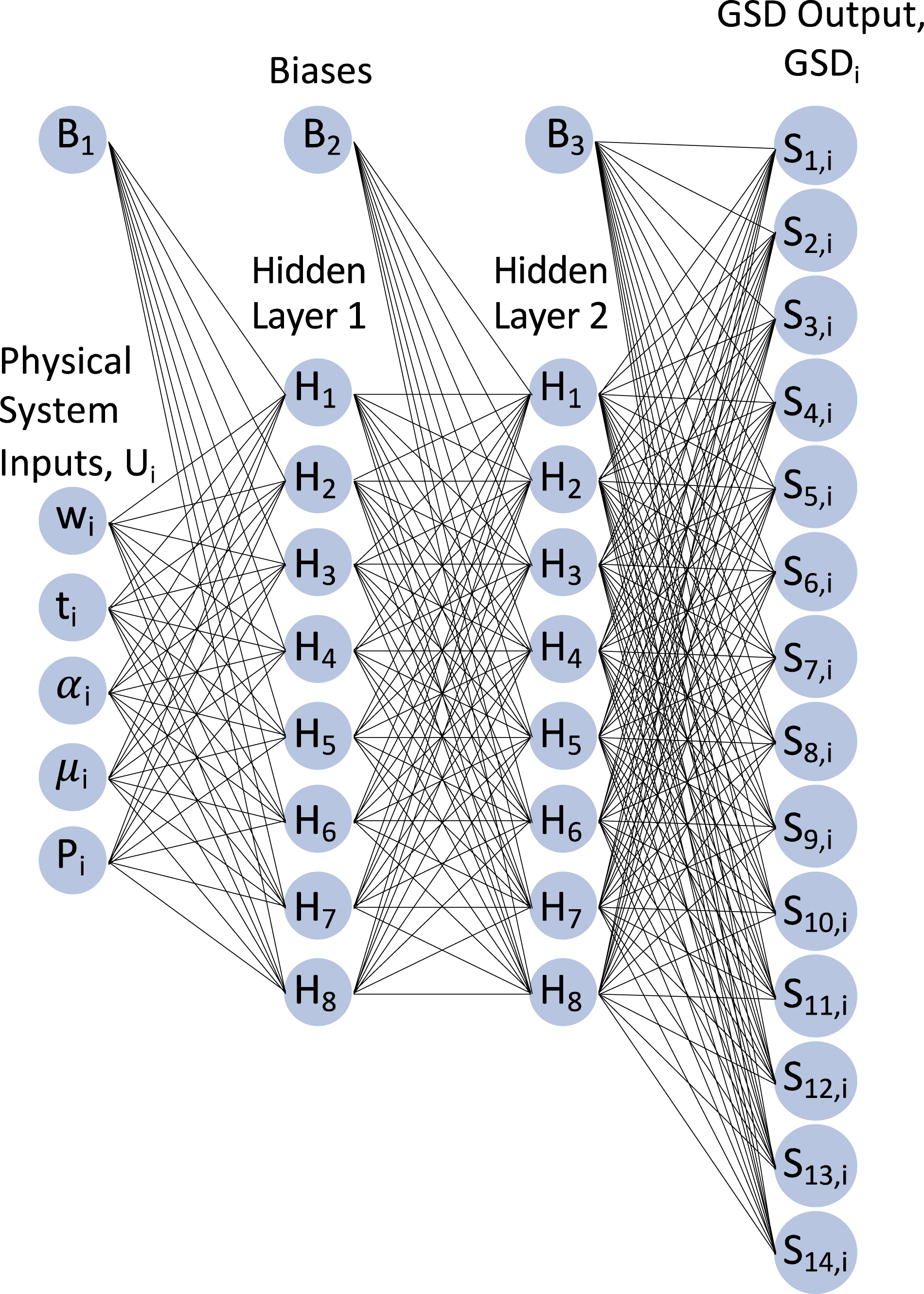

To train and validate the model, the original set of 200 curves was split into a 20% sample for model testing and validation. These 40 curves were chosen at random (20%), and the remainder were used in the training set. The final goal of this research was for the GSD that was output by the ANN to be converted back into an acceleration curve and compared to the one output from the FE model. Although more sophisticated methods of representing the time series response from a GSD are under investigation, as a first step in making acceleration response predictions for comparison with the actual structural response (or model in this case), the predicted GSD was clustered with the GSD clusters developed during model training. A characteristic acceleration curve from the relevant cluster was then used as the predicted acceleration curve. This characteristic curve was selected by finding the existing GSD that matched closest with the GSD curve generated by the neural network. This process is illustrated in Figure 7.

Figure 7.

(a) ANN produced GSD. (b) Closest existing GSD. (c) Acceleration curve corresponding to GSD in (b).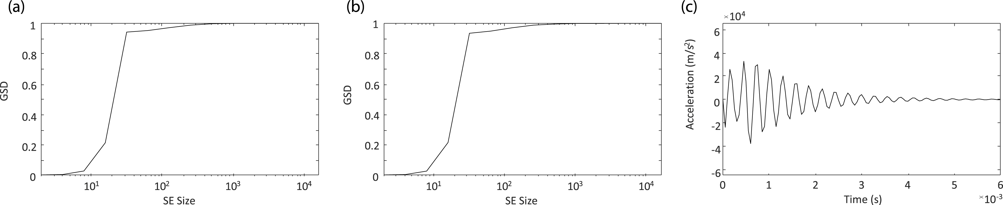

Using this process, the methodology allows neural net produced GSDs to relate back to existing acceleration responses.

In conclusion, the overall step procedure for the final ANN model methodology is as follows:

For each set of physical characteristic parameters, an acceleration curve is generated. Let U_i be the set of physical system characteristics consisting of w_i, t_i, $\alpha$ _i, $\mu$ _i, and P_i used to generate an acceleration curve A_i.

For each A_i, a corresponding GSD_i was created consisting of sieve sizes S_1,i through S_14,i.

Clustering of all GSD_i was done using hierarchical clustering.

Based on the clusters, an ANN was trained to take inputs U_i and output GSD_i.

After training, the ANN can predict each GSD_k from a new set of physical parameters U_k. Once a new GSD_k is found, a nearest neighbor approach is used to determine which predetermined cluster the new GSD_k belongs to and which known acceleration curve A_i within the cluster it is closest to.

Thus, from a new set of physical system characteristics, a GSD is predicted from the ANN which allows to define the nearest neighbor acceleration curve, completing the process of making predictions about the dynamic response of a structure using an ANN instead of a physics-based model.

Results

The final results are based on acceleration time histories collected at the midspan of the beam. The acceleration response at the end of the beam also could have been chosen as it would not affect the methodology used; however, it could yield different results due to the configuration of the cantilever beam. Some runs resulted in little to no acceleration at the end span, which makes the use of the mid-span acceleration data justified. The best overall clustering method was found to be the hierarchical clustering method that split the GSD curves into eight distinct groups. The original clustering of the data was conducted on the entire dataset of 200 curves. Figure 8 shows the resultant eight groups of GSD curves.

Figure 8.

The clustering of the GSD curves created from the mid-span beam acceleration data.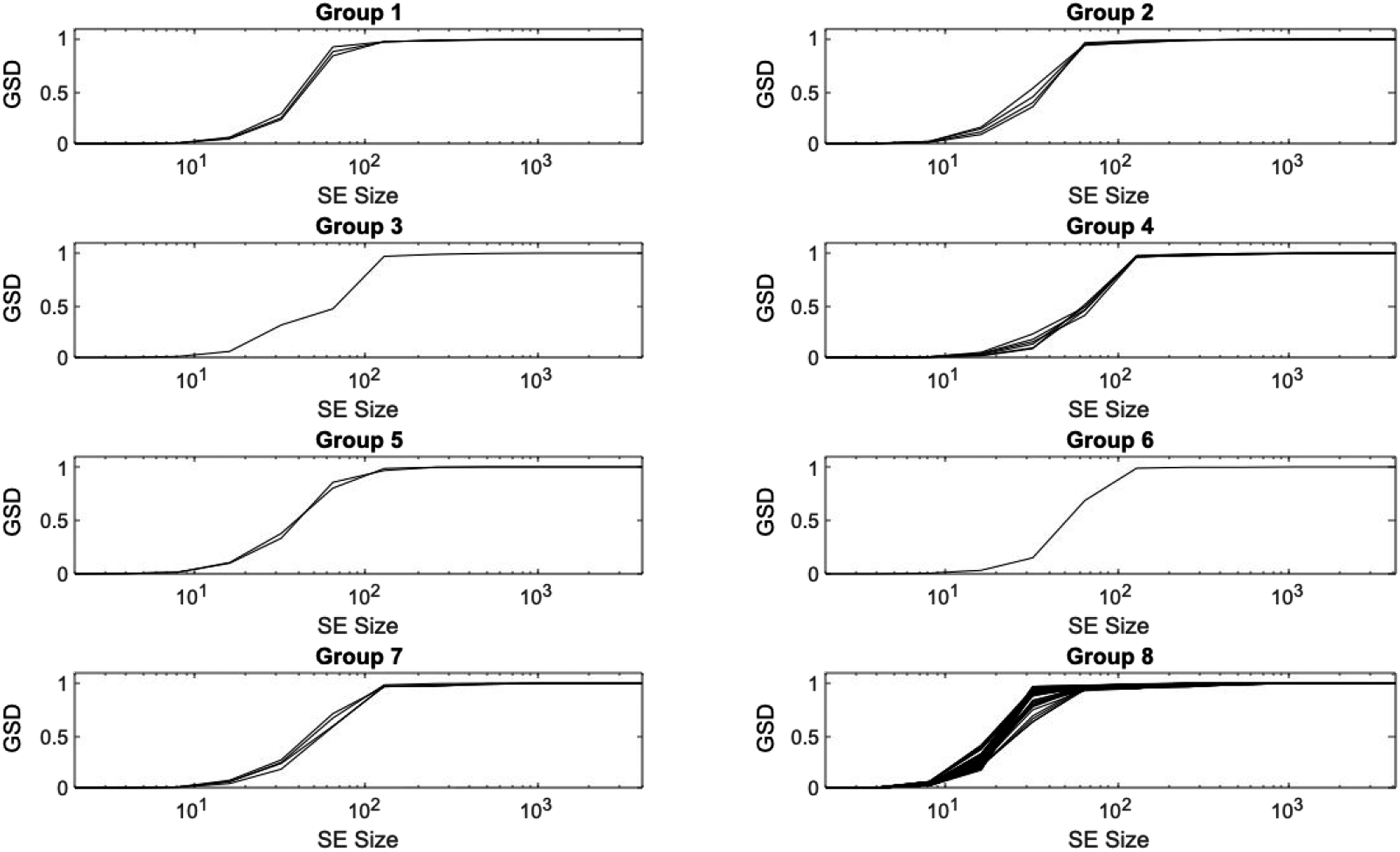

To evaluate the effectiveness of the clustering methodology used, silhouette values were used. Figure 9 shows the silhouette values for this hierarchical method for clustering.

Figure 9.

Silhouette values for the hierarchical clustering method.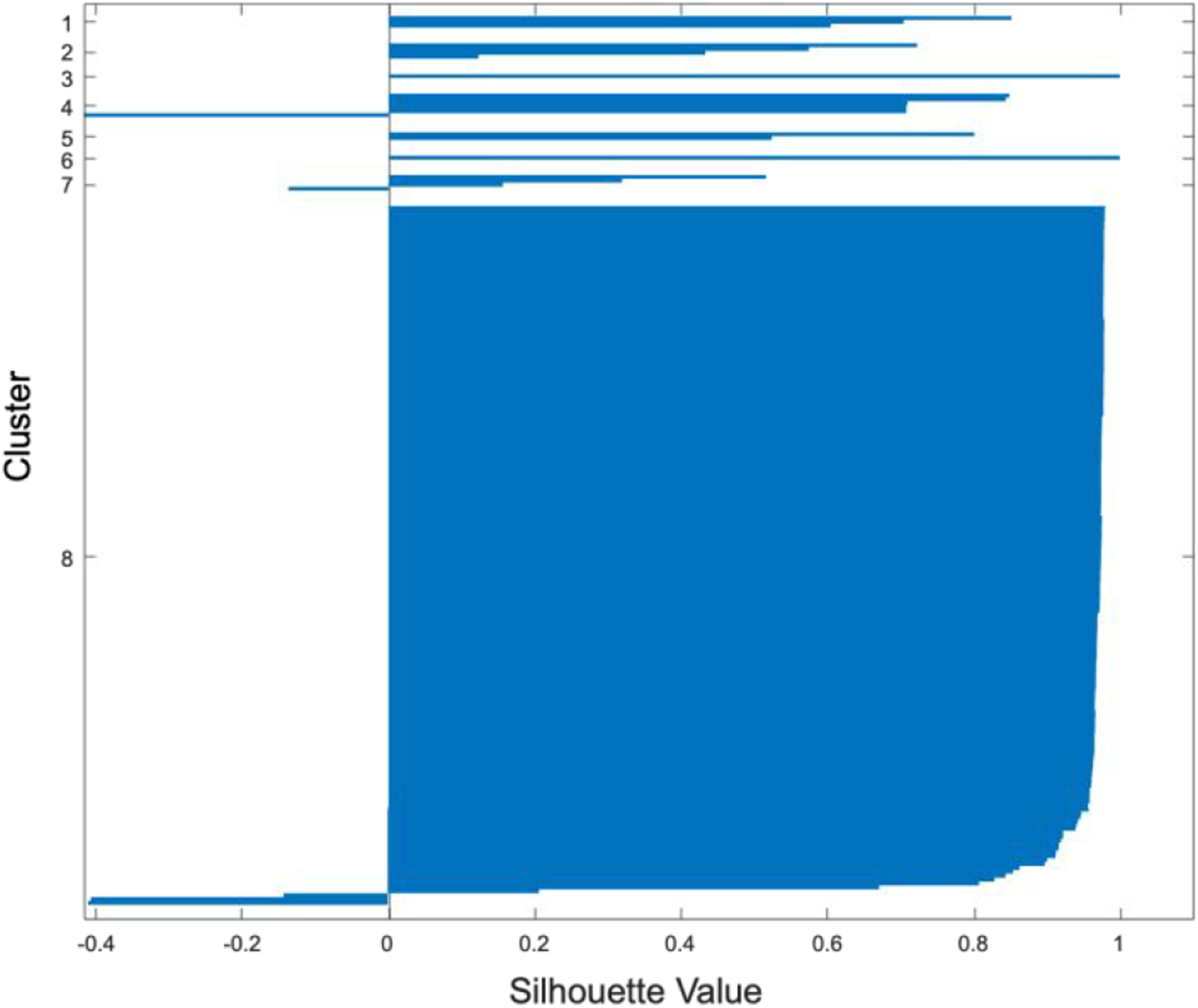

The average silhouette value for the hierarchical clustering method shown was 0.89, showing that the grouping was conducted well. However, this was not the highest silhouette value observed among other clustering methods, and some curves are still showing that they are being grouped incorrectly. Purely looking at the GSDs and silhouette values, though, gives little information on the physical properties of these groups. The corresponding grouped acceleration curves are shown in Figure 10.

Figure 10.

Acceleration curves clustered using a hierarchical method.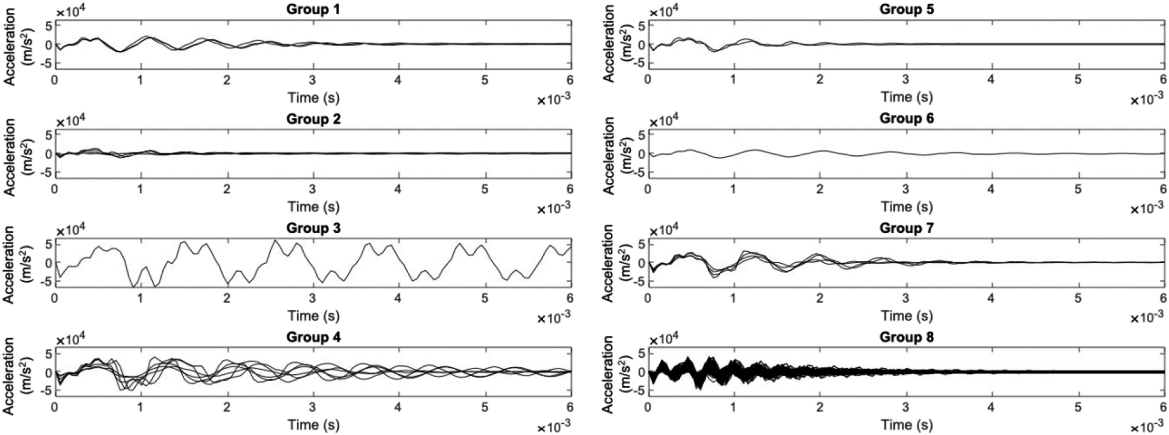

The grouped acceleration curves shows the physical characteristics of these groupings, and further shows that the grouping is, in fact, appropriate. Group 8 was the largest group by far, containing 179 of the 200 curves, and showing behavior of high frequency, high amplitude acceleration that damps out relatively quickly comparatively with the other groups. Group 3 and group 6 contain only one curve each. Group 3 contains one curve that is significantly different from the rest, a large amplitude, double-peaked oscillation that does not damp out over the analysis window. This simulation had a very high applied pressure of 6.7 MPa, and a low coefficient of friction between the wall and the beam with a value of 0.0019. This combination led to the high amplitude of accelerations observed in the output time series. Overall, the clustering methodology seems to group the acceleration curves appropriately.

These results proved positive for the GSD clustering methodology being explored in this study. By converting the acceleration time series into representative GSD curves, the data can be effectively clustered, and underlying structures in the data can be found. Next, the previously trained ANN was used to output a representative acceleration curve from the validation dataset, to be compared to the acceleration from the model generated response.

To complete this process, the ANN was trained on 190 of the original 200 datapoints, setting aside 10 for the ANN to produce and compare to the original model. The 10 GSDs output by the ANN were re-clustered into the existing dataset. This was done by finding the existing GSD that had the smallest Euclidean distance from the GSD produced by the ANN. That existing GSD that most closely resembled the ANN-produced GSD indicated the appropriate group number as well as a representative acceleration response for the ANN-produced GSD. This allowed the final comparison of the ANN methodology proposed in this study to the traditional method for modeling the dynamic behavior of structures: the finite element method. The results from this process are shown in Figure 11. Included in the figure are the mean absolute percent error (MAPE) between each of the two curves for comparison.

Figure 11.

The characteristic acceleration curves from the ANN compared to the actual acceleration curves.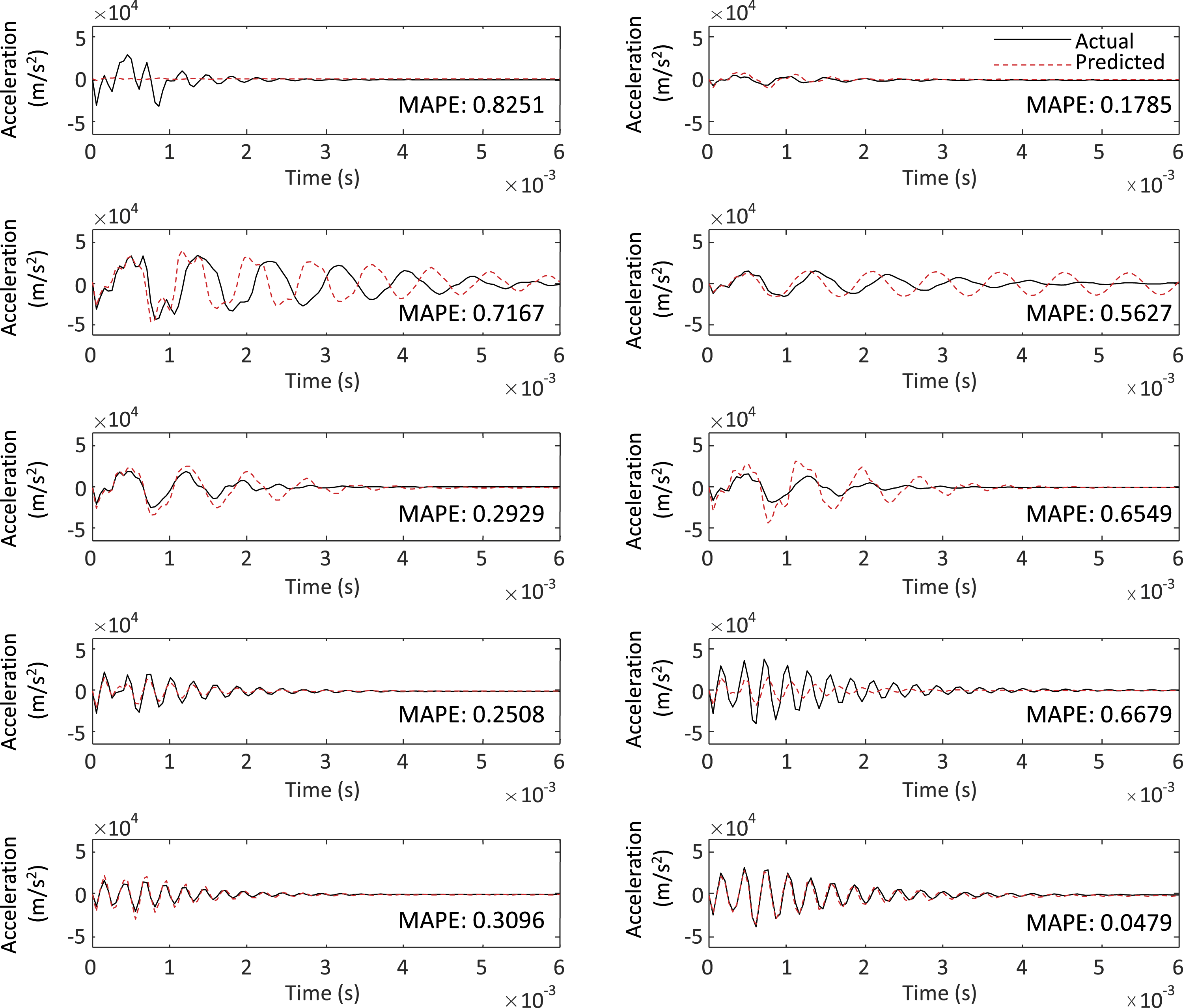

The figure shows that all the characteristic acceleration curves have fairly low MAPE values, under 1%; however, in some cases the MAPE does not accurately represent the differences between the two curves. For example, for the two curves with a MAPE of 0.7167, the curves clearly have very similar shapes and amplitudes, the characteristic curve having an amplitude of $1.5\times {10}^6$ m/s², while the actual had an amplitude of $1.3\times {10}^6$ m/s². On other curves, it is clear that the frequency is captured quite well, but the amplitude is not, as in the case for the curves with MAPE 0.6679, whose amplitudes match poorly ( $0.6\times {10}^6$ m/s² predicted versus $1.5\times {10}^6$ m/s² actual), but whose frequencies matched much more closely. The natural frequency of the predicted response being 3.47 kHz, while the actual response had natural frequency 3.8 kHz. This particular case illustrates one downside of the GSD, its inability to capture amplitude information for the time series data, which can lead to poor predictions like this one.

Although these preliminary results approximate the acceleration response better in some cases than in others, the methodology developed to make predictions about the acceleration response of a nonlinear dynamic system is clearly promising. In most cases the amplitude, frequency and damping of the system is well captured. It is also worth noting that although the goal of the finite element model was simplicity and tractability, the ANN model produces results in approximately 1/100th of the time it takes the physics-based model using comparable computational resources.

Conclusion

The methodology developed in this study utilized a nonlinear structural model to produce acceleration responses for systems with varying geometries, loading conditions, and material properties. Mathematical morphology tools were then used to convert acceleration time history curves into lower dimension curves known as GSDs. Clustering methodologies were then applied to these GSD curves to find underlying structures in the dataset that could not be completed using the acceleration time history data. These clusters and the GSDs were then utilized to train an artificial neural network (ANN) that could take inputs from the original nonlinear model and create a GSD. The GSDs output by the ANN were re-clustered, and a representative acceleration time history curve was produced.

The final implementation of the methodology showed promising results. One result was that the GSD proved to be an effective way to decrease the dimensionality of acceleration time history data while still retaining information about the physical characteristics of the original system. This was made evident by the clearly distinguished acceleration response clusters produced by clustering the GSD (Figure 9). Second, the ANN was proven to be able to effectively produce GSD curves that still reflected the inputs of the nonlinear system. Of the ten GSDs produced, nine of them re-clustered into the same groups as the actual GSDs. Also, comparisons of representative curves from the ANN model to actual acceleration curves from the FE model showed values of MAPE as low as 0.1785 with very similar frequency responses. This result showed that the ANN could be a reliable surrogate model for FE simulations. A methodology such as the one developed here could be applied to acceleration data of a structural system, and the ANN used to make predictions on the response of the system for other loading environments in place of computationally expensive physics-based modeling tools. With a larger dataset (such as could be found from testing data or from in-use structural monitoring), the quality of predictions would likely increase as well as refining the set of physical systems characteristics that improve the resulting acceleration curve.

These results could directly benefit the field of civil engineering, specifically structural dynamics, as it presents a surrogate model to FE simulations for efficiently obtaining results from a structural dynamic model. This methodology could be used directly with actual dynamic data from a structure of interest, providing a computationally efficient model that would reduce both modeling and testing time and resources. It also proves to be an efficient method for reducing dimensionality of time series data, allowing clustering methodologies to be used. These clustering methodologies allow unseen characteristics of the system to be readily obtained rather than searching through the data manually.

Plans for future work include the development of a more sophisticated methodology for converting GSDs back into acceleration curves. In addition, the application of the methodology to test data in place of a simplified computational model is also being investigated to further confirm the validity of the approach.