
Abstract
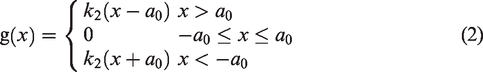
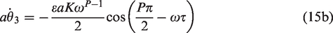
The forced vibration of a single-degree-of-freedom piecewise linear system containing fractional time-delay feedback was investigated. The approximate analytical solution of the system was obtained by employing an averaging method. A frequency response equation containing time delay was obtained by studying a steady-state solution. The stability conditions of the steady-state solution, the amplitude–frequency results, and the numerical solutions of the system under different time-delay parameters were compared. Comparison results indicated a favorable goodness of fit between the two parameters and revealed the correctness of the analytical solution. The effects of the time-delay and fractional parameters, piecewise stiffness, and piecewise gap on the principal resonance and bifurcation of the system were emphasized. Results showed that fractional time delay occurring in the form of equivalent linear dampness and stiffness under periodic variations in the system and influenced the vibration characteristic of the system. Moreover, piecewise stiffness and gap induced the nonlinear characteristic of the system under certain parameters.
Introduction
As a branch of nonlinear dynamics, nonsmooth systems extensively exist in engineering applications, including circuits,1,2 vehicle suspensions,3,4 and vibration isolators. 5 Each piecewise system in nonsmooth systems is linear and can be easily processed, while the global solution of the system cannot be obtained under most circumstances.6–8 Moreover, many complicated dynamic phenomena are generated due to the existence of gaps, which may exert adverse effects on the system. Hence, piecewise linear systems have attracted increasing research attention. Shaw and Holmes 9 used a central manifold theorem to analyze the local bifurcation of a piecewise linear impact oscillator under simple harmonic excitation force and studied chaotic motion under homoclinic transverse conditions. Hu10,11 found that the nonsmoothness of the vector field in a continuous piecewise linear system destroys the second-order differentiability of Poincare mapping at a fixed point and thus results in system singularity. Luo 12 analyzed all kinds of unstable and stable periodic motion morphologies of a piecewise linear system under periodic excitation. Jin and Guan 13 evaluated the stability of the periodic motion of an asymmetric piecewise linear model with multiple degrees of freedom. The selection of proper piecewise stiffness or dampness can improve the performance of the original dynamic system by improving the stability and buffer performance of the system.14–16
Based on the extensive application of fractional calculus and interdisciplinary development, fractional calculus has appeared in models in numerous disciplinary fields and practical problems,17–19 such as the fractal Micro-Electro-Mechanical System (MEMS) and Toda oscillators. Zuo 20 designed a gecko-inspired fractal‑like receptor system for the three-dimensional printing process. He et al. 21 investigated the possible working mechanism of ink slab-like materials by using two-scale fractal derivatives. Given that fractional models can effectively describe essential system characteristics,22–24 an increasing number of studies have been conducted on fractional order. Moreover, studies on fractional differential systems have achieved considerable progress, especially in the analysis of the equilibrium points of systems, quantities of periodic solutions, limit cycles, and stability.
However, in actual systems, particularly control systems, the time-delay phenomenon is ubiquitous in various fields, and time delays usually lead to changes in vibration form and system instability or oscillation. Even simple systems become unstable when time-delay factors are neglected in the modeling process. Time delays also cause difficulties in the theoretical analysis of systems. 25 The analysis of systems with time delays is imperative in studying actual systems, particularly control systems. Therefore, systems with time delays, especially fractional systems with time delays, should be investigated comprehensively.
Integer-order systems with time delays have been extensively investigated, but fractional systems with time delays have been largely ignored because of their complexity.26,27 With regard to the control of fractional systems with time delays, Kaslik and Sivasundaram and Li and Zhang28,29 conducted a stability study on a fractional linear system with time delay. Deng et al. 30 investigated the stability of a linear fractional differential system with multiple time delays. Babakhani et al. 31 determined a solution for the fractional differential equation with time delay and hope bifurcation. Ye et al. 32 also determined a positive solution for the fractional differential equation with time delay. Zhang 33 proved that for a specific type of a fractional system with time delay, sufficient conditions for stability within finite time can be obtained. Čermák et al. 34 studied the stability and progressivity of the fractional differential equation with time delay.
A few studies have controlled piecewise smooth systems by using fractional time-delay feedback. The dynamic behaviors of fractional time-delay feedback systems became complicated due to the existence of nonlinear factors caused by piecewise stiffness. Steady-state solutions, system stability, and the effects of all kinds of system parameters on dynamic system characteristics are yet to be studied comprehensively.
The fractional time-delay feedback of a single-degree-of-freedom (SDOF) piecewise linear system was studied in the current work. An averaging method was used to analyze the approximate analytical solution of the system and obtain the principal resonance amplitude–frequency response equation with time-delay parameters and stability conditions of the system. The effects of time-delay and fractional differential parameters and gaps on the principal resonance and bifurcation of the system were investigated in detail through a numerical analysis.
Model of system dynamics and approximate solution
The SDOF piecewise linear oscillator with fractional time-delay feedback mentioned in this study consists of a mass block, external excitation, linear spring, linear dampness, and fractional time-delay feedback term. Its physical model is shown in Figures 1 and 2.

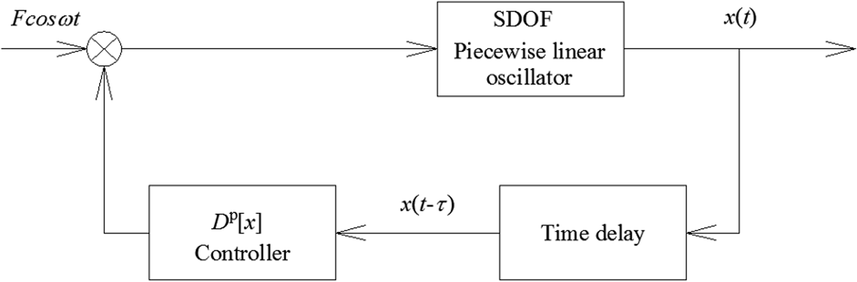
Fractional time-delay feedback of the piecewise linear oscillator. SDOF: single-degree-of-freedom.
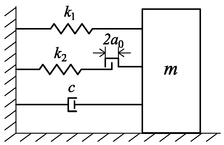
SDOF piecewise linear oscillator.
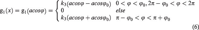
Many analytical methods, such as fractional complex transform, 38 variational iteration, 39 homotopy perturbation method, 40 and He’s frequency method, 21 could be used for the fractional differential equation as shown in equation (1).
The following parameters are introduced.

Equations (1) and (2) can be transformed as follows

The principal resonance of the system was studied.

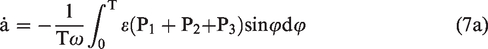
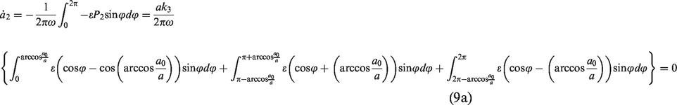
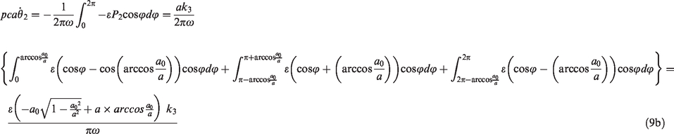
In accordance with the averaging method,
Then

Equation (5) can be organized as follows


According to the averaging method

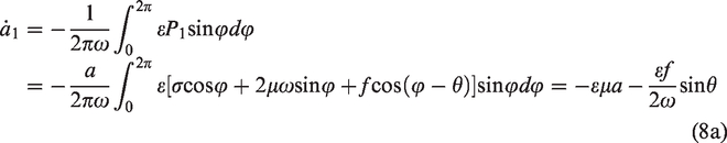
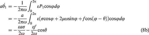
The following equation is obtained in accordance with the Caputo fractional differential definition.
41
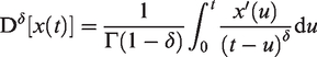
Then
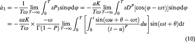
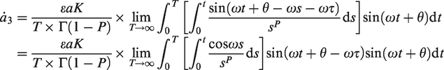


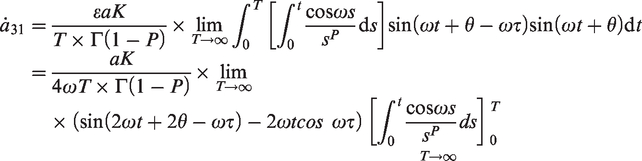
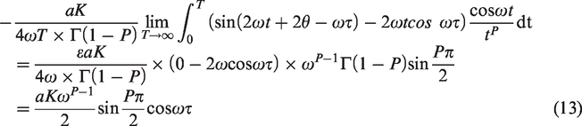
After the integration of the parts and fractional order calculation in equation (12), the first part of the integral in equation (11) is expressed as follows
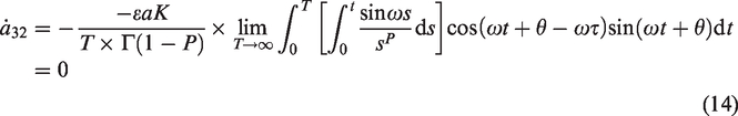
Similarly, the second part of the integral in equation (11) is expressed as follows
Hence

The process is repeated, and the following expression is obtained.
In sum

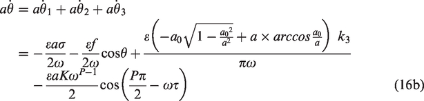
The following expression can be obtained by substituting the original parameters


Steady-state solution and its stability conditions
The steady-state solution of the system was analyzed,


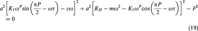
The trigonometric function term was eliminated, and the amplitude–frequency response equation containing the time delay in the system was obtained through the simplification
The stability of the steady-state solution was analyzed.
Linear processing of equation (18) was performed to obtain the differential equations of two disturbing quantities,


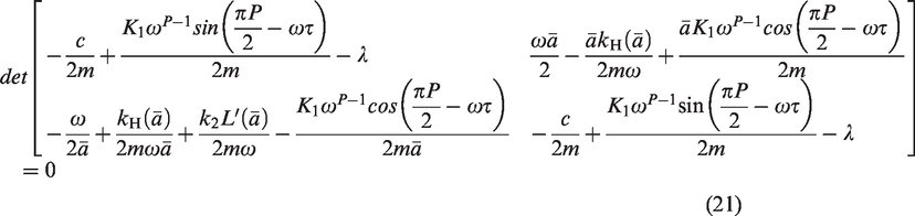
Equation (20) was manipulated and simplified, and the following expression was derived.

The stability condition of the steady-state solution of the system was obtained through equation (22).


Numerical verification
To verify the correctness of the steady-state solution obtained previously, we compared the solution of the amplitude–frequency equation (19) and the result obtained through the numerical simulation of equation (1). The selected parameters were as follows: m = 5, k1=5, k2=6, c = 1, p = 0.5, K1=5, F = 2, and a0=0.8.
To analyze the effects of time delay on the amplitude–frequency curve, we selected two time-delay values for comparison:


In the calculation process, the time step was set to h = 0.004, and calculation time was set to 500 s. The average value of the last 10% of the maximum response values was interpreted as the steady-state response amplitude. The numerical calculation results at
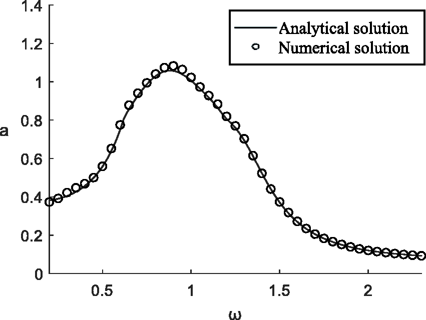
Comparison of analytical and numerical solutions at τ = 5.2.
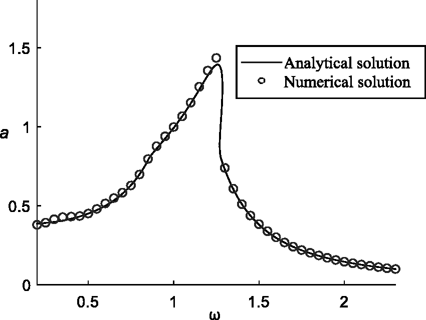
Comparison of analytical and numerical solutions at τ = 0.5.
Figure 3 shows a comparison of the numerical and analytical solutions at
Effects of system parameters on the vibration response
Effects of time delay on steady-state solution amplitude and time-delay response
Figures 5 and 7 show the response time delay–amplitude relation curves of the steady-state solution of the system under different excitation frequencies.
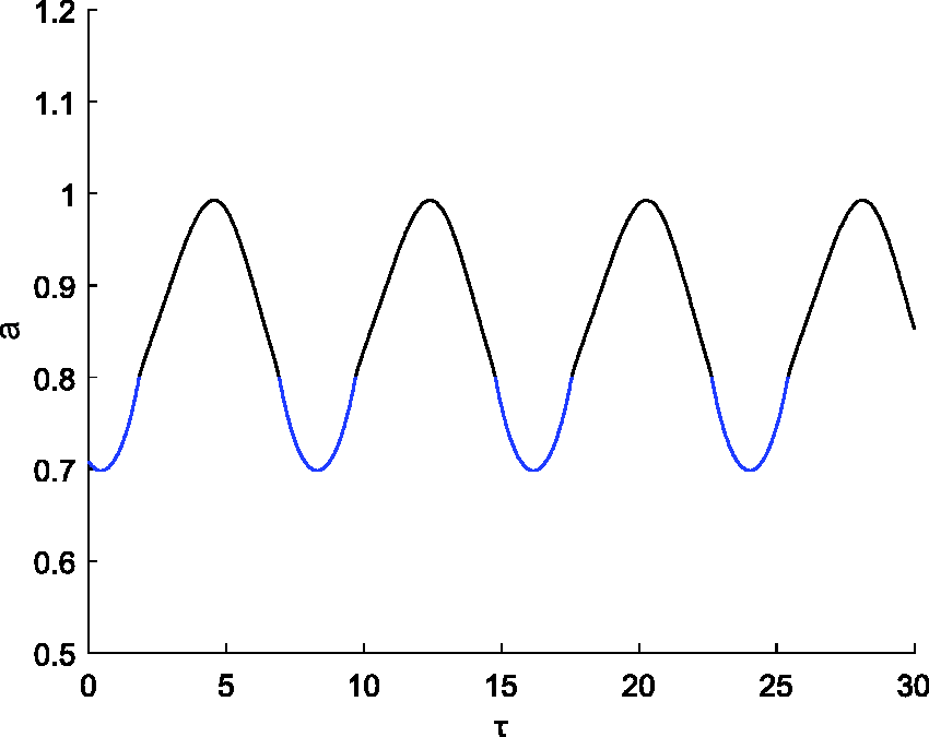
Time delay–amplitude relation chart of the steady-state solution of the system (m = 5, c = 1, F = 2, k1=5, k2=10, a0=0.8, K1= –1, p = 0.5, ω = 0.8).
Figure 5 shows the response time delay–amplitude relation chart of the steady-state solution of the system under excitation frequency ω = 0.8. As the time delay increased, the system response amplitude presented a periodic change, which was obviously caused by the trigonometric function related to the time delay in equation (18). Figure 5 also shows that for the gaps of the piecewise system, the time-delay change caused a continuous change in the vibration response between the vibration amplitude, which is smaller than the gap value (solid blue line), and the system, which is higher than the gap value (solid black line) in each period of time delay-dependent amplitude change. Hence, when the other conditions are fixed, the system vibration mode can be changed by regulating the time delay.
Figure 6 shows the response time delay–amplitude relation chart of the steady-state solution under excitation frequency ω = 1.27. When the external excitation frequency increased, the system dynamic response became increasingly complicated under the dual effects of piecewise nonlinearity and time delay, and the situation shown in Figure 6(a) occurred. Multiple solutions appeared in the time delay-dependent change of the system response amplitude and triggered piecewise stiffness. Moreover, no response curve with piecewise stiffness can be observed in Figure 6(b). The system response with time delay is a linear curve presenting a periodic change without piecewise stiffness. Hence, this multisolution phenomenon is a nonlinear phenomenon induced by the piecewise nature of the system.
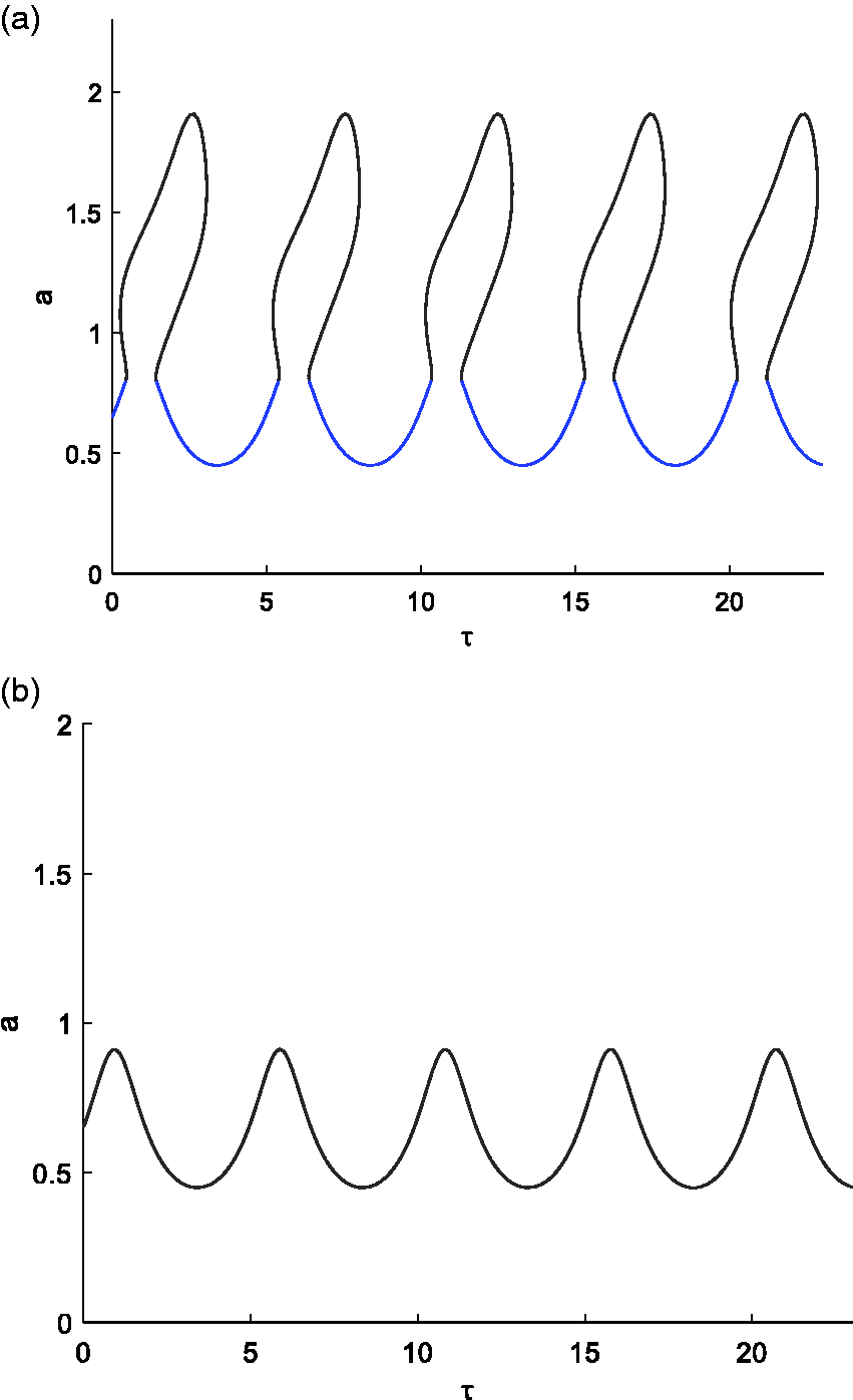
(a) Time delay–amplitude relation chart (with piecewise stiffness) of the steady-state solution of the system (m = 5, c = 1, F = 2, k1=5, k2=10, a0=0.8, K1= –1, p = 0.5, ω = 1.27). (b) Time delay–amplitude relation chart of the steady-state solution of the system (without piecewise stiffness) (m = 5, c = 1, F = 2, k1=5, k2=10, a0=0.8, K1= –1, p = 0.5, ω = 1.27).
With the continuous increase in external excitation, the topological structure of the time delay-dependent change curve of the system response amplitude underwent a major change. Figure 7 shows the change curve of a-
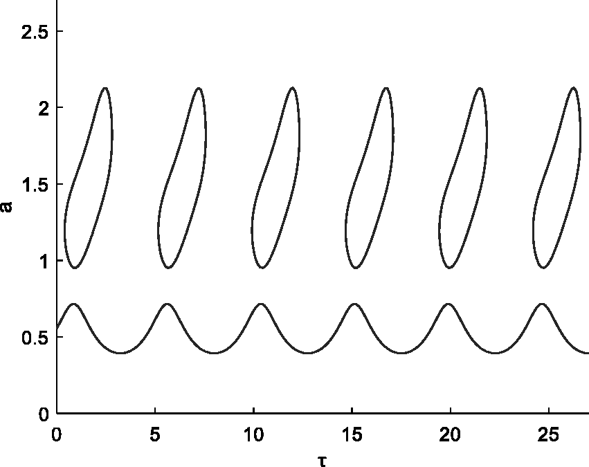
Time delay–amplitude relation chart of the steady-state solution of the system (m = 5, c = 1, F = 2, k1=5, k2=10, a0=0.8, K1= –1, p = 0.5, ω = 1.32).
In summary, the system vibration response presented three states under different excitation frequencies. The vibration responses under the three states exhibited time delay-dependent periodic changes, and the period duration was decided by excitation frequency. For a simplified analysis, the most typical state shown in Figure 6 was considered for evaluation in the subsequent investigation of the effects of other system parameters on the system vibration response.
Effects of piecewise parameters on the amplitude–time delay response of the steady-state solution
The effect of piecewise stiffness on the system vibration characteristic was first analyzed. Figure 8 shows the vibration amplitude–time delay relation curve of the steady-state solution under k2=0, 6, 8, and 10. When k2=0 and piecewise stiffness was absent, the system vibration amplitude presented a complete linear characteristic and gradually increased with k2. When k2=6, 8, and 10 and the system presented a nonlinear vibration characteristic, the system jump amplitude increased with k2, indicating that the system nonlinearity was gradually enhanced. As the contribution of piecewise stiffness to system stiffness continuously increased, the peak response amplitude gradually decreased, but the system response period did not change.
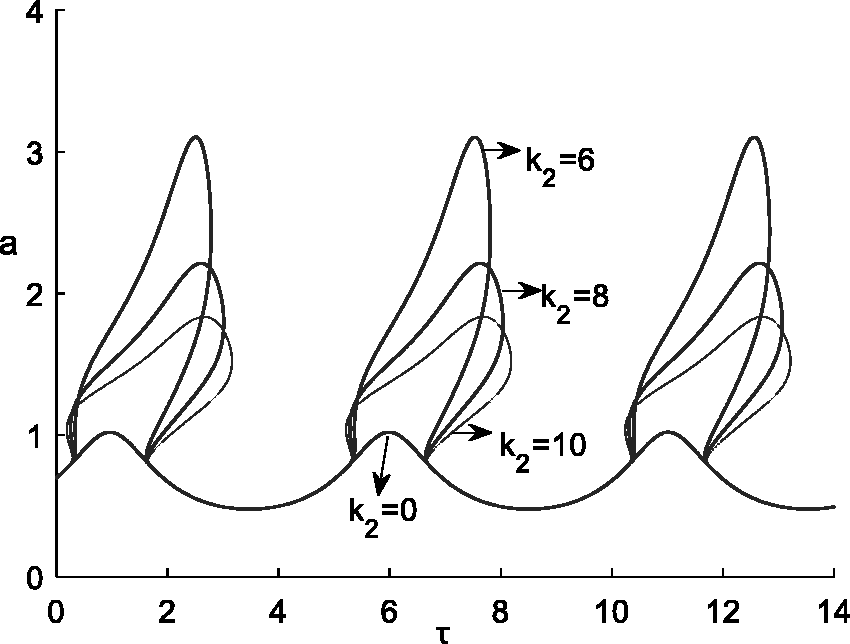
Graph of the effect of piecewise stiffness on the amplitude–time delay relation of the steady-state solution (m = 5, c = 1, F = 2, k1=5, a0=0.8, K1= –1, p = 0.5, ω = 1.25).
Figure 9 shows the amplitude–time delay relation chart of the steady-state solution of the system under fractional orders 0.1, 0.5, and 0.9. When fractional order p increased, the amplitude response curve of the steady-state solution became skewed toward the direction of the increase in time delay, and the peak response amplitude was gradually enlarged, which can also be explained by equation (17). We considered the weakening effect of the equivalent stiffness generated by the fractional time-delay feedback term on system stiffness and the resulting periodic change. The peak response amplitude of the system within a period gradually increased with p.
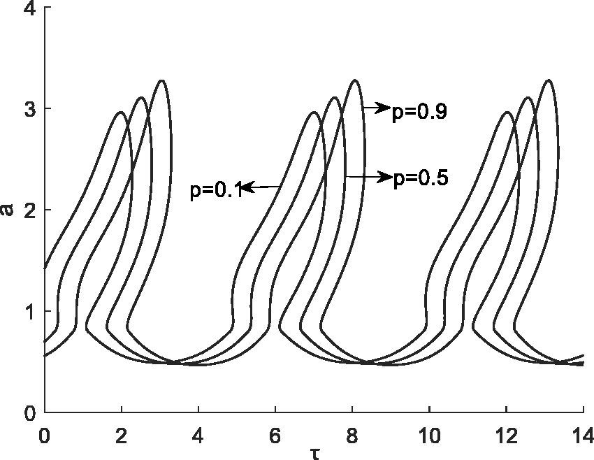
Graph of the effect of fractional order on the amplitude–time delay relation of the steady-state solution (m = 5, c = 1, F = 2, k1=5, k2=6, a0=0.8, K1= –1, ω = 1.25).
The response amplitude–time delay relation curve obtained through equation (19) under K1 = −0.4, −0.7, and −1 is shown in Figure 10. When K1 gradually increased, the resonance amplitude of the system was gradually enhanced because the damping effect of the fractional time-delay term on the system weakened step by step. Given that the equivalent linear stiffness generated by the fractional time-delay term to the system gradually weakened, the nonlinear characteristic of the system also gradually weakened, and the nonlinearity was stronger under K1= −0.4 than under the two other circumstances with the islanding phenomenon.
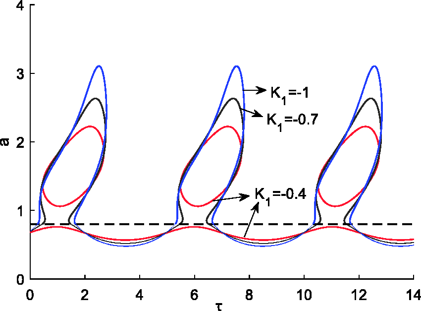
Graph of the effect of fractional coefficient on the amplitude–time delay relation of the steady-state solution (m = 5, c = 1, F = 2, k1=5, k2=6, a0=0.8, p = 0.5, ω = 1.25).
Effects of piecewise parameters on the amplitude–time delay response of the steady-state solution
Figure 11 shows a graph of the effect of the piecewise gap on the amplitude–time delay relation of the steady-state solution. When a0 was small and the system presented a linear vibration, vibration occurred at the position beyond the gap. When a0=0.5, the system presented a nonlinear vibration mode. Although the curve period did not change, the time-delay value corresponding with the peak amplitude changed, and the peak response amplitude increased. As a0 increased, the topological structure of the system response curve would change with the islanding phenomenon, indicating that the system nonlinearity was continuously enhanced. However, the trajectory of the linear vibration part overlapped with that under a0=0, and the peak response amplitude continued to increase. In general, the change in the a0 value enhanced the system nonlinearity and increased the peak response amplitude. Moreover, the time delay corresponding to the peak amplitude changed, but the period of the periodic response amplitude remained unchanged.
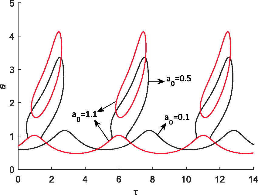
Graph of the effect graph of piecewise gap on the amplitude–time delay relation of the steady-state solution (m = 5, c = 1, F = 2, k1=5, k2=6, K1= –1, p = 0.5, ω = 1.25).
Singularity analysis
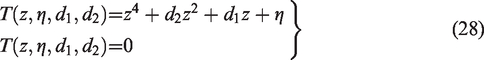
To further study the frequency response characteristics of the fractional-order primary resonance of the piecewise system, we applied singularity theory to analyze the bifurcation of the system and determine the influence of the system parameters on the response characteristics of the fractional-order piecewise system. The amplitude–frequency response equation was expanded by Taylor expansion at point


The bifurcation equations of the system are as follows
The point sets corresponding with the system were obtained through the corresponding calculation. The calculation processes are as follows The set of bifurcation points is
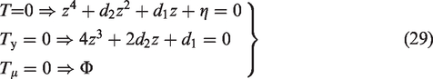
That is, the set of bifurcation points 2. The set of hysteresis points is
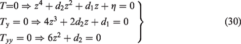
That is, the set of hysteresis points 3. The set of double-limit points is
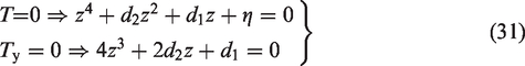
That is, the set of double-limit points 4. The set of transition points is

That is, the set of transition points
The spatial distribution of the transition sets is shown in Figure 12.
Spatial distribution of the transition sets.
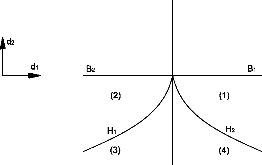
The topological structure diagrams of the bifurcation curves corresponding to different regions of the transition sets are shown in Figure 13.
Topological structure diagrams of the bifurcation curves.
Figure 13 indicates that in spatial distribution regions B1, (1), B2, and (2), the structure of the solution is one d1 corresponding to two d2. In regions H1, (3), H2, and (4), the structural form of the solution changes from one d1 value corresponding to two d2 solutions and gradually develops into the case of one d1 value corresponding to four d2 solutions.
Effects of system parameters on system bifurcation
The changes in unfolding parameters d1 and d2 affect the transition set of the system, and the change in bifurcation parameter μ affects the principal resonance response of the system. By analyzing the effects of time delay, piecewise gap, and fractional order on unfolding parameters d1 and d2 and bifurcation parameter μ, the influences of these system parameters on the bifurcation of the system were studied.
Effect of time delay on system bifurcation
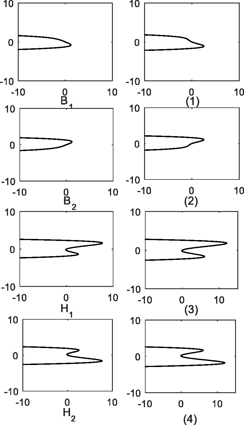
The selected parameters were as follows: m = 5, c = 1, F = 2, k1=5, k2=6, K1= –1, p = 0.5, and ω = 1.27. Piecewise gap a0 was set to 0.2, 0.4, 0.6, 0.8, and 1.0. Then, the relationship curves of unfolding parameters d1 and d2 and bifurcation parameter μ with time delay τ were drawn based on equation 28, as shown in Figure 14(a) to (c).
(a) Influence of piecewise gap a0 on unfolding parameter d1. (b) Influence of piecewise gap a0 on unfolding parameter d2. (c) Influence of piecewise gap a0 on bifurcation parameter μ.
Figure 14(a) to (c) indicates that for each given piecewise gap value, when time delay τ ≤ 0.7, the unfolding and bifurcation parameters gradually increased with the increase in time delay τ. The positions of the transition set also changed with the increase of time delay τ. The range of transition spaces (1) and (2) kept increasing, and the range of transition spaces (3) and (4) gradually decreased, indicating that the complex response areas of the principal resonance of the system gradually became small. When the time delay value was 0.7<τ < 3, as time delay τ increased, unfolding parameter d1 and bifurcation parameter μ decreased, and unfolding parameter d2 increased. Time delay τ had a much greater influence on unfolding parameter d1 than on unfolding parameter d2.
We conclude that with the increase in time delay τ, the range of transition spaces (1) and (2) continued to decrease, and the range of transition spaces (3) and (4) continued to increase, showing that the complex areas of the principal resonance responses of the system gradually widened. When time delay τ > 3, the periodic processes were repeated as time delay τ increased. Time delay τ had a much greater influence on unfolding parameter d1 and bifurcation parameter μ than on unfolding parameter d2; hence, the influence of time delay on unfolding parameter d2 could be ignored.
Effect of piecewise gap on system bifurcation
Piecewise gap a0 was set to 0.2, 0.4, 0.6, 0.8, and 1.0. Then, the change curves of unfolding parameters d1 and d2 and bifurcation parameter μ with time delay τ are shown in different colors in Figure 14(a) to (c). As the piecewise gap gradually increased, unfolding parameter d1 gradually increased, and unfolding parameter d2 gradually decreased. As piecewise gap a0 increased, the range of transition spaces (1) and (2) continued to decrease, and the range of transition spaces (3) and (4) continued to increase, that is, the complex area of the principal resonance responses of the system widened.
Figure 12 indicates that the change in piecewise gap a0 exerted a great influence on unfolding parameter d1 and bifurcation parameter μ. Therefore, when analyzing the transition set change, the influence of piecewise gap a0 on unfolding parameter d2 can be ignored.
Effect of fractional order on system bifurcation
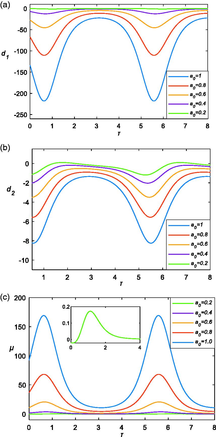
The variation relations of unfolding parameters d1 and d2 and bifurcation parameter μ with time delay τ are shown in curves of different colors in Figure 15(a) to (c) when piecewise gap a0 was 0.2, the fractional order was 0.1, 0.3, 0.5, 0.7, and 0.9, and the other parameters were unchanged.
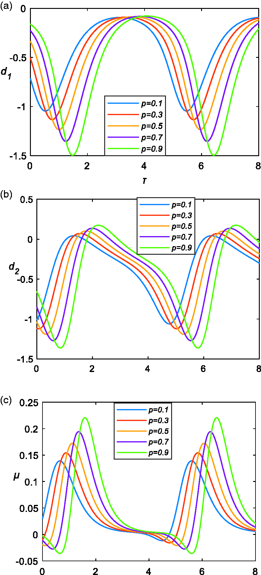
(a) Influence of fractional order p on unfolding parameter d1. (b) Influence of fractional order p on unfolding parameter d2. (c) Influence of fractional order p on unfolding parameter μ.
Figure 15(a) to (c) indicates that the change trends of unfolding parameters d1 and d2 and bifurcation parameter μ in different time-delay parameter regions varied with fractional order p. When time delay τ was in a small range, unfolding parameters d1 and d2 and bifurcation parameter μ increased with the increase in fractional order p. Moreover, the ranges of transition spaces (1) and (2) continued to increase, and the ranges of transition spaces (3) and (4) continued to decrease, that is, the complex response areas of the principal resonance of the system narrowed. When time delay τ was in a large range, unfolding parameters d1 and d2 and bifurcation parameter μ decreased with the increase in fractional order p. Moreover, as time delay τ increased, the ranges of transition spaces (1) and (2) continued to decrease, and the ranges of transition spaces (3) and (4) continued to increase, that is, the complex response areas of the principal resonance of the system widened.
As fractional order p increased, the curves of unfolding parameters d1 and d2 and bifurcation parameter μ with time delay τ gradually shifted to the right. When fractional order p changed, the time delay values corresponding to the peak values of unfolding parameters d1 and d2 and bifurcation parameter μ also changed. The time delay values corresponding to the peak values should be avoided as much as possible to make the system vibration stable.
Conclusion
The forced vibration of an SDOF piecewise linear system with fractional time-delay feedback was investigated in this paper. An averaging method was used to obtain the approximate analytical solution and stability condition of the system. Then, the analytical solution was compared with a numerical solution iterated. The two solutions showed high goodness of fit, indicating the correctness of the analytical solution. The effects of system parameters on the system vibration response and system bifurcation were further analyzed, and the results implied that the fractional time delay influenced the system dynamic properties in the forms of equivalent stiffness and dampness with periodic changes. The system was converted from linear to nonlinear under the effects of certain parameters due to the existence of piecewise stiffness and gaps. The proposed method and the results of this work can provide insights into other piecewise linear systems containing fractional time-delay feedback.
Footnotes
Declaration of conflicting interests
The author(s) declared no potential conflicts of interest with respect to the research, authorship, and/or publication of this article.
Funding
The author(s) disclosed receipt of the following financial support for the research, authorship, and/or publication of this article: This work was supported by the National Natural Science Foundation of China (No. 11872256, 11802183, and 11872254).