Sage Journals: Discover world-class research

Abstract

It is intended, in this work, to present some research results on the optimization of an impact damper for a structural system excited by a non-ideal power source. In the model, the impact vibration absorber is, basically, a small free mass inside a box carved in the structure that undergoes undamped linear motions colliding against the walls of the box. Whenever the mass shocks against the walls of the box, an exchange of kinetic energy between the mass and the structure may be used to control the amplitude of the dynamic response of the structure. In this work, the structure is excited by a non-ideal power source, a DC electric motor installed on it, which may present the Sommerfeld effect. A non-ideal power source is one that interacts with the motion of the structure as opposed to an ideal source whose amplitude and frequency are fixed, independent of the displacements of the structure. Here, the dynamic response of the system is computed using step-by-step numerical integration of the equations of motion derived via a Lagrangian formulation. The optimization problem is defined considering as the objective function the maximum amplitude of the structure displacement, while the design variables are the weight of the free mass and the width of the carved box. Using the augmented Lagrangian method, several optimization problems are formulated, and, solving them, the best design to maximize the efficiency of the impact damper is obtained.

Keywords

Optimization impact dampers nonlinear dynamics Sommerfeld effect non-ideal systems

Introduction

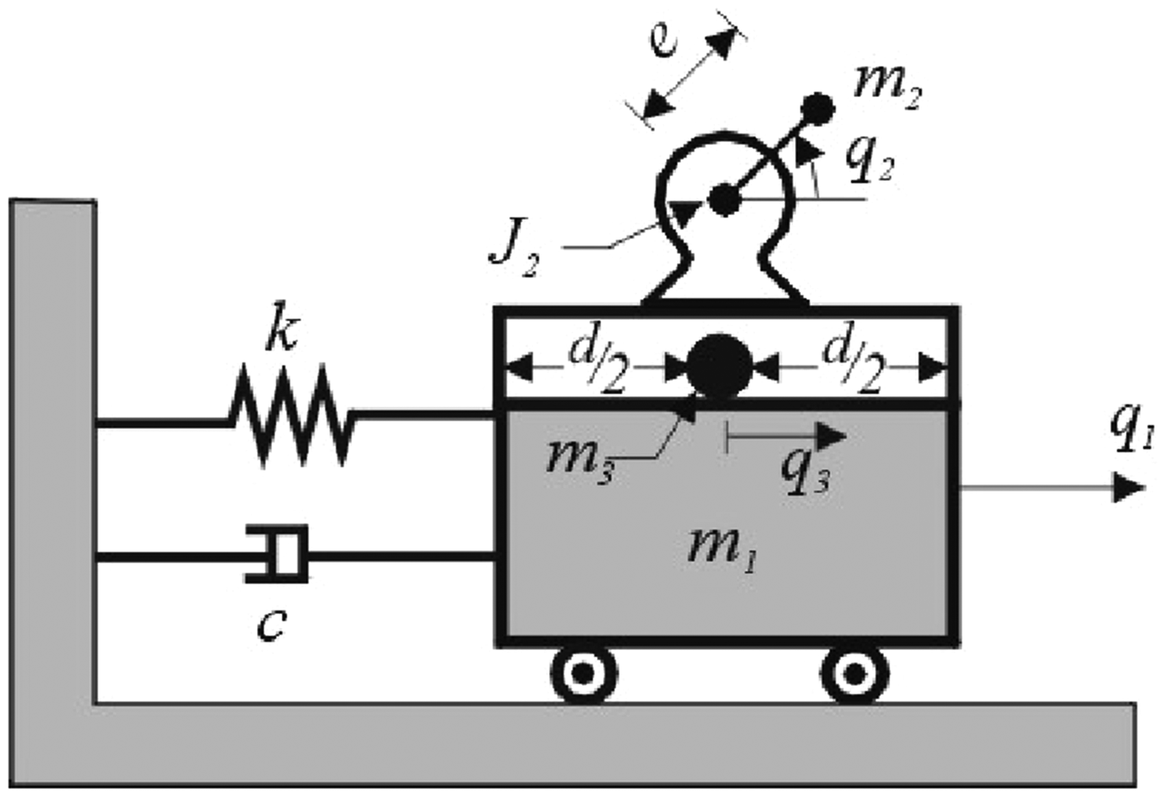
Vibro-impact systems have oscillating parts colliding against other vibrating components or limiting walls. An impact damper (ID) is one such vibro-impact system of practical importance. In this case, the vibration of the primary system is controlled by the momentum transferred during collisions with the secondary system, a free mass that displaces back and forth shocking against the walls of a carved box.^1,2 An example of a structural system with an ID is the motor foundation structure shown in Figure 1. In that figure, one can observe that the primary system is composed of two columns, a rigid beam and a motor installed on it. The columns present stiffness k and height h, the rigid beam has mass m₁. Generalized coordinate q₁ is related to the horizontal displacement of the mass fixed to the top of the columns. The motor has a rotating mass m₂ with eccentricity e and polar moment of inertia J₂. The angular displacement of m₂ is given by the generalized coordinate q₂. The secondary system is given by the free mass m₃, which displaces back and forth inside the carved box shocking against its walls. The carved box has length d and the position of this mass is given by generalized coordinate q₃. If the free mass exchanges kinetic energy with the primary system, it can reduce drastically the displacements of the motor foundation structure, acting as an ID.

Figure 1.

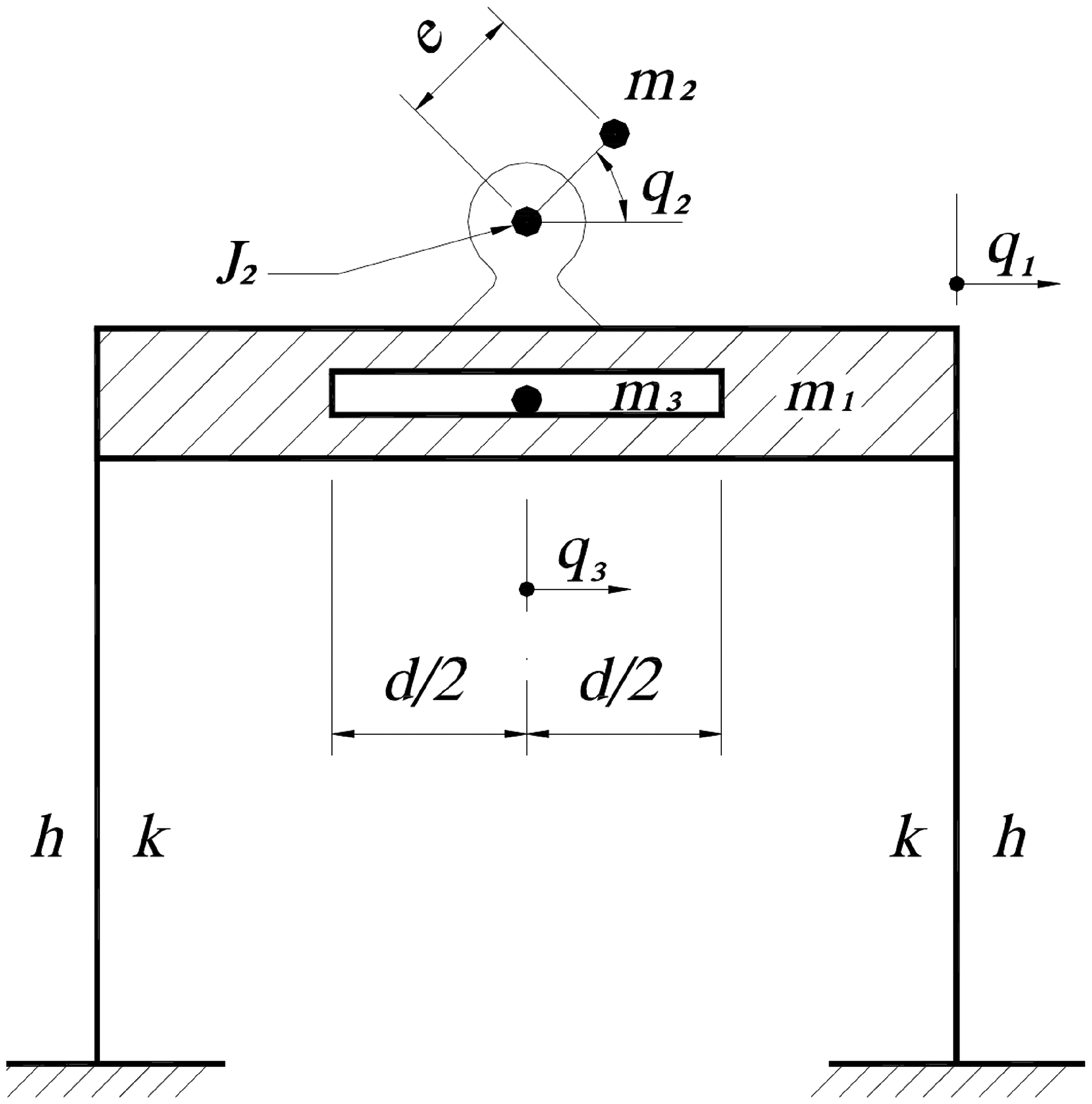
Model of a motor foundation structure.

The ideal power supply model supposes a periodic forcing function due to an external source, which is not perturbed by the motion of the structure. However, in practical situations, the dynamics of the forcing system cannot be considered as given a priori, and it must be taken as also a consequence of the dynamics of the whole system.^3,4 If the forcing system has a limited energy source, as that provided by an electric motor, for example, its own dynamics is influenced by that of the oscillating system that is being forced. This increases the number of degrees of freedom of the system and is called a non-ideal problem. In this paper, the system shown in Figure 1 is considered a non-ideal system, since the degree of freedom of the angular displacement of the motor q₂ is influenced by the structure displacement q₁.

The first mention of a non-ideal problem presented in the literature is the well-known Sommerfeld effect, named after the first researcher to observe it in 1902. Mikhlin et al.⁵ describe it as a phenomenon in which a large part of the vibration energy is transferred from the energy source straight to the resonance vibrations. In other words, in these problems the oscillating system interacts with the source of excitation. The Sommerfeld effect leads to large synchronous whirl amplitudes with considerable duration during passage through resonance. This occurs due to the coupling of vibration modes. Mathematically, the obtained nonlinear equations demonstrate that the system and its source are dynamically coupled and, consequently, they mutually interact.⁶ For simulating this phenomenon from a mathematic point of view, Dimentberg et al.⁷ performed a numerical study of coupled vibration and rotation of an unbalanced shaft with elastic suspension. Specifically, they investigated the passage through resonance with a limited power supply for the shaft rotation, by numerical integration of the nonlinear equations of motion. The results obtained out of a parametric study indicate strong influence of the damping ratio and a nondimensional unbalance parameter on the passage/capture threshold. The damping influence associated to a gyroscopic movement was studied by Samantaray.^8,9 Additionally, one year later, Samantaray et al.¹⁰ studied the direct or external damping and the rotating internal damping and showed this significant influence on the dynamic behavior of non-ideal systems when it is in the steady state behavior.

The Sommerfeld effect was largely studied by Konenko¹¹ in a classic book basically dedicated to non-ideal power sources. In that work, a cantilever beam, clamped in one extremity with a motor installed on its free extremity, was analyzed experimentally with the objective of detecting the interaction between the motor and the beam. The system presented unstable motions near resonance and the experiment could not reproduce the resonance curve of the equivalent ideal system. Starting from those results, researchers who considered non-ideal sources of energy in their models, for certain parameters, could also not reproduce the resonance curves, like those observed for ideal models, without discontinuities. It was not possible to find stable solutions in the resonance region, leading to jumps of motor frequencies and the structure displacements. Bharti et al.¹² examined a motor supported by flexible anisotropic supports/bearings. They concluded that due to the anisotropy in the supports, both forward and backward whirl motions of the rotor become excited, what causes a multi-Sommerfeld effect, in which two nonlinear jump phenomena are manifested at the first forward and backward critical speeds during rotor coast up and coast down. In the same direction, Quinn¹³ studied the influence of an anisotropic stiffness, due to the shaft cracks, in the response of a nonlinear, damped Jeffcott rotor. He realized that the anisotropy in the stiffness, in general, increases the values of the external torque over which a sustained resonant response can exist.

Investigation considering the modeling of a motor in a finite element model was performed by Karthikeyan et al.¹⁴ in order to study the Sommerfeld effect. They analyzed the increase in drive power input near resonance due to the fact that it contributes to increasing the transverse vibrations not producing increasing of the rotor spin. They generated a rotor response with a finite element model by assuming an ideal drive, and then the rotor system’s response with ideal drive was used in a power balance equation to theoretically predict the amplitude and speed characteristics of the same rotor system when it is driven by a non-ideal drive. Reviews of vibration problems that include resonance aspects affecting motors and their bases, including the Sommerfeld effect, have been presented by Balthazar et al.,¹⁵ Rocha et al.,¹⁶ and Varanis et al.¹⁷

Analyzing the region before resonance in a graph of motor frequency versus structure displacement (Figure 2), one notes that when the power given by the source to the motor is increased, the motor frequency is also increased. It is important to clarify here that each point in Figure 2 is related to steady state motions at a fixed given power level. However, as the motor frequency approaches the resonance region, the power source must supply more energy to increase the motor rotation, as part of this energy is being consumed by vibratory motions of the structure. A large change of power supplied to the motor results in just small changes in its frequency and a large increase of the structure displacements.

Figure 2.

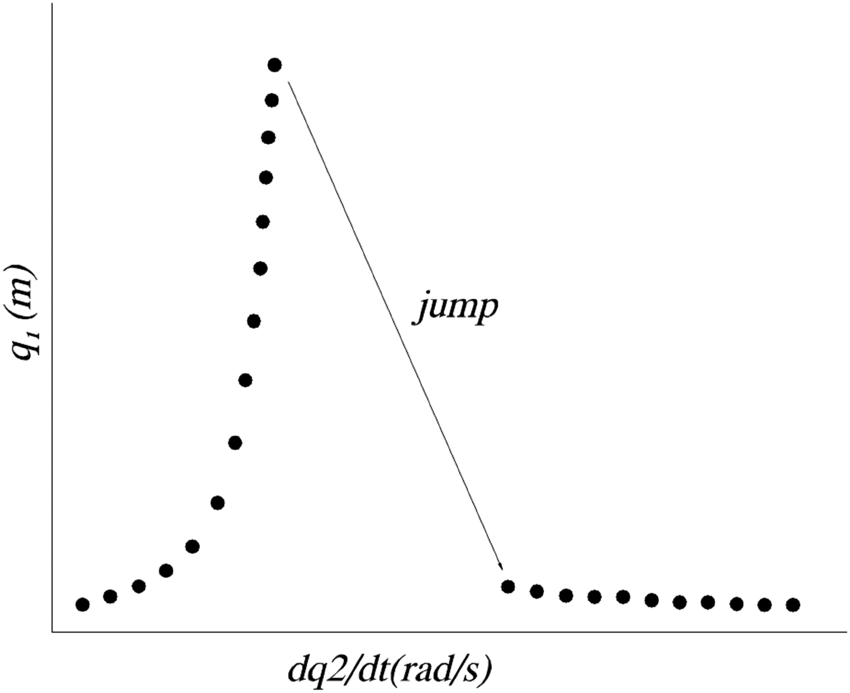
Displacement of the structure as a function of the frequency of the motor, as the motor energy is increased.

So, near to the resonance region, one can note that the additional power given to the motor only increases the structure displacement having little effect on the motor frequency. Right after the resonance, the structure displacement decreases drastically, as well as the motor frequency increases dramatically, a “jump” in the resonance curve. The increase of power required and the “jump” near the resonance region are called the Sommerfeld effect. Figure 3 shows what happens with the structure energy as the motor energy is increased in a non-ideal system.

Figure 3.

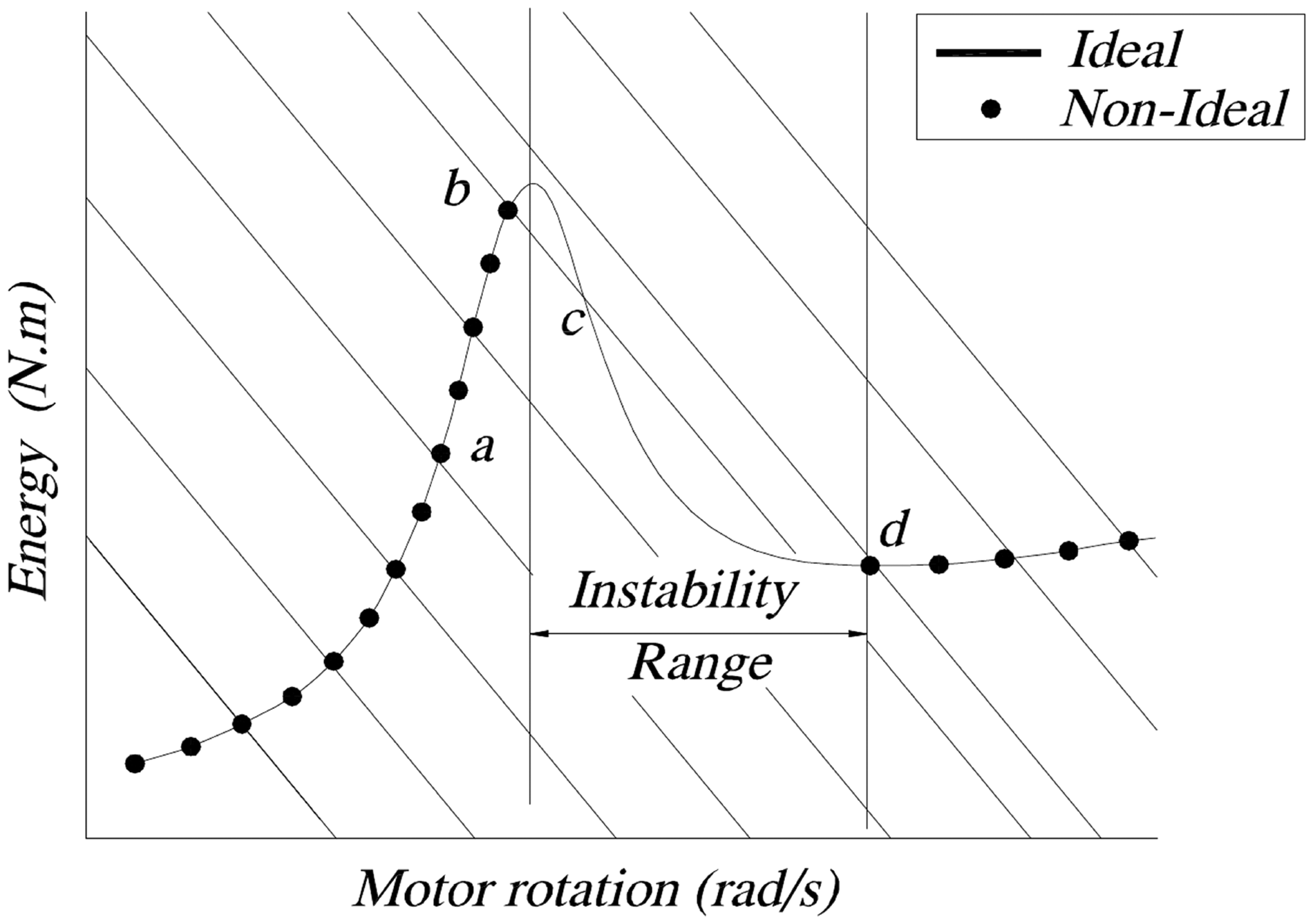
Energy of the structure as a function of the frequency of the motor, as the motor energy is increased.

As stated before, an unbalanced non-ideal DC motor foundation structure that suffers the Sommerfeld effect uses the energy supplied to the motor, before the resonance region, to increase the motions of the supporting structure. An efficient impact damping may tone down or even suppress that undesired phenomena without dissipation of energy.

The main goal of this paper is to formulate and solve optimization problems where the objective is to minimize the structure displacements in the stationary regime, properly designing the carved gap and the free mass.

IDs

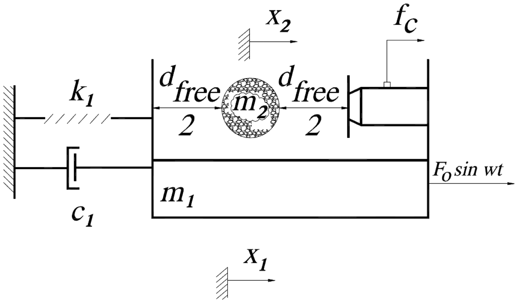
There are various types of IDs, starting with a single degree of freedom one. The simplest ID is called single particle impact damper (SPID) or single unit impact damper. In an ID there is only one free mass that shocks against the walls of a box. Popplewell et al.¹⁸ and Bapat et al.¹⁹ studied theoretically and experimentally the stable periodic vibrations of a SPID excited by a sinusoidal load, finding a reasonable correlation between theory and practice. A reproduction of the model proposed by those authors is shown in Figure 4.

Figure 4.

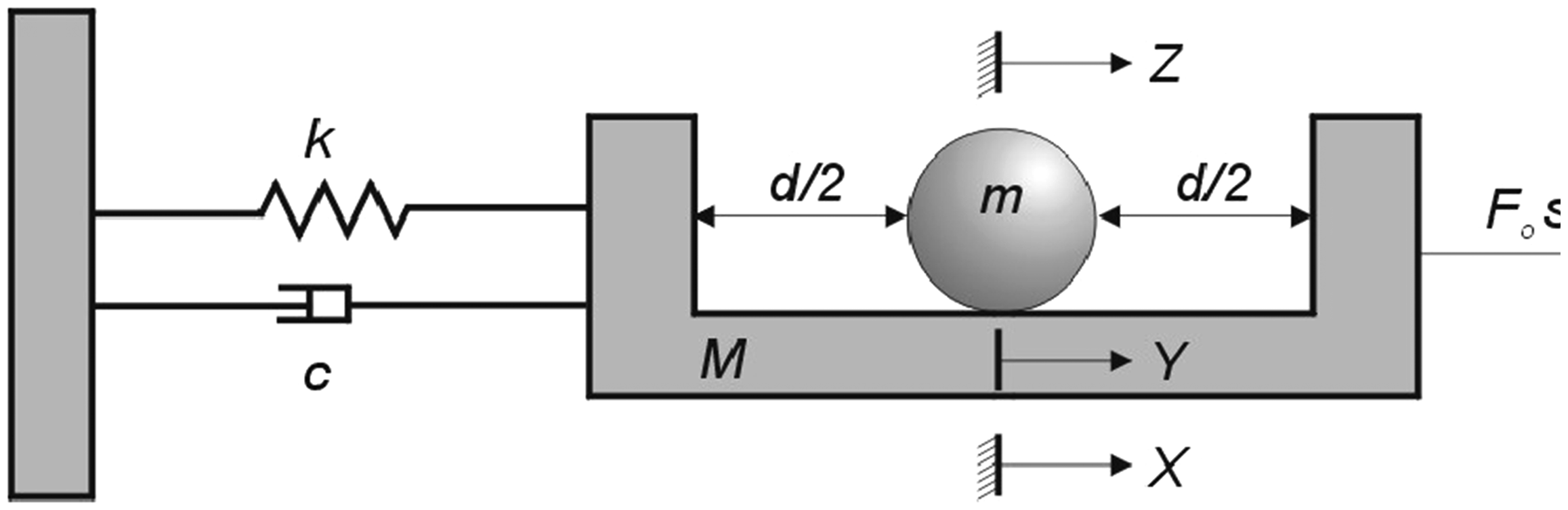
Model of SPID proposed by Popplewell et al.¹⁸

More recently, Duncan et al.²⁰ accomplished a numerical investigation of the performance of the damping of one SPID of vertical vibrations (Figure 5) for a vast interval of frequencies, amplitudes of vibrations, damping rates, and other parameters.

Figure 5.

Model of SPID studied by Duncan et al.²⁰

According to Bapat and Sankar,²¹ later confirmed by Popplewell and Liao,²² the efficiency of an ID decreases with the increase of the damping rate of a given structure, and it reaches the maximum when the rate between the frequency of loading and the natural frequency of vibration of the structure approaches unity, that is in resonance. Popplewell and Liao²² gave some expressions to compute the optimum gap d for a SPID design. There are several definitions of how to compute the efficiency of an ID, such as the rate between the maximum displacements computed with and without the ID, the rate between the maximum dynamic displacement and the static displacement, etc. In the present work, the authors consider the first definition given above to evaluate efficiency of the ID.

Starting from the basic idea of the SPID, researchers developed others variation of ID, such as the multi-particle impact damper (MPID), shown in Figure 6. This ID contains a large quantity of particles, producing dissipation of energy also through the friction between the particles. Several authors have studied the behavior of the MPID, among them Saeki²³ and Marhadi and Kinra.²⁴ The studies conducted by those authors analyzed the influence of the size of the box, the kind of granular material of particles, and the specific mass in the performance of the ID.

Figure 6.

Model of MPID proposed by Saeki.²³

Now, the bean bag impact damper (BBID) is described, name given because of the similarity with a bean bag, which consists of several particles confined inside a plastic bag. According to Popplewell and Semercigil,²⁵ who investigated the performance of the BBID shown in Figure 7, it has the advantage of minimizing the noise due to the fact that the bag has a certain flexibility of shape and increases damping due to the interaction between the particles.

Figure 7.

Model of BBID.

Note that all ID models shown present an external ideal load given by a sinusoidal function, which is not influenced by the structure displacement. Here it is considered a non-ideal power source model, in which the interaction between the loading and the vibrating system is taken in consideration. The non-ideal system is obtained replacing the sinusoidal external loading by a rotor attached to the structure driven by a motor. The mathematical model of a non-ideal system with an ID, developed by Feitosa,²⁶ is shown in Figure 8. This work with another of same research group^27,28 could be considered as the benchmark for this problem. Further, in the present work, the results from Brasil et al.²⁸ and those obtained here will be compared, but they just analyzed the system and the reduction of vibration that the design could provide to the structural system. In the present work, the idea is to optimize the mass and the gap to minimize the vibrations of the main structure.

Figure 8.

Non-ideal model with ID.²⁶

The equations of motion

In this section, the equations of motion for the system given by Figures 1 and 8 are derived. First, the equations of motion are written for the non-controlled (NC) model, using the Lagrange’s equations. A Rayleigh’s dissipation function to model the viscous structural damping is considered, as well as to model the mechanisms of supplying and dissipating of energy in the motor, the latter due to internal friction, as

ℑ = \frac{1}{2} (c {\dot{q}}_{1}^{2} + b {\dot{q}}_{2}^{2}) - a {\dot{q}}_{2}

(1)where c is the constant of the viscous structural damping, while a and b are motor constants possibly given by the manufacturer.

Introducing the total potential energy, the kinetic energy, and the dissipation function into Lagrange’s equations, the following pair of nonlinear ordinary differential equations of motion for the NC model is obtained

M {\ddot{q}}_{1} + c {\dot{q}}_{1} + k q_{1} = S ({\ddot{q}}_{2} \sin q_{2} + {\dot{q}}_{2}^{2} \cos q_{2})

(2)

J {\ddot{q}}_{2} + b {\dot{q}}_{2} - a = S ({\ddot{q}}_{1} \sin q_{2} - g \cos q_{2})

(3)where

M = m_{1} + m_{2}

S = m_{2} e

, and

J = J_{2} + m_{2} e^{2}

Next, the impact control by means of the third free mass m₃ is introduced. This mass is free to displace back and forth inside the carved box, fixed to the structure. This leads to an additional degree of freedom. The displacement of this point mass is denoted q₃, which is bounded by the moving walls of the carved gap. The additional equation of motion for this coordinate, assuming that there is no friction between the mass and the box surface, is the uncoupled second-order homogeneous differential equation

{\ddot{q}}_{3} = 0

(4)

| q_{3} - q_{1} | \geq d / 2

(5)it means mathematically that the impact already happened. Thus, it is necessary to compute the initial velocities

{\dot{q}}_{1 a}

and

{\dot{q}}_{3 a}

, at the time t_a, immediately after each impact between the mass m₃ and the main structure of mass m₁. To calculate

{\dot{q}}_{1 a}

and

{\dot{q}}_{3 a}

{\dot{q}}_{3 a}

, inelastic collisions are assumed with restitution coefficient 0 < r < 1. This quantity is defined as the ratio between the differences of velocities of the masses when they approach each other, just before the collision, and the same difference when they separate one from other, just after the impact. So, r is computed as

r = - \frac{{\dot{q}}_{1 a} - {\dot{q}}_{3 a}}{{\dot{q}}_{1 b} - {\dot{q}}_{3 b}} = \frac{- (velocity o f separation)}{(velocity o f approach)}

(6)

As there are two unknown velocities after impact to determine, another equation is needed besides equation (6). That will be the statement of the conservation of the linear momentum

m_{1} {\dot{q}}_{1 a} + m_{3} {\dot{q}}_{3 a} = m_{1} {\dot{q}}_{1 b} + m_{3} {\dot{q}}_{3 b}

(7)

Solving equations (6) and (7), the initial velocities are obtained, just after the impact, to allow integration of equations (2) to (4)

\begin{matrix} {\dot{q}}_{1 a} = \frac{(m_{1} - r m_{3}) {\dot{q}}_{1 b} + m_{3} (1 + r) {\dot{q}}_{3 b}}{m_{1} + m_{3}}, {\dot{q}}_{3 a} = \frac{(m_{3} - r m_{1}) {\dot{q}}_{3 b} + m_{1} (1 + r) {\dot{q}}_{1 b}}{m_{1} + m_{3}} \end{matrix}

(8)

For a given time t after a certain impact and before the following one, velocities and displacements by simple integration of the single equation (4) are determined.

The augmented Lagrangian method

To solve the structural optimization problems formulated in this paper, it is necessary to adopt an optimization algorithm capable of dealing with static and dynamic constraints, as well as nonlinear functions. A nonlinear optimization problem with static and dynamic constraints is presented as follows: find the design variables x ∈ $R^{n}$ that minimize the nonlinear objective function f( x ) subjected to the nonlinear constraint functions

Static

g_{i} (x) = 0;   i= 1,l

(9)

g_{i} (x) \leq 0;   i=l+ 1,m

(10)and dynamic, ∀ t ∈ [t₀,t_f]

g_{i} (x, t) = g_{i} (x, z (t), \dot{z} (t), \ddot{z} (t), t) = 0; i=m+ 1,l′

(11)

g_{i} (x,t) = g_{i} (x, z (t), \dot{z} (t), \ddot{z} (t),t) \leq 0; i=l′ 1,m′

(12)

In dynamics of structures, the displacement vector z (t) must satisfy the equations of motion, a system of second-order ordinary differential equations

\begin{matrix} M (x, \ddot{z}, \dot{z}, z, t) \ddot{z} (t) + C (x, \ddot{z}, \dot{z}, z, t) \dot{z} (t) \\ + R (x, \ddot{z}, \dot{z}, z, t) = p (x, \ddot{z}, \dot{z}, z, t) \end{matrix}

(13)

The initial conditions are $\dot{z} (t_{0}) = {\dot{z}}_{0} and z (t_{0}) = z_{0}$ , where M $(x, \ddot{z}, \dot{z}, z, t)$ and C $(x, \ddot{z}, \dot{z}, z, t)$ are, respectively, the mass and damping matrix, the vector R $(x, \ddot{z}, \dot{z}, z, t)$ is the generalized elastic force, and p $(x, \ddot{z}, \dot{z}, z, t)$ is the generalized force vector. Equations (9) and (10) include, for example, limits of the design variables. Equations (11) and (12) represent constraints with dynamic responses such as the maximum and minimum values of the displacements z (t), dynamic strain and stress. The initial and final times are t₀ and t_f, respectively.

During the designing process, a set of parameters, denoted design variables x , are selected to define the system that will be designed. Once the design variables are specified, the vector z (t) is determined by equation (13). The displacements are called state variables, as they determine the structure configuration for every t ∈ [t₀,t_f], and equation (13) is the state equation. The constraints with dynamic responses are explicit functions of state variables and implicit functions of the design variables. Usually, in structural optimization problems with dynamic constraints, the state variables vector is denoted as z (t). As one can note, in this work the notation q (t) for the displacement vector is also used.

There are several methods to solve the problem defined by equations (9) to (13). The augmented Lagrangian method is used here. The Lagrangian functional is created using the objective and the constraint functions, associated to the Lagrange multipliers and penalty parameters

Φ (x, u, r) = f (x) + P (g (x), u, r)

(14)

P( g ( x ), u , r ) is a penalty functional, $u \in R^{m'}$ and $r \in R^{m'}$ are, respectively, the Lagrange multipliers and the penalty parameters. It is possible to determine u * and r * so that the minimum point x * of the functional defined in equation (14) is the minimum point of the problem defined by equations (9) to (13). As iterative methods are used to find u * and r *, it is necessary to adopt a stopping criterion.

The augmented Lagrangian method defines procedures for updating penalty parameters and Lagrange multipliers. This method can be simply described by the algorithm:

Step 1. set k = 0, estimate vector u and r ;

Step 2. minimize Φ( x , u ^k , r ^k ) with respect to x . Let x ^k be the best point obtained in this step;

Step 3. if the stopping criterion is satisfied, stop the iterative process;

Step 4. update u ^k , and r ^k , if necessary;

Step 5. set k = k + 1 and go to step 2.

The multipliers method is simple, and its essence is contained in steps 2 and 4. The functional (14) can be defined in several ways.

In the present work, the Lagrangian functional adopted to solve the problem with dynamic response, defined by equations (9) to (13), is defined by

\begin{array}{l} Φ (x, θ, r) = f (x) + \frac{1}{2} {\sum_{i = 1}^{l} r_{i} {(g_{i} (x) + θ_{i})}^{2} + \sum_{i = l + 1}^{m} r_{i} {(g_{i} (x) + θ_{i})}_{+}^{2}} \\ + \frac{1}{2} \int_{t_{0}}^{t_{f}} {\sum_{i = m + 1}^{l'} r_{i} {(g_{i} (x, t) + θ_{i})}^{2} + \sum_{i = l' + 1}^{m'} r_{i} {(g_{i} (x, t) + θ_{i})}_{+}^{2}} d t \end{array}

(15)

In equation (15) r_i are the penalty parameters and θ_i define the Lagrangian multipliers as u_i = r_iθ_i, for i = 1,…,m′. Note that, in equation (15), the dynamic constraint functions are integrated at the time interval and combined with the objective function to obtain the Lagrangian functional. At steps 2 and 3, it is necessary to adopt a stopping criterion. Here, it is considered the following criterion

k < p

(16)where p is the maximum number of iterations, and

‖ \nabla Φ (x^{k}, u^{k}, r) ‖ \leq ε and

(17)

\begin{array}{l} K_{b} = \max {\max_{1 \leq i \leq l} | g_{i} (x^{(k)}) |; \max_{l + 1 \leq i \leq m} \\ |max(g_{i} (x^{(k)}), - θ_{i})|; \\ \max_{1 \leq i \leq l′} (\max_{t_{0} \leq t \leq t_{f}} | g_{i} (x^{(k)},t)|); \\ \max_{l' + 1 \leq i \leq m′} (\max_{t_{0} \leq t \leq t_{f}} |max(g_{i} (x^{(k)},t), - θ_{i} (t)) |)} \leq ε \end{array}

(18)

In equation (18) K_b is the maximum constraint violation and in equations (17) and (18) ε is the tolerance. If the algorithm is not converging, condition (16) states a finite number of iterations. Arora et al.²⁹ noted, in several analyzed examples, that the best value for p is 2n. The process of updating the Lagrange multipliers and penalty parameters and more details on the adopted algorithm are to be found in Arora et al.²⁹ and Chahande and Arora.³⁰

A computation program was developed by the authors, based on this augmented Lagrangian method. The following numerical algorithms were utilized to implement this method:

to solve the equations of motion (12), Newmark’s (NW) method or fifth-order Runge–Kutta’s (RK) method is used;

related to unconstrained minimization (step 2), it used conjugated gradient method with Armijo line search;

to calculate the gradient vector, the finite difference method is used;

to integrate equation (14), Simpson’s rule is used;

to solve linear systems, Cholesky decomposition is used.

Originally, the standard NW’s method was developed for linear equations. However, in the present work, the equations of motion are nonlinear equations. So, a NW’s method was developed conjugated with the Newton–Raphson’s method. Instead of obtaining a linear equation to be solved in each time step, as in classical NW’s method, a nonlinear equation is solved by Newton–Raphson’s method. In the “Numerical results and comments” section, the performance of this NW’s method compared with the performance of the fifth-order RK’s method will be discussed.

The optimization problems

Consider the elevated machine foundation shown in Figure 1. The objective is to design a carved box and a free mass that minimize the maximum structure displacement in the steady state regime. In other words, minimize the maximum displacement of the degree of freedom q₁, properly varying the parameters d and m₃. Thus, the natural design variables of this problem are the carved gap width d, considered here as the design variable x₁, and the mass m₃, considered as design variable x₂. Since q₁ is a state variable, it cannot be directly the objective function because the objective function is a function of the design variables. To minimize q₁ an artificial design variable x₃ was created, which is the maximum value allowable to q₁ and also the objective function. The design variable vector is x ^T = {x₁ x₂ x₃} ≡ {d m₃ max(q₁)}.

The optimization problem is to determine x ∈ ℜ³ that minimizes the objective function

f (x) = x_{3}

(19)subjected to the static constraints

{d \geq 0} \equiv {g_{1} (x) = - x_{1}}

(20)

{m_{3} \geq 0} \equiv {g_{2} (x) = - x_{2}}

(21)subjected to the dynamic constraint

{q_{1} \leq x_{3}} \equiv {g_{3} (x, t) = q_{1} - x_{3}, \forall t \in [t_{0}, t_{f}]}

(22)

The state variables must satisfy the state equations, given by equations (2) to (4) and (8). It is important to remember that the motor constant a assumes several values in a given interval [a₀,a_f], according to the power supplied to the motor and the discretization adopted to the interval. For each value of a there is one solution for the equations of motion.

As stated, the objective is to minimize q₁ in the stationary regime. So, when x₃ is minimized, q₁ is also minimized in both transient and stationary regime. Here, emphasis is given to the steady state regime. Therefore, it is defined now q_s₁, ∀ t ∈ [t_s,t_f], that is the displacement q₁ in the stationary regime, and t_s is the time when the stationary regime starts. Searching the best formulation for the problem of minimizing the displacement q_s₁, other objective functions were defined as follows

f (x) = \max_{a_{0} \leq a \leq a_{f}} \max_{t \in [t_{s}, t_{f}]} | q_{s 1} |

(23)

f (x) = \sum_{a = a_{0}}^{a_{f}} \max_{t \in [t_{s}, t_{f}]} | q_{s 1} |

(24)

f (x) = \frac{1}{2} \sum_{a = a_{0}}^{a_{f}} \max_{t \in [t_{s}, t_{f}]} {| q_{s 1} |}^{2}

(25)

f (x) = 2 \sum_{a = a_{0}}^{a_{f}} \max_{t \in [t_{s}, t_{f}]} {| q_{s 1} |}^{0.5}

(26)

When equation (23) is taken as the objective function, the constraint function, given by equation (22), must be computed ∀ t ∈ [t_s,t_f]. In case of using one of the objective functions given by equations (24) to (26), the constraint (22) is suppressed, and the design variable vector becomes x ∈ ℜ², such as x ^T = {x₁ x₂} ≡ {d m₃}.

There are several methods to solve the problems defined by equations (19) to (26), such as the sequential quadratic programing and the augmented Lagrangian method. As stated, in this work the augmented Lagrangian method is used as described in the “The augmented Lagrangian method” section.

Numerical results and comments

The following numerical values for the structural parameters were adopted: k = 49152 N/m and M = 2 kg, leading to natural frequency ω = 156.767 rad/s; S = 0.001 kg m; J = 1.776 × 10⁻⁴kg m²; c = 3.1353 N s/m, equivalent to 0.5% of the critical damping. In equation (8) m₁ = M is adopted. The motor parameters are a, increasing from a₀ = 0.25 up to a_f = 0.50, with step of 0.01, and b = 0.002 N m s. For the dynamic analysis, the initial values for the state variables are

q^{T} (0) = {\begin{cases} 0 & 0 & d / 2 \end{cases}} and {\dot{q}}^{T} (0) = {\begin{cases} 0 & 0 & 0 \end{cases}}

(27)and the time interval is t ∈ [0,10] s, discretized into 4801 equally spaced grid points. As stated, the values of d and m₃ will be computed by solving the optimizations problems already defined.

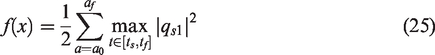
The first analysis addresses the issue of what time integration method, NW or fifth-order RK is more precise and stable for the proposed problems. So, the NC problem was solved, considering only the degrees of freedom q₁ and q₂, and the results plotted in Figure 9.

Figure 9.

Comparison between NW and fifth-order RK’s methods for NC problem. NW: Newmark; RK: Runge–Kutta.

One can see in this figure that the precision of both methods is basically the same, but it was noted, based on others results of this research, that NW is more stable, specifically near to the resonance region. It is important to clarify here that each point in this graph is related to steady state motions at a given value of a, and it means a certain amount of power supplied to the motor. One can note that there are 26 grid points in the graph, which is the discretization presented above for the values of a. As the value of a is increased, points are generated from left to right in the figure. So, left points are related to lower levels of power. Based on the results of Figure 9 and the considerations presented above, NW’s method was chosen to solve the equations of motion in the following simulations. Curves shown in Figure 9 are also called resonance curves.

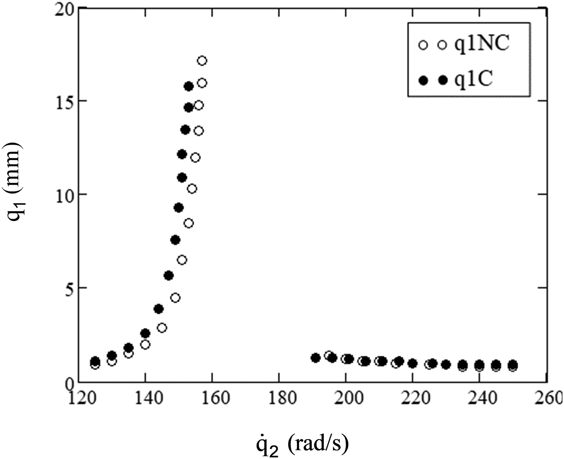
It is important to observe that the problem of controlling the vibrations is very sensitive to chosen values of d and m₃. If the choice of these values is not adequate, just small differences will be observed in the resonance curve, as can be noted in Figure 10, when values of d = 2.0 cm and m₃ = 0.010 kg were chosen.

Figure 10.

Resonance curve for NC and controlled (C) systems for d = 2.0 cm and m₃ = 0.010 kg. NC: non-controlled.

Analyzing Figure 10, it can be noted that for a = 0.38 the largest value of structure displacement is around 17 mm. So, in the first attempt to optimize the carved box, it was fixed the value of a equal to 0.38 and solved the optimization problem described by equations (19) to (22), trying to minimize the structure displacement in this region. As the augmented Lagrangian method is iterative, it is necessary to choose an initial design. In the problem the initial design {2.0 cm; 0.01 kg; 17 mm} was adopted (Figure 10). The optimum values of the design variables obtained in this case, with eight iterations, were d = 0.1 cm, m₃ = 0.111 kg. For a = 0.38, the value fixed in this case, a very low value of displacement was obtained, around 1 mm—a significant reduction when it is compared with the previous value of 17 mm. But when all the resonance curve is plotted, one can note that for values of a lower than 0.38 the displacements were very large, reaching max(q₁) = 16 mm when a = 0.37, as it is shown in Figure 11. Thus, these results were good for a = 0.38, but not for other values of a. Regarding this solution, one advantage is that larger values of motor rotation can be reached with a smaller power. The jump on the resonance region happens with lower values of energy.

Figure 11.

Resonance curve for NC and C systems for d = 0.1 cm and m₃ = 0.111 kg. C: controlled; NC: non-controlled.

In the next trial to obtain an optimum design, starting from the initial design {1.5 cm; 0.183 kg; 14 mm}, the optimization problem described by equations (19) to (22) was solved for all values of a defined previously. With eight iterations, an optimum design with d = 2.8 cm, m₃ = 0.178 kg, and max(q₁) = 12 mm was obtained, as one can see in Figure 12. The reduction of the maximum displacement, before the resonance region, is of 31%. This is very significant. But after that, when the motor works with higher frequencies, it reached up to 212%. That is, the displacements more than triplicated. Usually, it is expected of a motor to give the maximum power allowable, so this solution may be practical for lower motor frequencies but not for higher frequencies.

Figure 12.

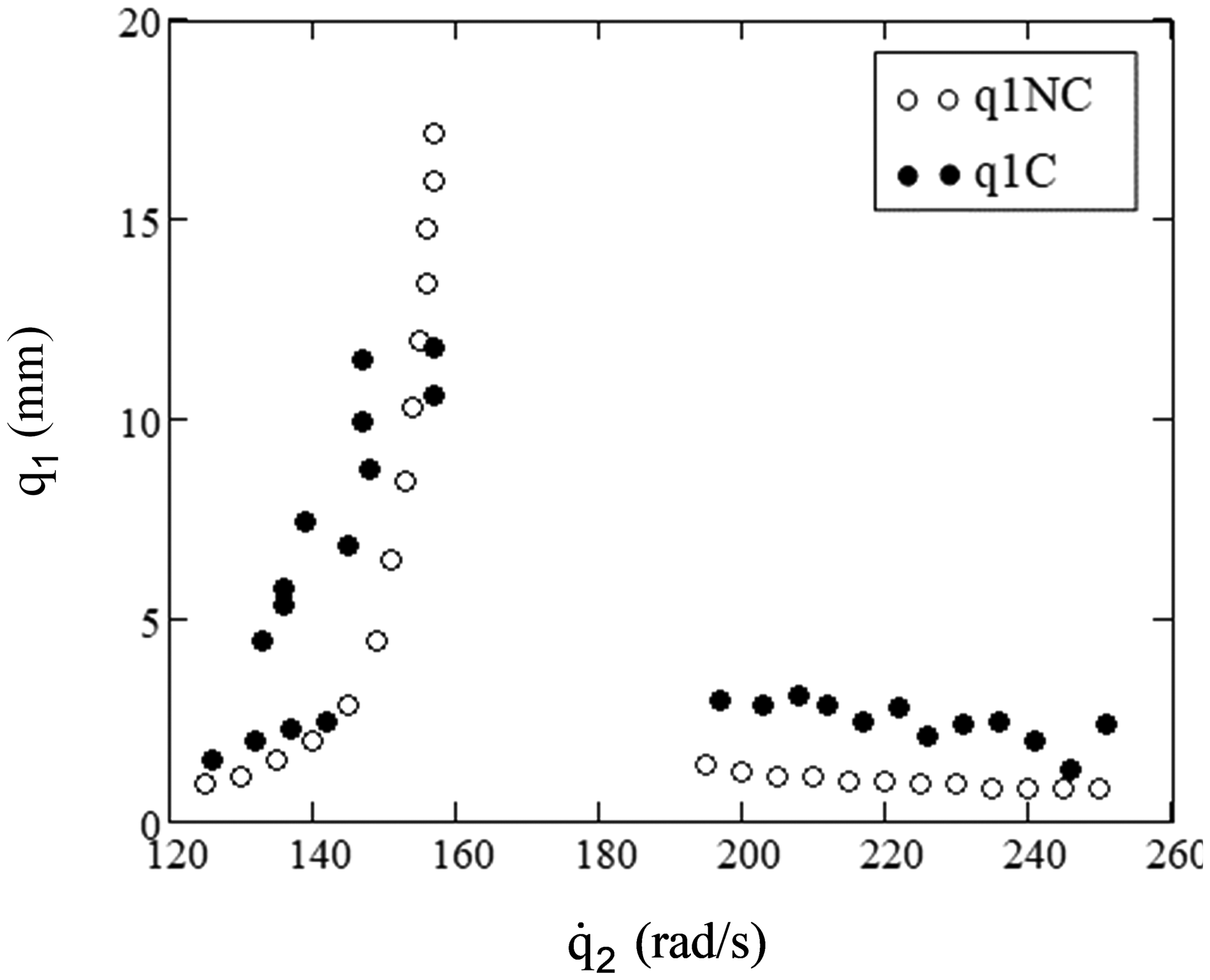
Resonance curve for NC and C systems for d = 2.8 cm and m₃ = 0.178 kg. C: controlled; NC: non-controlled.

Solving the same problem stated above but starting from the design {3.3 cm; 0.313 kg; 8 mm}, with eight iterations, an optimum design with d = 0.7 cm, m₃ = 3.881 kg, and max(q₁) = 5.8 mm was obtained, as shown in Figure 13.

Figure 13.

Resonance curve for NC and C systems for d = 0.7 cm and m₃ = 3.881 kg. C: controlled; NC: non-controlled.

What it is observed in this design is that it increases drastically the mass of the system, practically triplicating it, and reduces the carved gap to millimeters. The consequence is that the resonance region disappears, because the equivalent natural frequency of vibration of the system, with all this mass, reduces to around 90 rad/s, that is out of the plotting region. In practice, this is not viable because a very significant change in the mass of the system is necessary. Regarding the displacements, the design reduces the amplitudes in a part of the curve but increases drastically for higher frequencies, what is not reasonable, as stated previously. One can note that in all the problems solved until now, the augmented Lagrangian method program converged with eight iterations, which is the minimum number of iterations adopted in the implementation.

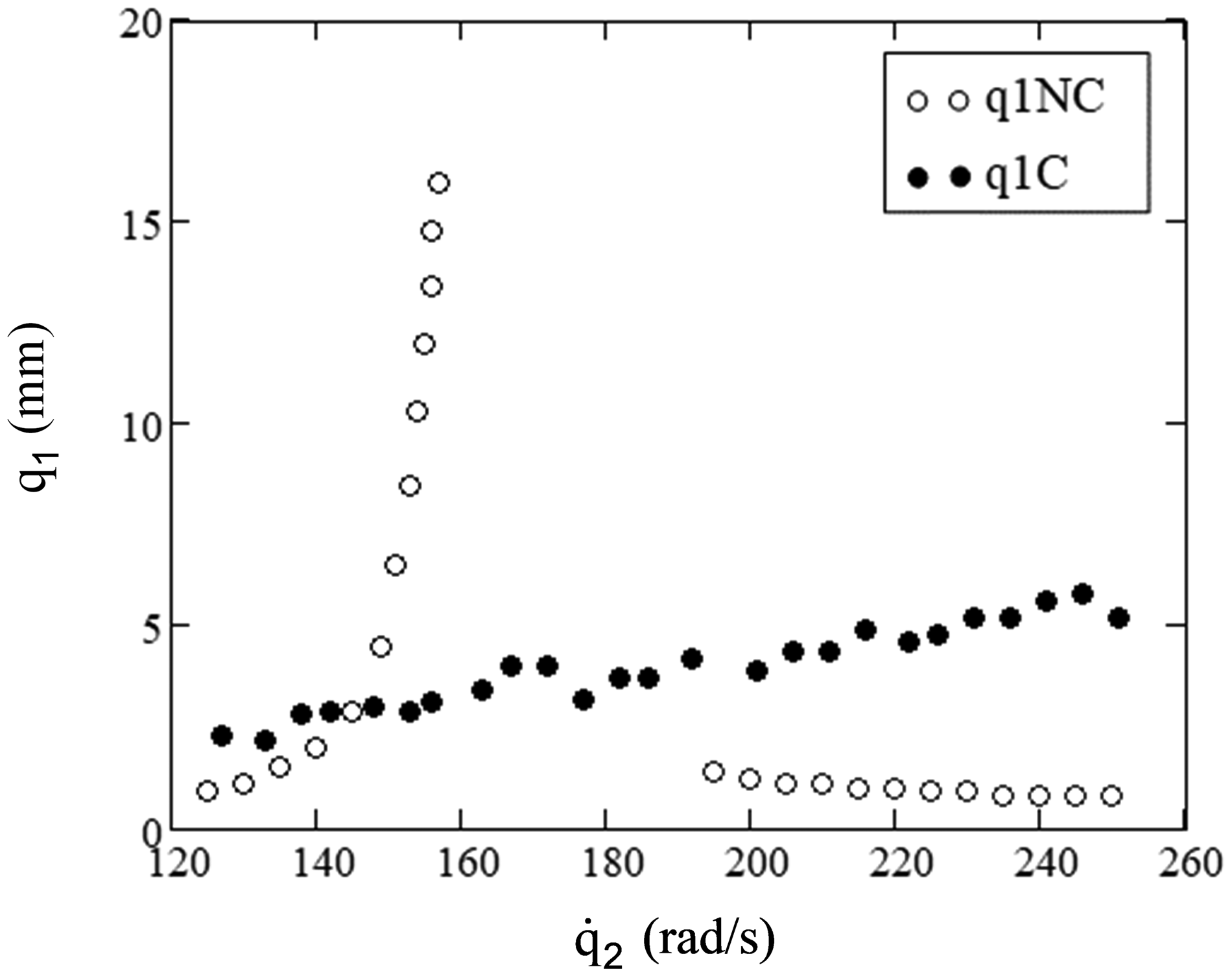
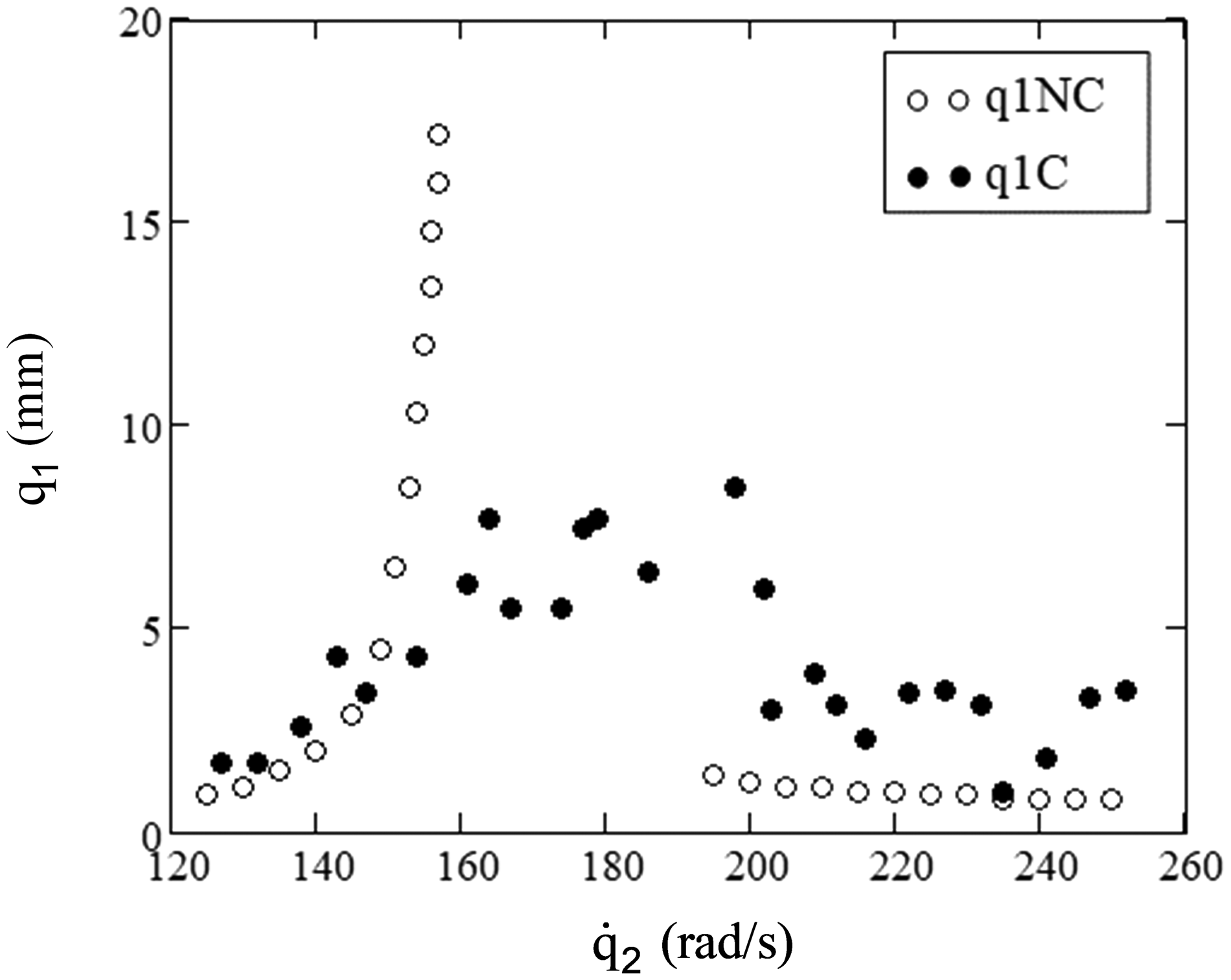
Now, trying to put more emphasis in the stationary regime, the solution of the optimization problem considering the objective function by equation (23) and constraints functions given by equations (20) to (22) will be presented. Adopting the initial design {6.0 cm; 0.200 kg; 8 mm}, with eight iterations, an optimum design with d = 3.3 cm, m₃ = 0.313 kg, and max(q₁) = 8.0 mm was obtained, as shown in Figure 14. One can note that this optimum design eliminates the resonance region and reduces the maximum displacement by 53% but increases the displacements for higher motor frequencies. The values obtained for m₃ and d are very reasonable, since they are easy to be implemented in practice and do not change significantly the mass of the system.

Figure 14.

Resonance curve for NC and C systems for d = 3.3 cm and m₃ = 0.313 kg. C: controlled; NC: non-controlled.

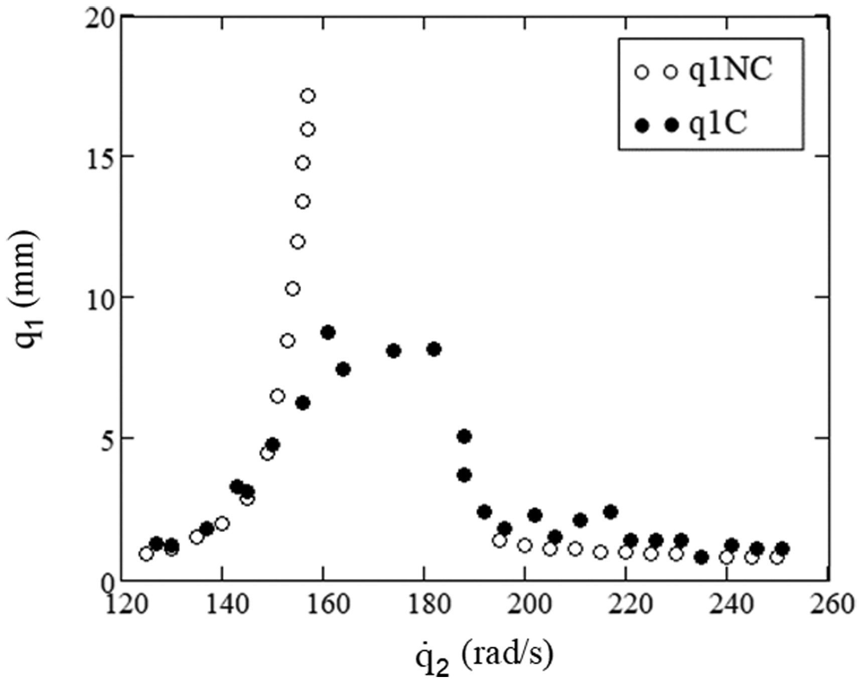
Continuing with the strategy of giving more emphasis in the stationary regime, the solution of the optimization problem given by the objective function, equation (24), and constraint functions given by equations (20) and (21) will be presented. Note that the number of design variables is now equal to 2 and there are only two constraints applied to the problem. The initial design {3.3 cm; 0.313 kg} was adopted, that is the optimum design of the problem described previously (Figure 14). Solving the problem, with eight iterations, the optimum design with d = 2.7 cm, m₃ = 0.339 kg was obtained. For this design the objective function, equation (24), is equal to 291. The maximum displacement, in the stationary regime, is 8.5 mm, as shown in Figure 15. This optimum design also eliminates the resonance region and reduces the maximum displacement by 50%, but increases the displacements for higher motor frequencies. The values obtained for m₃ and d are very reasonable in this case too, easy to be implemented in practice and do not change significantly the mass of the system.

Figure 15.

Resonance curve for NC and C systems for d = 2.7 cm and m₃ = 0.339 kg. C: controlled; NC: non-controlled.

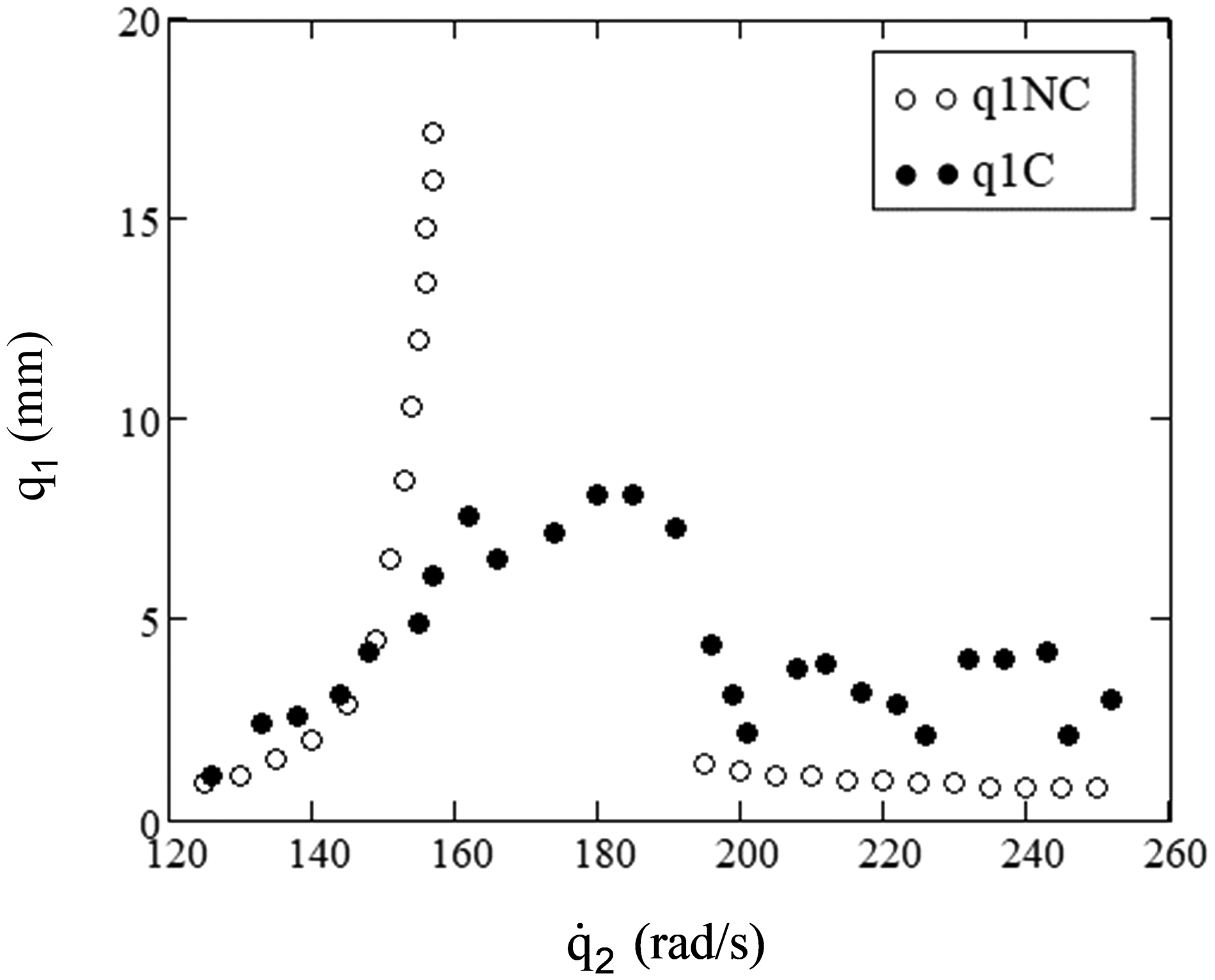
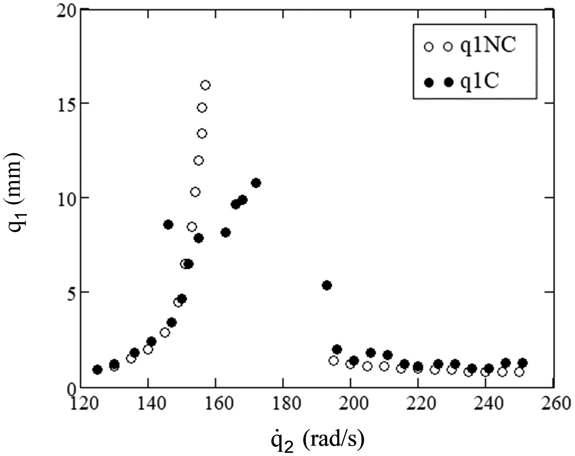
Next, the solution of the optimization problem given by the objective function, equation (25), and constraint functions given by equations (20) and (21) will be presented. Note again that in this problem the number of design variables is now equal to 2 and there are only two constraints applied on the problem. The initial design {2.7 cm; 0.339 kg} was adopted, that is the optimum design of the problem described previously (Figure 15). Solving the problem, with eight iterations, an optimum design with d = 7.4 cm, m₃ = 0.102 kg was obtained. For this design, the objective function, equation (25), is equal to 84. The maximum displacement, in the stationary regime, is 8.8 mm, as shown in Figure 16. This optimum design also eliminates the resonance region, reduces the maximum displacement by 48%, and does not increase significantly the displacements for higher motor frequencies. The values obtained for m₃ and d are very reasonable for practical purposes in this case too.

Figure 16.

Resonance curve for NC and C systems for d = 7.4 cm and m₃ = 0.102 kg. C: controlled; NC: non-controlled.

At this point, the solution of the optimization problem given by the objective function, equation (26), and constraint functions given by equations (20) and (21) will be presented. Note that in this problem the number of design variables is now equal to 2 and there are only two constraints applied on the problem. It was adopted the initial design {2.7 cm; 0.339 kg}, that is the design of Figure 15.

Solving the problem, with eight iterations, an optimum design with d = 10.5 cm, m₃ = 0.049 kg was obtained. For this design, the objective function, equation (26), is equal to 92. The maximum displacement, in the stationary regime, is 10.8 mm, as shown in Figure 17. This optimum design does not totally eliminate the resonance region, but it reduces the maximum displacement by 36% and does not increase significantly the displacements for higher motor frequencies. The values obtained for m₃ and d are very reasonable for practice in this case too.

Figure 17.

Resonance curve for NC and C systems for d = 10.5 cm and m₃ = 0.049 kg. C: controlled; NC: non-controlled.

In Figure 18 the results obtained here are compared with those given by the benchmark reference.²⁸ One can note in Figure 18(b) that the present solution eliminated the “jump” due to Sommerfeld effect and in Figure 18(c), for higher machine frequencies, the control on the amplitude of vibration is more effective in the present work. The solution for the NC problem is shown in Figure 18(a) and the numerical results practically match.

Figure 18.

Comparison of the present work and Brasil et al.²⁸: (a) NC (Figure 9 NW present work), (b) controlled Figure 16 present work, and (c) Figure 17 present work. C: controlled; NC: non-controlled.

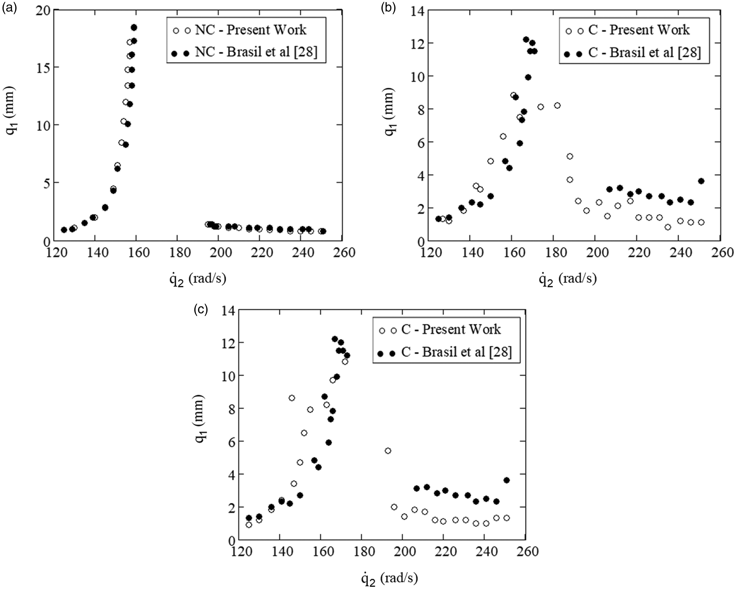
Table 1 summarizes the results obtained in all formulations proposed and solved in the present paper. From the results and comments presented, a conclusion is reached that the formulation considering the objective function by equation (25) was the one that eliminated the resonance region, reduced the maximum displacement by 48%, and did not substantially increase the displacements for higher values of motor frequency. In a general way, this formulation presented the best performance. However, if it is only considered the displacements for higher motor frequencies, the formulation presented by equation (26) gave the best results. If only the maximum structure displacement for the reasonable designs obtained is taken into consideration, formulation provided by equation (23) gave the best solution.

Table 1.

Summary of the designs obtained in this work.

Status	a	Objective	Optimum design
Status	a	Function	d (cm)	m₃ (kg)	Equation (23)	Equation (24)	Equation (25)	Equation (26)
NC-RK	0.25–0.50	–	–	–	17.8	791.3	135.8	101.3
NC-NW	0.25–0.50	–	–	–	17.2	682	123.4	96.2
C-RK	0.25–0.50	–	2	0.01	17.4	767.9	136.5	103
C-NW	0.25–0.50	–	2	0.01	16.9	662.5	123.8	97.6
C-NW	0.38	Equation (19)	0.1	0.11	15.8	567.6	114.1	93.8
C-NW	0.25–0.50	Equation (19)	2.8	0.178	11.8	421.7	121	106
C-NW	0.25–0.50	Equation (19)	0.7	3.881	5.8	221.8	104.2	103.3
C-NW	0.25–0.50	Equation (23)	3.3	0.313	8.1	294.1	112.1	105
C-NW	0.25–0.50	Equation (24)	2.7	0.339	8.5	291.4	110.8	104.1
C-NW	0.25–0.50	Equation (25)	7.4	0.102	8.8	216.5	84.1	87.4
C-NW	0.25–0.50	Equation (26)	10.5	0.049	10.8	325.8	97.6	91.7

C: controlled; NC: non-controlled; NW: Newmark; RK: Runge–Kutta.

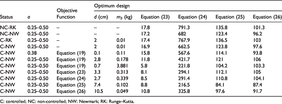
To have a better visualization of the results obtained, a 3-D graph was plotted (Figure 19). In that figure, the maximum structure displacement in function e carved gap (d) and the free mass (m₃) is presented. One can note, analyzing that figure, that the mass varying from 0.2 to 0.3 kg and the gap varying from 2 to 4 cm give the minimum values of displacement. On other hand, one can observe in Table 1, considering equation (25), that the mass varying from 0.05 to 0.3 kg and the carved gap varying from 3 to 10 cm give the minimum values of displacement for all frequencies. It is important to state that the mass is idealized here in the mathematical model as a material point (without dimensions) and the carved gap is the course of the mass.

Figure 19.

Maximum structure displacement as a function e carved gap and the free mass values. (a) Perspective and (b) plan.

Another important observation is that when the free mass is drastically increased and the gap is reduced, the displacements will be reduced too. In a general way, the best values of m₃ varied from 2.5 to 15% of the structure mass and the best value of d varied from 2 to 10 times the static displacement of the structure. However, in problems like the one presented here, where there is a very large range of exciting frequencies (motor frequencies), maybe it should be better to design m₃ and d as a function e frequency and so develop a self-adjusting system for the optimum values obtained as a function e motor frequency. That is, the gap and the free mass assume a given value which depends on the motor frequency.

Conclusions

The Sommerfeld effect and non-ideal dynamic systems were defined. Several types of IDs found in the literature were reported. The equations of motions for the non-ideal system considered here were derived. The augmented Lagrangian method for solving optimization problems with dynamic constraints was presented. Several optimization problems were formulated with the objective to minimize the displacements of the structural system. The design variables of the optimization problems were the free mass and the width of the carved gap of the ID, which were properly varied to obtain the optimum design. Solutions were carried out and the results obtained commented for each optimization problem. Practical designs that reduced the maximum displacements by 50% were obtained. In this work, it was concluded that optimum values of the free mass varied from 2.5 to 15% of the structure mass and the best value of the carved gap varied from 25 to 80 times the static displacement of the structure. The graphs obtained here were compared with those given by the references and the conclusion is that the present formulation presents better results.

Suggestions for further work are as follows:

design an ID in which the free mass and the carved gap are functions of the motor frequency and so develop a system that can be self-adjusted for the optimum values obtained as a function e motor frequency;

optimize an ID with the objective of minimizing the displacements of a wind turbine or a telecommunication tower.

Footnotes

Data availability

All data, samples, models, and code generated or used during the study appear in this article.

Declaration of conflicting interests

The author(s) declared no potential conflicts of interest with respect to the research, authorship, and/or publication of this article.

Funding

The author(s) disclosed receipt of the following financial support for the research, authorship, and/or publication of this article:This work was carried out at the University of São Paulo and Federal University of ABC, in São Paulo, Brazil, and at the University of Iowa, in Iowa City-IA, USA, sponsored by FAPESP under grants No. 2005/02815-5, 2006/04744-0, and 2018/11820-2. All these supports are gratefully acknowledged.

ORCID iD

Alexandre M Wahrhaftig

References

Souza

SLT

Caldas

Balthazar

, et al. Analysis of regular and irregular dynamics of a non-ideal gear-rattling problem. J Braz Soc Mech Sci 2002; 24: 111–114.

Souza

SLT

Caldas

Viana

, et al. Impact dampers for controlling chaos in systems with limited power supply. J Sound Vib 2005; 279: 955–967.

Warminski

Balthazar

Brasil

RMLRF.

Vibrations of a non-ideal parametrically and self-excited model. J Sound Vib 2001; 245: 363–374.

Balthazar

Brasil

RMLRF

Garzeri

FJ.

On non-ideal simple portal frame structural model: experimental results under non-ideal excitation. Appl Mech Mater 2004; 1–2: 51–58.

Mikhlin

Onizhuk

Awrejcewicz

Resonance behavior of the system with a limited power supply having the Mises girder as absorber. J Nonlinear Dyn 2019; 99: 519–536.

Sinha

Bharti

Samantaray

, et al. Sommerfeld effect in an oscillator with a reciprocating mass. Nonlinear Dyn 2018; 93: 1719.

Dimentberg

Mcgovern

Norton

, et al. Dynamics of an unbalanced shaft interacting with a limited power supply. Nonlinear Dyn 1997; 13: 171–187.

Samantaray

AK.

On the nonlinear phenomena due to source loading in rotor-motor systems. J Mech Eng Sci 2008; 223: 809–818.

Samantaray

AK.

Steady-state dynamics of a non-ideal rotor with internal damping and gyroscopic effects. Nonlinear Dyn 2009; 56: 443.

10.

Samantaray

Dasgupta

Bhattacharyya

Sommerfeld effect in rotationally symmetric planar dynamical systems. Int J Eng Sci 2010; 48: 21–36.

11.

Konenko

VO.

Vibrating systems with limited power supply. London: Life Books, 1969.

12.

Bharti

Bisoi

Sinha

, et al. Sommerfeld effect at forward and backward critical speeds in a rigid rotor shaft system with anisotropic supports. J Sound Vib 2019; 442: 330–349.

13.

Quinn

DD.

Resonant dynamics in a rotordynamic system with nonlinear inertial coupling and shaft anisotropy. Nonlinear Dyn 2009; 57: 623–633.

14.

Karthikeyan

Bisoi

Samantaray

, et al. Sommerfeld effect characterization in rotors with non-ideal drive from ideal drive response and power balance. Mech Mach Theory 2015; 91: 269–288.

15.

Balthazar

Mook

Weber

, et al. An overview on non-ideal vibrations. Meccanica 2003; 38: 613–621.

16.

Rocha

Balthazar

Tusset

, et al. An analytical approximated solution and numerical simulations of a non-ideal system with saturation phenomenon. Nonlinear Dyn 2018; 94: 429–442.

17.

Varanis

Balthazar

Silva

, et al. Remarks on the Sommerfeld effect characterization in the wavelet domain. J Vib Control 2019; 25: 98–108.

18.

Popplewell

Bapat

McLachlan

Stable periodic vibroimpacts of an oscillator. J Sound Vib 1983; 87: 41–59.

19.

Bapat

Popplewell

McLachlan

Stable periodic motions of an impact-pair. J Sound Vib 1983; 87: 19–40.

20.

Duncan

Wassgren

Krousgrill

CM.

The damping performance of a single particle impact damper. J Sound Vib 2005; 286: 123–144.

21.

Bapat

Sankar

Single unit impact damper in free and forced vibration. J Sound Vib 1985; 99: 85–94.

22.

Popplewell

Liao

A simple design procedure for optimum impact dampers. J Sound Vib 1991; 146: 519–526.

23.

Saeki

Impact damping with granular materials in a horizontally vibrating system. J Sound Vib 2002; 251: 153–161.

24.

Marhadi

Kinra

VK.

Particle impact damping: effect of mass ratio, material and shape. J Sound Vib 2005; 283: 433–448.

25.

Popplewell

Semercigil

SE.

Performance of a beam bag impact damper for a sinusoidal external force. J Sound Vib 1989; 133: 193–223.

26.

Feitosa

LCS.

Controle por Impacto de Vibrações Estruturais Excitadas por Carregamentos Não-Ideais, Master Dissertation, Polytechnic School of The University of Sao Paulo, Brazil, 2006 (in Portuguese).

27.

Brasil

RMLRF

Feitosa

LCS

Balthazar

JM.

A nonlinear and non-ideal wind generator supporting structure. Appl Mech Mater 2006; 5–6: 433–442.

28.

Brasil

RMLRF

Feitosa

LCS

Balthazar

JM.

Impact control of structural vibrations excited by non-ideal loading. In: Ninth Pan American Congress of Applied Mechanics, Mathematical Sciences Publ, Mérida, Mexico, 2006, p.43.

29.

Arora

Chahande

Paeng

JK.

Multiplier methods for engineering optimization. Int J Numer Methods Eng 1991; 32: 1485–1525.

30.

Chahande

Arora

JS.

Optimization of large structures subjected to dynamic loads with the multiplier method. Int J Numer Methods Eng 1994; 37: 413–430.

Remarks on optimization of impact damping for a non-ideal and nonlinear structural system

Abstract

Keywords

Introduction

IDs

The equations of motion

The augmented Lagrangian method

The optimization problems

Numerical results and comments

Conclusions

Footnotes

Data availability

Declaration of conflicting interests

Funding

ORCID iD

References