
Abstract
A stability analysis for a smart beam with an adaptive controller is presented in the paper when considering the time delay phenomenon. With the Lagrange equation and the assumed modes method, a dynamical model is constructed to describe the hysteresis nonlinearity of the smart beam. By simulation and experiment, the nonlinear model is proved effectively using the strain response near the root of the beam when the piezoelectric actuator is applied on with a chirp voltage. Based on the dynamical model, a stability analysis method is proposed with an eigenmatrix in the discrete control system. Through some simulation verifications, it is concluded that a proper time delay will be useful to improve the stability of the smart beam with an adaptive controller. Furthermore, it is verified by the experiments that the free vibration amplitude of the smart beam with an artificial time delay 0.05 s is smaller compared with that at no time delay.
Introduction
Vibration control problems of various flexible structures by smart materials have been studied for several decades.1–4 In addition, achieving a precise position for the smart structure needs to design a proper controller to suppress the external disturbance. 5 However, the time delay maybe exist in the control system, 6 such as a delayed time considered on a flexible beam by an active vibration absorption method, 7 a delay in going through the sensors and filters, a lag in calculating the control signal in the computer and so on. Therefore, considering the time delay phenomenon in the control system is necessary while the vibration suppression of a smart structure with a controller is studied. Nevertheless, a time delay in the control system may result in instability. Stability must be analyzed when a vibration controller is designed with time delay. 8 Niculescu and Gu presented that the stability of some second-order linear systems with multiple constant and time-varying delays was focused on. 9 Jalili and coworkers conducted that a translational cantilevered Euler–Bernoulli beam with tip mass dynamics at its free end was used for the effect of several damping mechanisms on the stabilization of the beam displacement. 10
For the linear system, Hu and Wang presented the stability analysis of linear damped SDOF vibration control systems with two time delays in the displacement feedback and the velocity feedback, respectively. 11 Nandakumar and Wiercigroch conducted a detailed linear stability analysis of a state dependent delayed coupled two DOF model of drill-string vibration. 12 Furthermore, Nia and Sipahi presented algebraic approaches to design controllers in order to achieve stability regardless of the amount of delays for AVC applications modeled by linear time-invariant systems with “multiple” constant delays. 13 For the nonlinear system, Li et al. 14 proposed a simple algorithm for location the rightmost characteristic root of periodic solutions of some nonlinear oscillators with large time delay. In addition, the stability control domain of beam’s non-linear vibration with time-delay feedback controller was investigated. 15 Therefore, the stability analysis for the smart structure with a controller is an essential task while the vibration suppression of smart structure is studied considering the time delay phenomenon.
Generally, a stability analysis method was studied by calculating eigenvalues of the control system. Singh et al. 16 indicated that a posterior stability analysis was carried out to identify the ranges of the time-delay that maintains the closed-loop assignment while keeping the stability of the infinite number of eigenvalues for the time-delayed systems. Olgac presented that spectral methods were applied to perform a complete stability analysis for a combined system of a delayed resonator absorber and a single degree of freedom mechanical system with a delay in the acceleration feedback. 17 But, the time delay in the control system is not always a negative factor. Naik and Singru 18 described a method to identify the critical forcing function and time delay above which the quarter-car vehicle system became unstable, and the authors found that proper selection of time-delay showed optimum dynamical behavior. Peng et al. presented time-delayed feedback control to reduce the nonlinear resonant vibration of a piezoelectric elastic beam. 19
Before studying the time delay problem, a precise model for the smart structure is necessary. As so far, modeling a smart structure with hysteresis nonlinearity has been researched for many years. For the purpose of controlling vibration for the smart structure, Lee et al. 20 identified a nonlinear rate-independent hysteresis mode-Ishlinskii hysteresis model to investigate vibration control performance. Rodriguez-Fortu et al. adopted the Bouc–Wen model describing the hysteresis between the input voltage V and the charge Q of the piezoelectric actuator to propose a novel active vibration control strategy by adopting a classical sky-hook feedback and a feedforward control. 21 However, it has been increasingly popular that an adaptive control was used to control position for the nonlinear system. The adaptive control is designed with an online identifying model. For example, the multi-channel vibration has been successfully controlled by an adaptive filtered-x LMS algorithm, 22 moreover, a comparison of adaptive sliding mode vibration control with Self Tuning fuzzy logic PID control was implemented for vibration mitigation of nonlinear crane system against earthquake excitations. 23 Therefore, the adaptive control will have an advantage of damping vibration or controlling position in real time for the smart structure under the uncertain environment.
When an adaptive controller is designed, the control law is identified online. The identification control coefficients are obtained by the input and output signals of the control system at the present time and the past time. The output feedback is collected by the sensors. There will be time delay in the feedback signal. When the time delay is large, the control system’s stability may be affected. Even, the control system may have large amplitude vibration with the control signal. This will be harmful to the wider application of the smart structures in different engineering areas.
Therefore, in the paper, considering the hysteresis behavior, a dynamical model for a flexible beam with a piezoelectric actuator is constructed by the Lagrange equation and the assumed mode method. Based on the nonlinear model, an eigenmatrix for the smart beam with an adaptive controller is proposed to analyze the stability of the discrete control system. The adaptive control is adopted with minimum value self-tuning direct regulator (MVSTDR). 24 The MVSTDR for the smart beam with hysteresis nonlinearity is designed online to be having relation with the time delay and the stability of the adaptive control system is analyzed in detail under the time delay environment. Through some simulations, the time delay will affect the stability of the adaptive control system, but an appropriate time delay not only enhances the vibration control effect but also improves the stability for the control system. Finally, it is verified by experiments that the amplitude of the free vibration with a proper artificial time delay is suppressed to a minimum value.
The rest of this paper is organized as follows: a dynamical model for a smart beam is obtained with the nonlinear constitutive equation of piezoelectric material, the Lagrange equation and the assume mode method in Section “Dynamical model.” Stability analysis for the vibration control system in the discrete form is derived in Section “Stability analyses.” Some simulation and experiment results are shown and some discussions are presented in Section “Results and discussions” Finally, some conclusions are given in Section “Conclusions.”
Dynamical model
A smart system shown in Figure 1 is consisted of a flexible beam, a piezoelectric actuator, and a foil gauge. When the tip end of the smart beam suffers from an initial displacement, the strain near the root of beam is collected by the foil gauge and is transmitted to the designed controller for calculating the control voltage applied on the piezoelectric actuator. As a result, with the control voltage, the free vibration will be attenuated in a shorter time. Before the stability is analyzed when considering the time delay in the control system, a dynamical model first will be proposed.
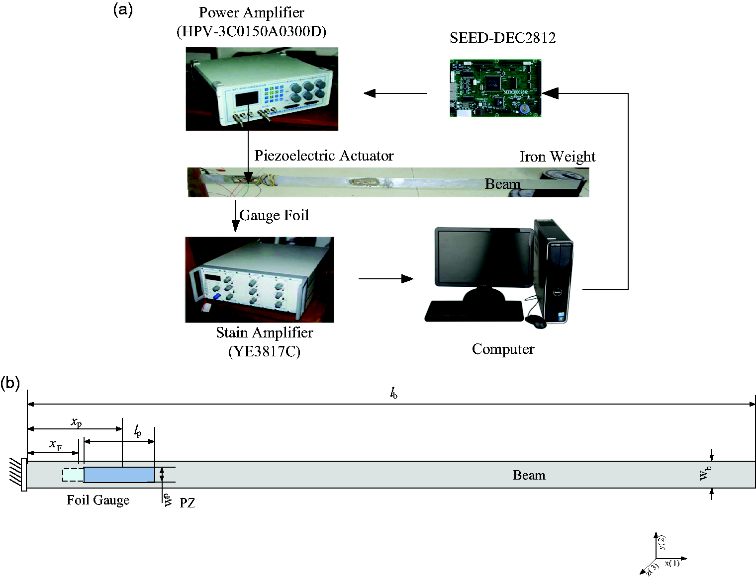
Smart system. (a) Experimental setup of smart system and (b) diagram of smart beam.
Nonlinear constitutive equation of piezoelectric actuator
First, a smart beam system is shown in Figure 1. The smart system is studied for suppressing vibration of cantilevered beam. Figure 1(a) displays an experimental setup of the smart beam. The smart system is consisted of a power amplifier (HPV-3C0150A0300D), a controller (SEED-DEC2812), a computer, strain amplifier (YE3817C) and a smart beam. From Figure 1(b), the displacement
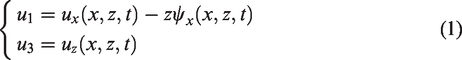
Where
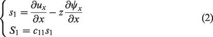
Therefore, the linear constitutive equation of piezoelectric actuator have been widely used as
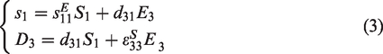
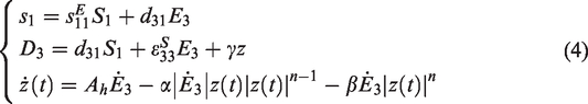
Furthermore, Bouc–Wen equation is a classical hysteresis model, which is proposed by Bouc and Wen for a hysteresis force of a simple spring system. However, the Bouc–Wen equation is employed to describe the hysteresis property between the electric field E and the electric displacement D of the piezoelectric actuator. Therefore, the nonlinear constitutive equation is attained by combining the Bouc–Wen equation with the linear constitutive equation (3) and is expressed as
Dynamically modeling smart beam
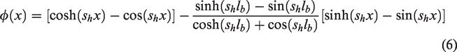
The smart system’s dynamical equation can then be derived using the Lagrange’s equations and the assumed modes method. To suppress the first-order modal vibration of smart beam, the assumed first-order vibration mode

And in equation (5), the assumed mode is
Moreover, when
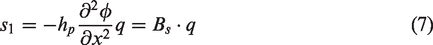
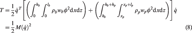
Furthermore, the system energy includes the kinetic energy T, the potential energy U and the work W done by the external force, the damping force and the applied voltage. First, the kinetic energy term
Then, assuming
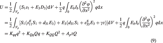
Finally, for the smart beam, its virtual work done by external force
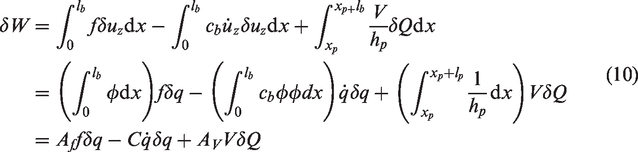
Then, the Lagrange’s equation 25 is described as
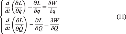
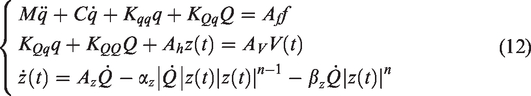
Substituting the equations (8) to (10) into the equation (11), the dynamical model of the smart system is obtained as
Verification of hysteresis model
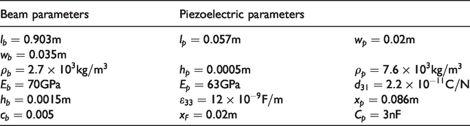
Some simulations and experiments (the experimental setup and the corresponding parameters of the smart beam are shown in Table 1) are implemented to verify the effectiveness of the model for describing the dynamic characteristic and the hysteresis nonlinearity between the input voltage and the out stain by equation (12). From Figures 2 to 5, it is obvious that not only the simulation results but also the experimental data validate the theoretical model of the smart beam.
Dynamical parameters used in simulations.
As is shown in Figure 2, a chirp voltage (150 V × sin(2πf × t), t is time, frequency f = 1.3 + 0.04t) is applied on the piezoelectric actuator when t ≤ 50 s. Then, an output strain signal near the root of the smart beam is acquired and is presented in Figure 3. The amplitude of the strain response is first increasing and then decreasing. Through simulation and experiment strains in Figure 3(a) and (b), respectively, it is indicated that the amplitude of the strain response at time about 10 s achieves its maximum value and then the frequency of the input voltage is about 1.6 Hz.
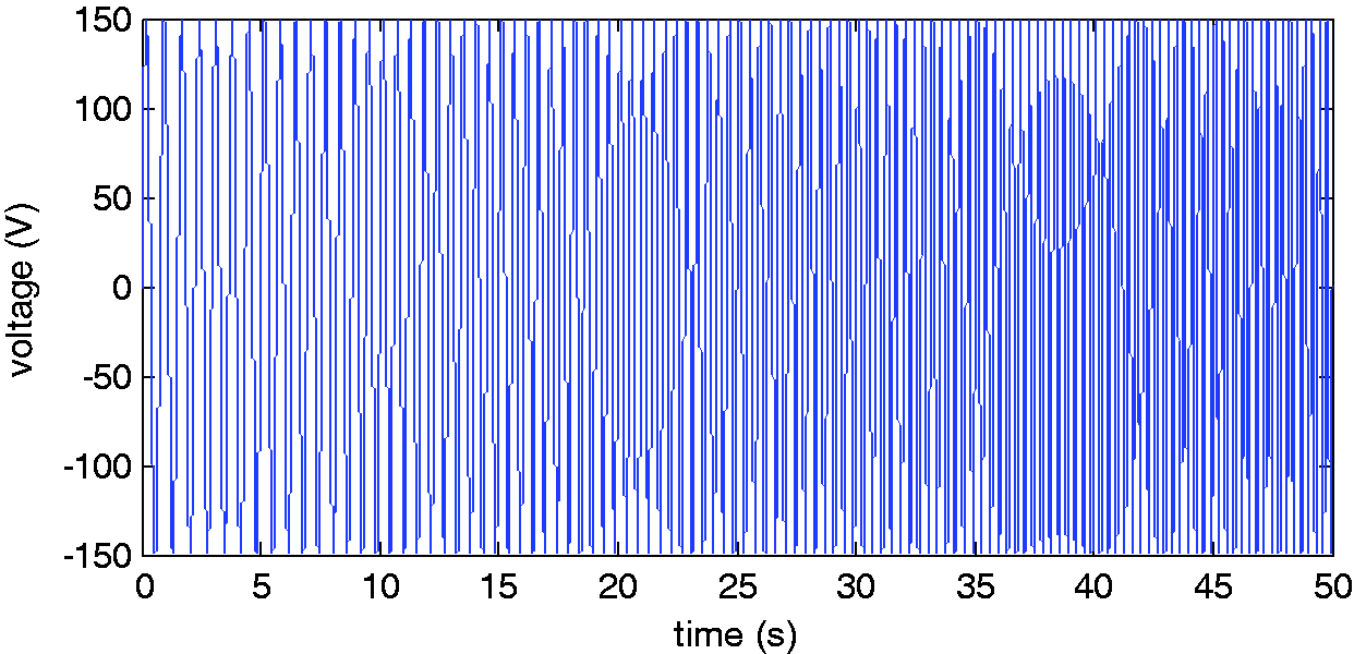
A chirp voltage signal at frequency 1.3–3.3 Hz.
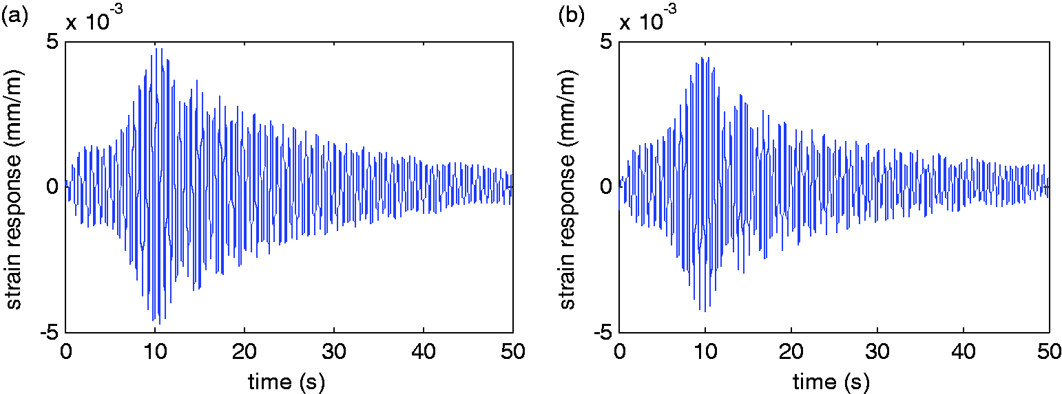
Strain response with a chirp signal voltage. (a) Simulation and (b) experiment.
Furthermore, the strain responses shown in Figure 3 are processed by Fast Fourier Transform (FFT) and their amplitude-frequency characteristics at frequency domain are given in Figure 4. For the Amplitude of frequency response, the peak of the experiment curve is 0.001312 mm/m at frequency 1.563 Hz while the peak of the simulation curve is 0.001357 mm/m at frequency 1.563 Hz. Hence, it is informed that the first natural frequency of the smart beam is about 1.563 Hz. In addition, Figure 5 shows the hysteresis nonlinearity between the input voltage and the strain response when a sinusoidal voltage at amplitude 150 V and frequency 1.56 Hz is applied on the piezoelectric actuator. The simulation data is obtained from the hysteresis model equation (12) while the experiment curve is gained from the practical test. From the two curves in Figure 5, the hysteresis loop of simulation is consistent with that of experiment.
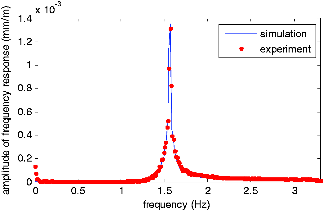
Frequency response.
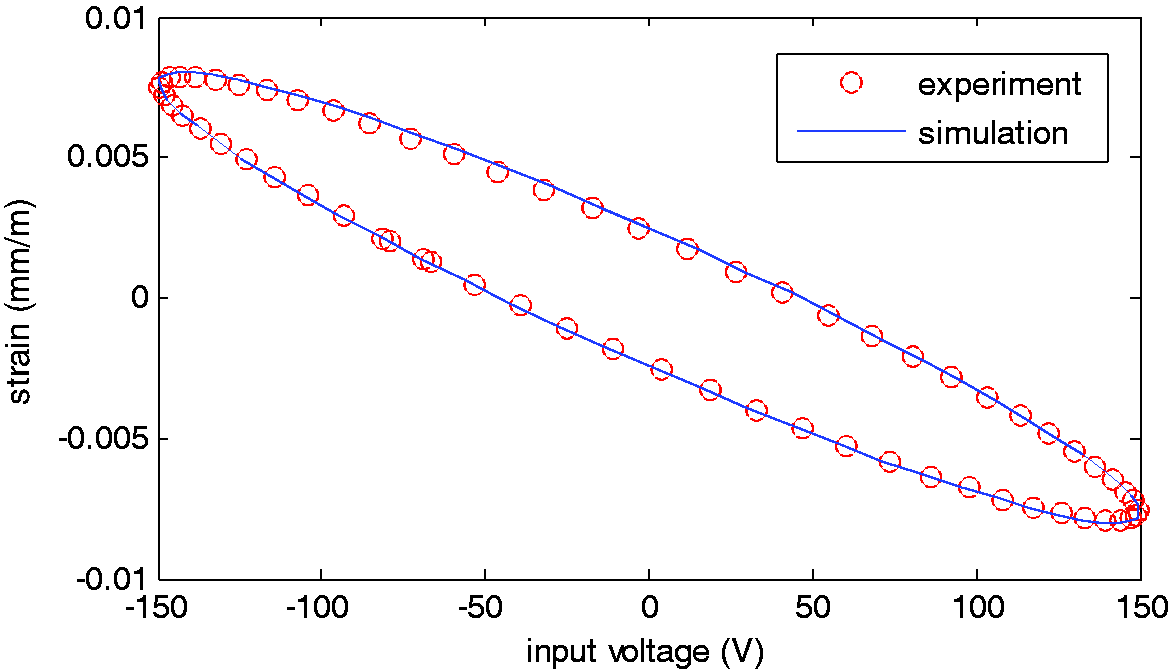
Hysteresis loop at frequency 1.56 Hz.
Through the assumed mode method and the Lagrange equation, a dynamical model for a smart beam is derived to describe the hysteresis loop between the input voltage and the output strain near the root of the beam. With a chirp voltage applied on the piezoelectric actuator, the spectral characteristic at frequency 1.3–3.3 Hz is gained, and it is indicated that the first natural frequency of the smart beam is 1.563 Hz. Furthermore, the simulation and experiment prove it available that the hysteresis behavior of the smart beam is described by the dynamical model with the Bouc–Wen equation.
Stability analyses
When a controller is designed for a system, the time delay appears in the control system and it may have an influence on the stability of the system. Therefore, it is a necessary task to analyze the stability for the vibration control system with time delay. Taking the time delay of the input voltage into account, equation (12) may be transformed to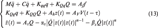
Then, eliminating the variable Q in equation (13), a simplified second-order differential equation is derived as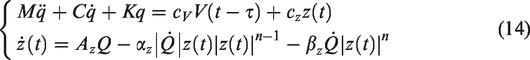
A state space model is gained from the first formula of equation (14) and is expressed as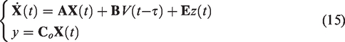
Furthermore, the state equation is resolved and the continuous state vector is given as
When 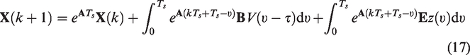
Assuming the time delay 
And assuming 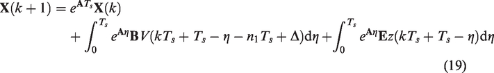
When 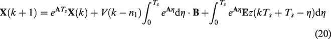
Assuming 
Assuming
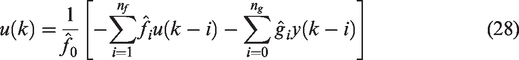
Then, the control voltage in a closed loop control system with time delay is expressed as
Therefore, the extended discretized state vector may be attained as
 where
where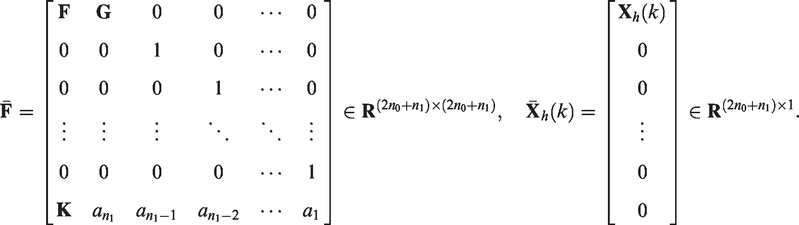
When 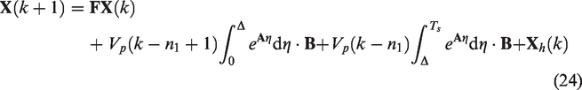
Assuming 
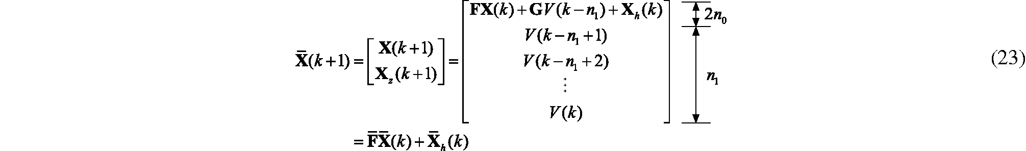
The extended state vector is written as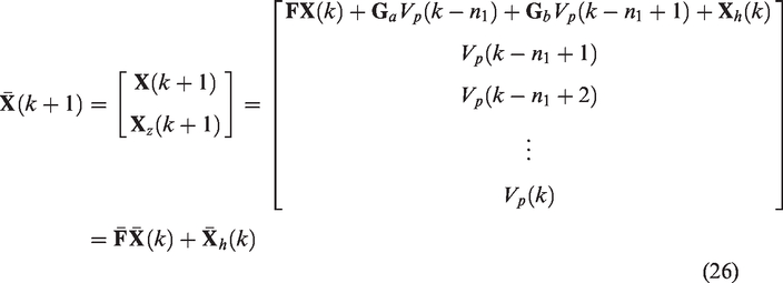
When the stable state 
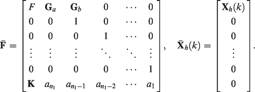
Then,
And
When an artificial time delay is brought into the control system after designing an adaptive controller,
Based on the dynamical model of the smart beam with hysteresis property, a theoretical model with time delay is constructed and is transformed to a simplified second-order differential equation for stability analysis. When the time delay is assumed to be having relation with the sampling rate, an eigenmatrix for the dynamical model with an adaptive controller is proposed to analyze the stability in the discrete system. In the next section, by the stability eigenmatrix, some results and discussions will be given.
Results and discussions
Some necessary simulations and experiments are performed in the Section. The simulations are implemented in the Matlab/Simulink and the experimental setup has been shown in the previous research. The control system is presented in Figure 6. It is indicted that the out strain is collected by a sensor device (a strain gauge) when the tip of the smart beam suffers from an initial displacement (about 10 cm). It will take some time for the strain signal to transmit cross the sensor, the filter, and the controller, which leads to a time delay. In addition, the time delay may be the negative or the positive factor for the stability of the closed loop control system. The system stability is analyzed by calculating the eigenvalues of equation (27). Furthermore, the stability analysis results of the control system with time delay are presented from Figures 7 to 15.
Control system.
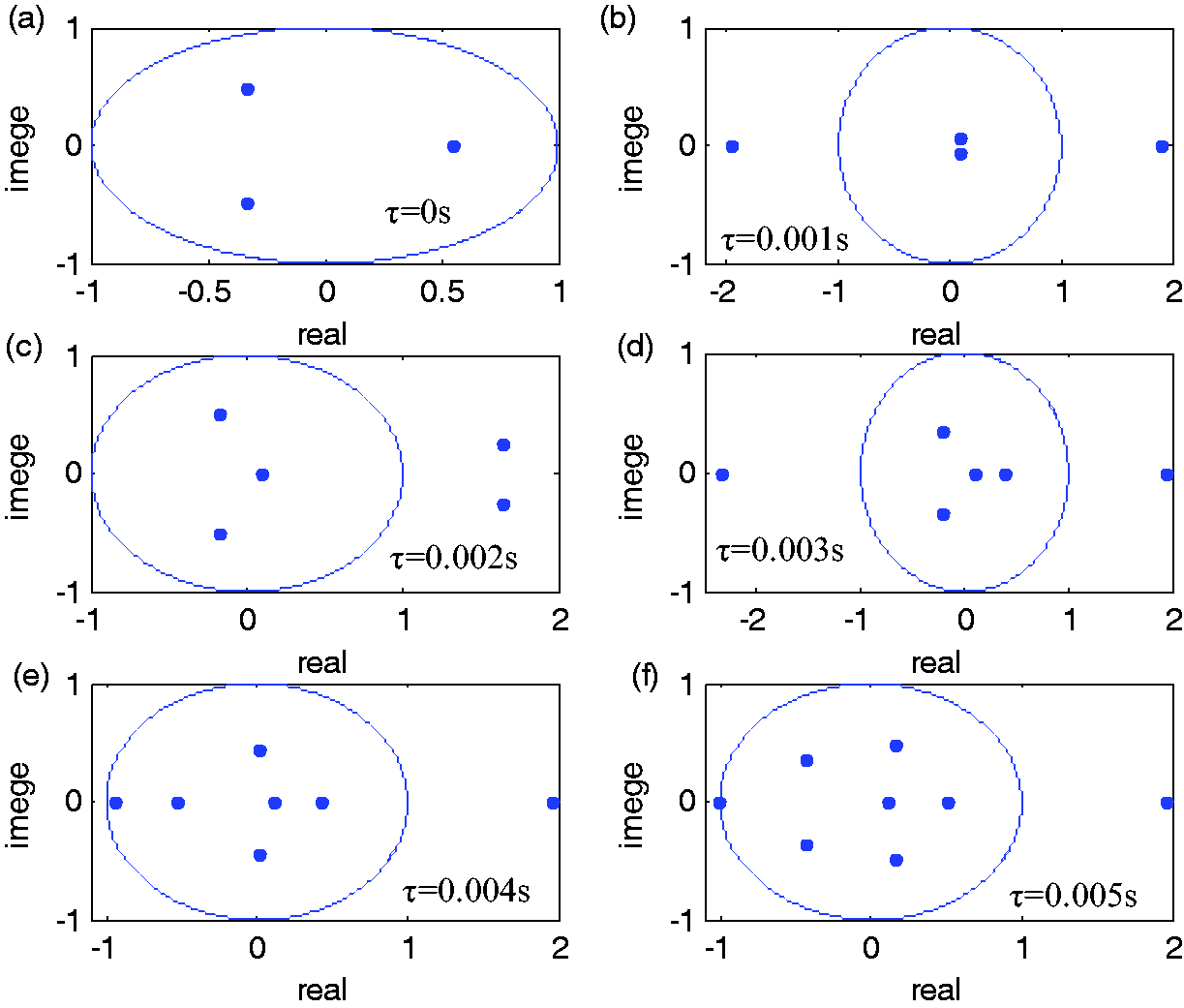
Eigenvalues at τ = 0–0.005 s.
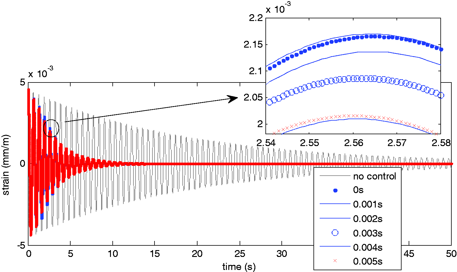
Vibration suppression results at τ = 0–0.005 s.
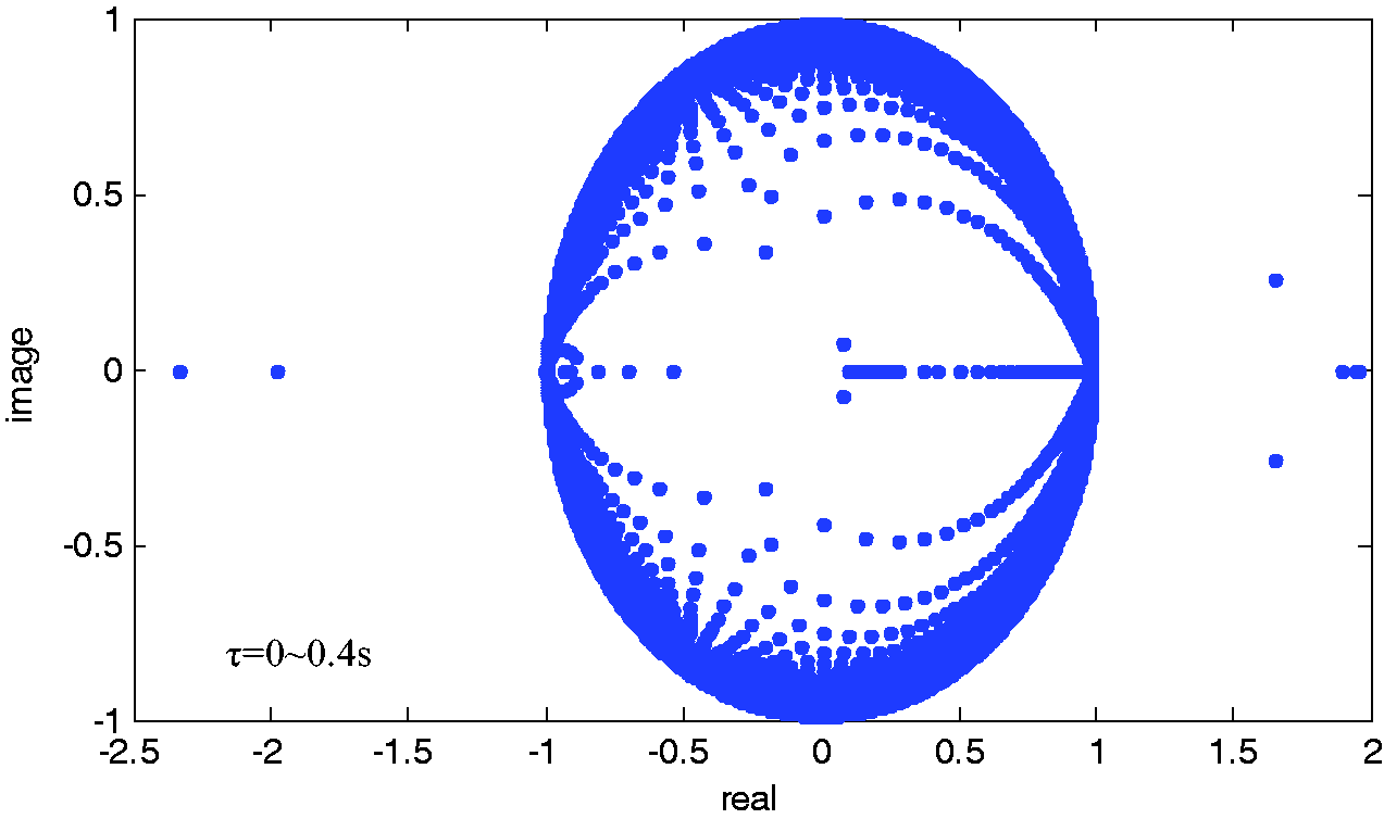
Eigenvalues at τ from 0 s to 0.4 s.
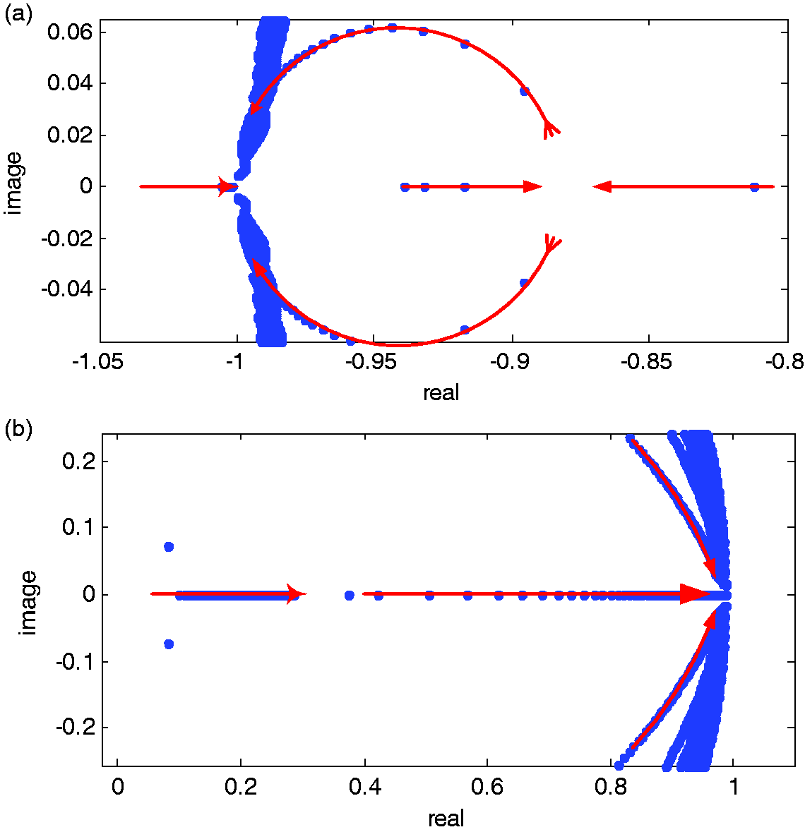
Partial enlargement of Figure 9. (a) Eigenvalues in the side of the negative real axis and (b) Eigenvalues in the side of the positive real axis.
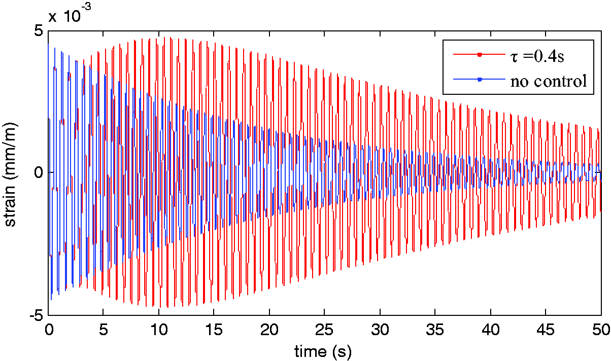
Control result at time delay 0.4 s.
Spectral analysis of vibration suppression results.
Peak of the spectral analyses curve at τ = 0–0.1 s.
Simulation control results at the time delay 0 s 0.05 s, and 0.3 s.
Experimental control results at the time delay 0 s and 0.05 s.
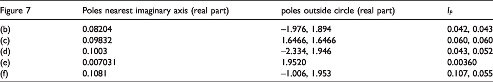
Figure 7 shows the eigenvalues of equation (27) for the smart beam at time delay 0–0.005 s, and the solid lines is the unite circle. When the eigenvalue is in the circle, the corresponding state variable is convergent and the control system is stable. Conversely, if the eigenvalue is out and on the unite circle, the control system is unstable. In Figure 7(a), the eigenvalues are (–0.3346 ± 0.48j and 0.5482) at time delay 0 s and their absolute values are <1, as a results, the state variables are all convergent. As shown in Figure 7(b), the eigenvalues are (–1.976, 0.08204 ± 0.07337j, and 1.894) at time delay 0.001 s, and the corresponding state variables of the two eigenvalues (–1.976 and 1.894) are non-convergent. Figure 7(c) gives the eigenvalues (–0.1828 ± 0.4978j, 0.09832, and 1.6466 ± 0.2554j) at time delay 0.002 s and the state variable of the two eigenvalues (1.6466 ± 0.2554j) are also non-convergent. Figure 7(d) presents the eigenvalues (–2.334, –0.2075 ± 0.3358j, 0.1003, 0.3742, and 1.946) at time delay 0.003 s, then, –2.334 and 1.946 are unstable eigenvalues. Shown in Figure 7(e), the eigenvalues are (–0.9388, –0.5351, 0.007031 ± 0.4434j, 0.1081, 0.4223, 1.9520) at time delay 0.004 s and only an eigenvalue 1.9520 is >1. In Figure 7(f), the eigenvalues are (–1.006, –0.4271 ± 0.3618j, 0.1081, 0.1588 ± 0.484j, 0.5035, 1.953) at time delay 0.005 s, and –1.006 and 1.953 are out of the unite circle.
Based on the eigenvalues at different time delay, the control system with no time delay is stable, as shown Figure 7(a). When the time delay is artificially added into the closed loop, the system becomes unstable. At time delay 0.001 s, 0.002 s, 0.003 s, and 0.005 s in Figure 7(b) to (d) and (f), respectively, there are two unstable eigenvalues (out of the unite circle) per subfigure. And only an eigenvalue is out of unite circle at time delay 0.004 s in Figure 7(e). But, these eigenvalues are non-dominant poles, the non-dominant eigenvalues is defined by three points: The pole is far from the dominant eigenvalues and the imaginary coordinate axis. The absolute value of the real part for the nondominant pole ( When the non-dominant pole is on the real axis, the vibration amplitude caused by the nondominant pole is less compared with that on the imaginary axis.
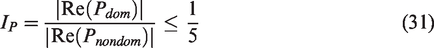
The most relevant factors are not only the number of eigenvalues out of the unit circle but also the real part of the nondominant pole. Therefore, for Figure 7, the ratio
The ratio
If the control system is brought into with a small time delay, the poles outside unite circle are nondominant poles and the pole nearest the imaginary axis is viewed as the dominant pole. When the ratio
Furthermore, at time delay 0.006 s, the eigenvalues are (–0.9318, –0.7011, –0.267 ± 0.5258, 0.1082, 0.2809 ± 0.4906, 0.5665, 1.9530). When the time delay is increasing (0.007, 0.008, 0.009, …, 0.399, 0.4), all eigenvalues are shown in a real-imaginary coordinate of Figure 9. Obviously, when τ > 0.005 s, these eigenvalues are converging to the unite circle. The partial enlargement plot of Figure 9 is given in Figure 10. When the time delay increases from 0 s to 0.4 s, the eigenvalues in the side of the negative real axis finally tend to –1, as shown in Figure 10(a). At the same time, Figure 10(b) presents that the eigenvalues in the side of the positive real axis reach to 0.2636 and 1. In addition, other eigenvalues in the four quadrants and on the imaginary axis are converging to the unite circle.
Therefore, when the time delay gradually increase, the eigenvalues of the control system tend to the unite circle and the state vector is gradually divergent, finally, the free vibration of the smart beam appears large amplitude oscillation. Figure 11 shows the control result at the time delay 0.4 s. It is indicated that the free vibration amplitude with control is larger than that with no control. Furthermore, it is quite clear that increasing the time delay is no longer useful for the vibration suppression.
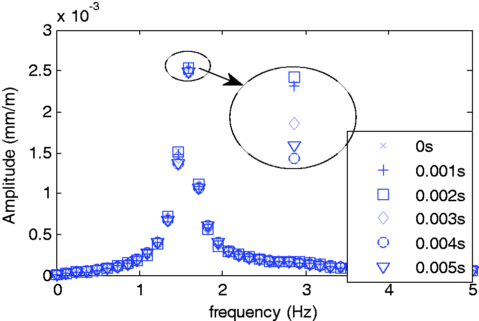
From the view of the spectral analyses, the frequency responses of the control results at the time delay from 0 s to 0.005 s are given by the FFT in Figure 12. The amplitude-frequency curves are presented at frequency from 0 Hz to 5 Hz. It is obvious that the peak of spectral curve at time delay 0.004 s is the smallest, while the curve peak at the time delay 0.002 s is the biggest. Therefore, the control effect at time delay 0.004 s is the best compared with that at other time delay.
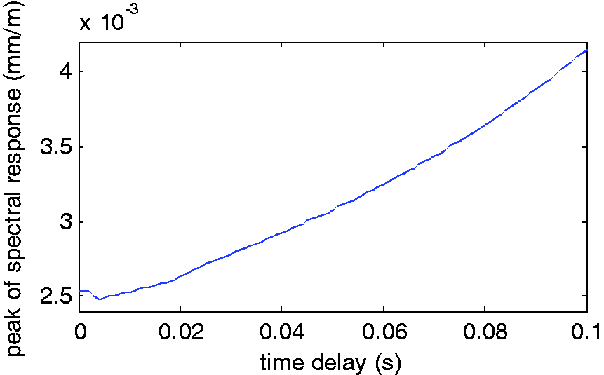
Figure 13 shows the peaks of spectral response curves when the time delay increases from 0 s to 0.1 s. Obviously, with the time delay increasing from 0 s to 0.004 s, the peak at the time delay 0.004 s reaches the minimum value. Then, the peak of spectral response curve is always increasing when the time delay increases from 0.004 s to 0.1 s. Therefore, an enough small time delay not only enhances the system stability but also improves the control effect.
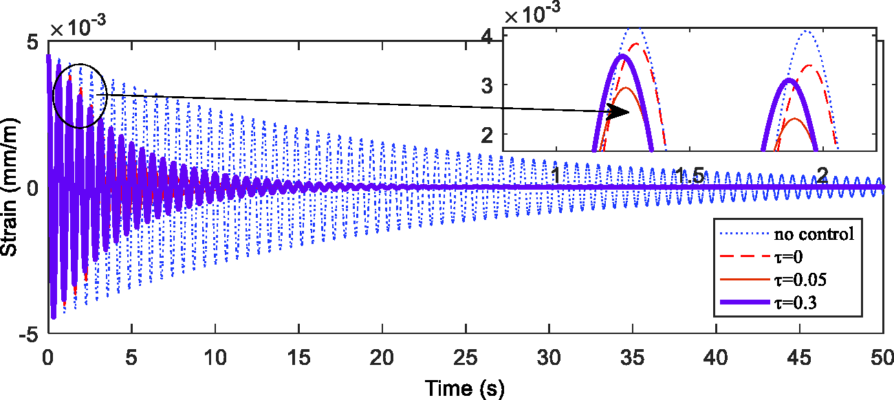
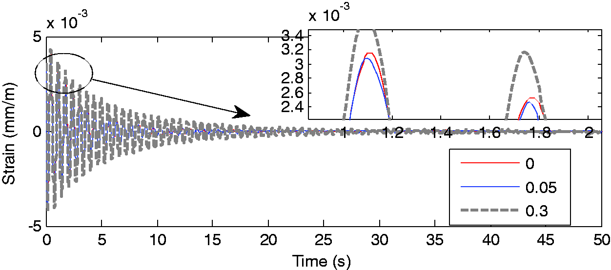
Figure 14 shows simulation results about vibration control at time delay τ = 0 s, 0.05 s, and 0.3 s, the blue dotted curve is the strain response with no control. The red “- - -” curve is the control result with no time delay, the red solid curve is the control result with time delay 0.05 s and the purple line is the control result at time delay 0.3 s. By comparing the four curves, the amplitude of the free vibration at time delay 0.05 s is minimum and the result at no time delay is maximum after the free vibration is applied with a control voltage.
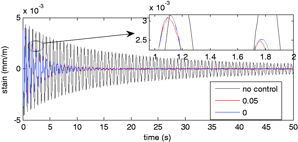
Figure 15 gives the experimental verification of vibration control for a smart beam with a MVSTDR at different time delay with the experiment setup in Figure 1(a). It can be seen in Figure 15 that the free vibration amplitude at time delay 0.05 s is less than that at time delay 0 s when compared with the amplitude of the free vibration with no control. Figure 16 shows the experimental control results at time delay 0 s, 0.05 s, and 0.3 s. It is obvious that the amplitude of strain at 0.3 s is the worst and that at 0.05 is the best. Therefore, it is demonstrated that a proper time delay can enhance the adaptive control performance for the smart system.
Experimental control results at time delay 0 s, 0.05 s, and 0.3 s.
Figure 17 shows the spectral analysis of vibration suppression results at time delay τ = 0 s, 0.05 s, and 0.3 s. It is displayed that the peaks of the spectral curves at time delay τ = 0 s, 0.05 s, 0.3 s, and no control are 0.0003372, 0.0002611, 0.0005319, and 0.002628 (mm/m), respectively. By comparing these peaks of the spectral curves, it is indicated that the peak value of the spectral curve at time delay 0.05 s is the minimum. Therefore, adding a proper time delay into the control system can improve control effectiveness.
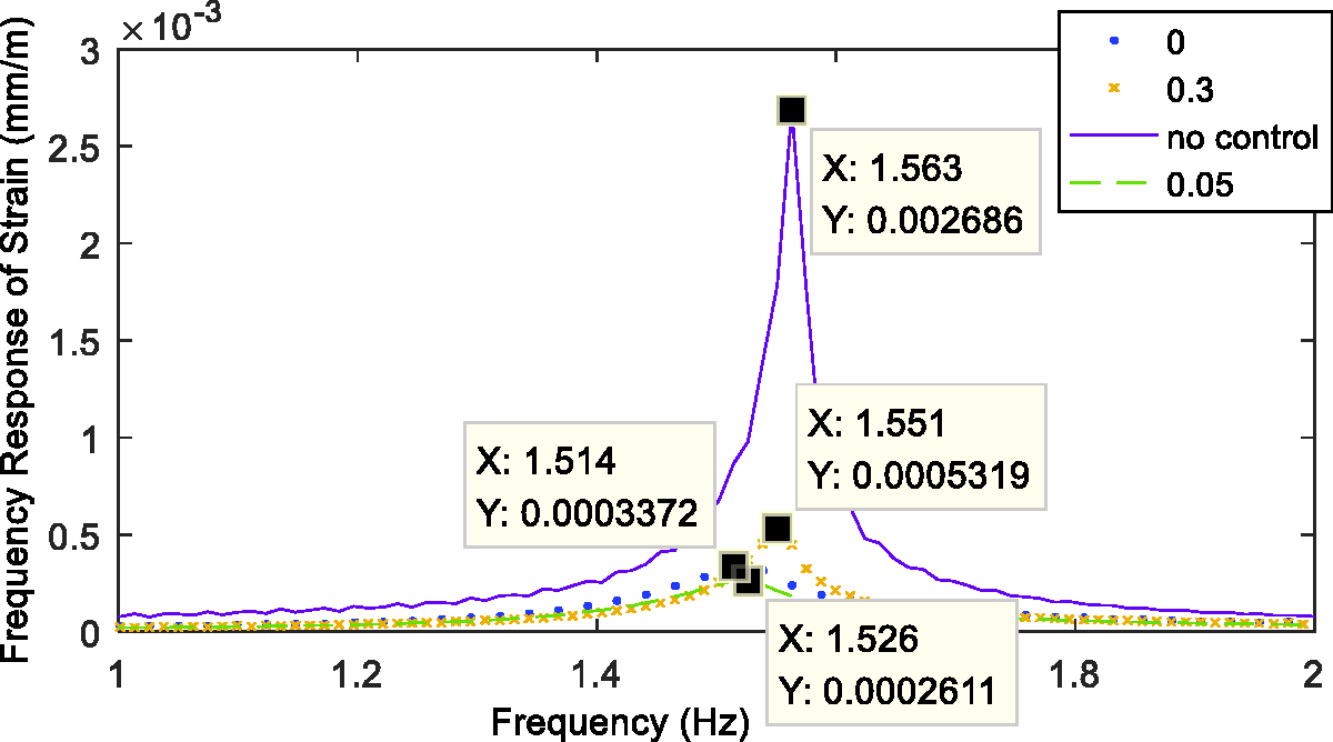
Spectral analysis of vibration suppression results with experiment.
The inconsistency of the time 0.004 s in simulation and the time 0.05 in experiment to achieve the best control effect is due to their different time delays in the system. because there are two factors: One is that the solving differential equations method is adopted with the variable step size ODE45 in the simulation and the variable step size is 0.0009–0.001 s while the step size is fixed in the experiment and the step size is 0.01 s, and this causes simulation system and experimental system have different sampling times; The other is that the time delay in the sensors and the filters is not considered in simulations and this time delay is random and is not measurable. By the two factors, there are different time delays in the simulation system and experiment system.
For the smart beam with an adaptive controller, the time delay phenomenon must exist in the control system. In addition, time delay will affect the system’s stability. Therefore, with some simulations, it is indicated that the unstable eigenvalue number of the control system at time delay 0.004 s is less than that at other time delay. Furthermore, the free vibration amplitude and the spectral curve peak are also less than that with other time delay. Finally, it is verified that the control effect with an enough small time delay is better than that at no time delay through simulation and experiment. In other words, a method is proposed to improve control effect by sacrificing system’s stability with a small time delay to a certain extent, but it is not applicable with a large time delay and the vibration caused by the large time delay is not neglected.
Conclusions
In the paper, a dynamical model of a smart flexible beam with hysteresis nonlinearity is constructed using the assumed modes method and the Lagrange equation, and the theoretical model is verified by simulations and experiments. Based on the dynamical model, an eigenmatrix is derived for analyzing the stability of the smart beam with time delay in the discrete adaptive control system. If the absolute eigenvalues of the eigenmatrix is <1, the control system is stable else its unstable. With the stability analysis results, the time delay has important influence on the stability of the control system. In addition, a proper small time delay is conducive to the stability in the control system. Furthermore, it is proved effectively by simulation and experiment that the control effect can be improved with a small time delay. The next work will focus on studying the specific relation between the adaptive control law and the time delay for the nonlinear system and analyzing the hysteresis influence on the stability of the smart beam after experiment setups are rebuilt.
Footnotes
Declaration of Conflicting Interests
The author(s) declared no potential conflicts of interest with respect to the research, authorship, and/or publication of this article.
Funding
The author(s) disclosed receipt of the following financial support for the research, authorship, and/ or publication of this article: This work was funded by the National Natural Science Foundation of China (NSFC) under No. 11702168, 11602135 and 51605277.