Sage Journals: Discover world-class research

Abstract

This paper proposes the visual servoing resolved acceleration control scheme applied to a 3-degree of freedom (DOF) planar manipulator, which aims to reduce computational loads of the feedback control loop and the tracking errors of the end-effector in the conventional resolved acceleration control scheme. The computation loads are increased due to the calculations of the direct kinematics and the velocity inversion in the feedback control loop. The tracking errors of the end-effector are increased due to low-accuracy encoders, gearbox backlashes, and manipulator flexibility, etc. The proposed scheme incorporates a visual system, which directly captures the position of the end-effector instead of calculating the direct kinematics and the velocity inversion. Due to the requirement of inverse dynamics in the proposed scheme, the transformation of the Jacobian matrices between the passive and active links is imposed to the Euler-Lagrange’s equation so as to derive dynamic equations. In order to show the control performances, three existing torque-based control schemes are also applied to the manipulator. This study investigates the numerical simulations and the experimental validations, and the results show that the proposed scheme can reduce the computation loads and the tracking errors of the end-effector to compare with the three existing schemes.

Keywords

Parallel manipulator resolved acceleration control visual servo

Introduction

Parallel manipulators are essentially closed-loop kinematics chain mechanisms, and an end-effector is linked to the base of the manipulator by several independent kinematics chains. Planar parallel manipulators are useful for manipulating an object on a plane due to high stiffness in nearly all configurations and a high dynamic performance. A 3-RRR planar parallel manipulator is a typical robot arm with 3-DOFs. Due to its broad applications in industry, it is gradually gaining attention in diverse research areas. Gosselin and Angeles investigated the manipulator from a kinematic viewpoint and established four different design criteria to produce designs having optimum characteristics.¹ Lee and Yien investigated the effects of the nonlinearities on the joint motion control for the manipulator by applying a strategy of combined workholding and workhandling to reduce machine setup time.² Gosselin and Sefrioui presented a general solution for the direct kinematic problem for this manipulator using geometric considerations, and this problem leads to a maximum of six real solutions.³ Liu et al. discussed the issue of computer-aided design for the manipulator through the physical model, which can be used systematically to express the relationships between the performance criteria and all link lengths.⁴ Yang et al. focused on the forward singularity analysis of the manipulator and proposed a simple geometric approach based on the concept of instantaneous center.⁵ Geike and McPhee presented an approach to derive kinematic and dynamic equations by using a combination of linear graph theory, the principle of virtual work, and symbolic programming.⁶ Arsenault and Boudreau presented the synthesis of the manipulator using a genetic algorithm.⁷ Oetomo et al. presented the direct kinematic solution of the manipulators, where they are possible to decouple the polynomial further into two quadratic equations, describing the position and orientation of the end-effector, respectively.⁸ Cha et al. presented the singularity avoidance of the manipulator using kinematic redundancy.⁹ Arakelianan and Smith discussed the development of the reactionless manipulators, which apply no reaction forces or moments to the mounting base during motion.¹⁰ Behi et al. presented a microfabricated manipulator with the potential for low-torque precision positioning applications, where the microfabrication process includes the effects of joint clearances, component nonplanarity, and residual-stress-induced linkage deformations.¹¹

Torque control is one of control schemes by sensing motor torques as feedback signals. In robot control, it becomes popular by using current sensors or dynamic models to calculate motor torques instead of directly applying torque sensors. Because of wide applications, torque control has been related to many studies in recent years. He et al. developed an adaptive impedance control for an n-link robotic manipulator with input saturation by employing neural networks, where both uncertainties and input saturation are considered in the tracking control design.¹² Focchi et al. analyzed the stability region of impedance parameters and the passivity of the system influenced by viable range of stable stiffness and damping values of impedance control.¹³ Heshmati-Alamdari et al. presented a model-free control protocol for force controlling of an underwater vehicle manipulator system contacting with an unknown compliant environment, where any knowledge of the system, exogenous disturbances, and sensor’s noise model are unknown.¹⁴ Yue et al. studied the speed control of a permanent magnet synchronous motor with the direct torque control scheme and Speed Vector Pulse Width Modulation (SVPWM), where the fractional order calculus theory is used to design the fractional order proportional–integral–derivative (PID) controller.¹⁵ Sangdani applied an optimal control scheme based on genetic algorithm to a tracker robot with machine vision, and the experimental results revealed the effectiveness of the controller and confirmed the stability of the system.¹⁶ Rani and Kumar proposed a hybrid position/force control scheme for coordinated multiple mobile manipulators holding a rigid object, where the inefficiency of the model-based controller is recovered by combining with a neural network based controller.¹⁷ Kumar et al. investigated three intelligent computed torque control (CTC) schemes applied to a 3-DOF robotic manipulator, where the three control schemes are computed torque proportional-derivative control, computed torque fuzzy logic control, and computed torque adaptive network fuzzy inference system.¹⁸

Resolved acceleration control (RAC) is a kind of torque control, the concept of which was proposed by Luh et al. in 1980,¹⁹ and the concept was further modified as the approach of resolved-motion-rate.²⁰ In addition to directly deal with the position and direction of the end-effector, it is also necessary to have the prescribed acceleration command. Noshadi et al. presented an intelligent control scheme to track accurately a prescribed trajectory for the system with disturbances, where a two-level fuzzy tuning RAC is applied.²¹ The RAC method involves velocity conversion. When a robot manipulator reaches singular points, the inverse Jacobian matrix does not exist, and this causes the RAC controller to diverge. Thus, Wu and Lin proposed an improved method which is damped-acceleration resolved-acceleration control (DARAC).²² However, the DARAC may cause the trajectory to fluctuate at the end-effector when the joint speed is nonzero, so they propose a modified method damped-rate resolved-acceleration control to solve the singularity problem.^23,24 Followed by the pioneers’ work, there are more research works focusing on the applications of the RAC. Ambar et al. applied the RAC to a dual-arm underwater vehicle system, where the robotic arms and the vehicle are coordinated controlled by considering the effects of hydrodynamic forces.²⁵ Nakano et al. also investigated the RAC of an underwater robot with three-link dual arms by using position and velocity feedbacks from the vehicle and the end-tip of the arms, and the results were compared with those by applying the CTC.²⁶

Visual servo control is a control method by extracting information from images captured by a vision sensor and delivering back to a controller. Recently, there are more applications on visual servo control. Hutchinson et al. provided a tutorial introduction to visual servo control of robotic manipulators.²⁷ Besides, Chaumette and Hutchinson presented visual servo control using computer vision data in the servo loop to control the motion of a robot.^28,29 Tsai et al. applied visual servo control to a 5-DOF robot manipulator to perform pick-and-place tasks, where a hybrid switched reactive-based visual servo control structure is proposed.³⁰ Serra et al. presented the landing problem of a vertical take-off and landing vehicle for a quadrotor on a moving platform using image-based visual servo control, and the control law can guarantee convergence to the desired landing spot.³¹ Wang et al. proposed an adaptive visual servo controller for soft manipulators contacting with constrained environments, where the controller is based on piecewise-constant curvature kinematics and does not need the manipulator’s length and the target positions.³² Since image processing techniques can directly obtain the position information of the end-effector of robots, there are more research works addressing visual servo control applied to the robot arms. Wang et al. proposed an adaptive neural network control for visual servoing robotic system, where the unmodeled dynamics and output nonlinearity are taken into account.³³ Feng et al. proposed a robot system with visual servo control and applied to laparoendoscopic single‐site surgery, where an uncalibrated visual servo control method is used to have an accurate positioning capability.³⁴

The major disadvantage of the RAC needs more computations due to the complexity of the control scheme, so it might yield worse control performances in experimental implementations. Besides, the RAC regulates the angular accelerations of the position of the end-effector, and the position is calculated through direct kinematics. Thus, the correct position might be not obtained. To solve the two problems, this paper proposes a visual servoing RAC (VSRAC), which aims to directly acquire the position of the end-effector and to reduce computations. Furthermore, the RAC requires the inverse dynamics to calculate the motor torques, and it is difficult to have dynamic models for parallel manipulators due to the complicated derivations. This paper also presents an approach by imposing the Jacobian matrices relating the passive and active links into the Euler-Lagrange’s equation so as to derive the dynamic equations. The rest of this paper is organized as follows. First, the kinematics and dynamics of a 3-DOF planar parallel manipulator is presented, where the dynamics is derived by applying the proposed scheme. Secondly, several torque-based control schemes are introduced, where the proposed VSRAC scheme is presented in details. Thirdly, the experimental setup and the experimental results are presented. Finally, some conclusions are presented.

A 3-DOF planar parallel manipulator

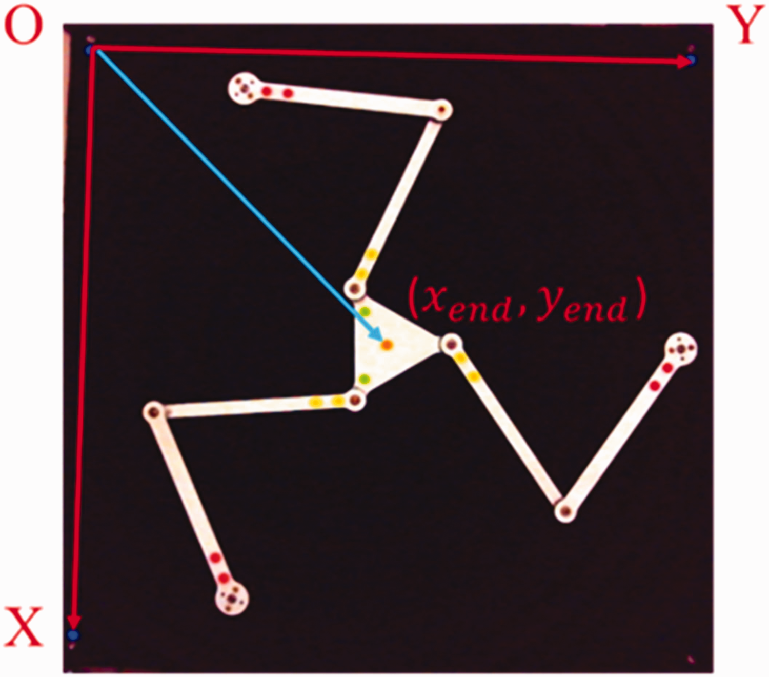
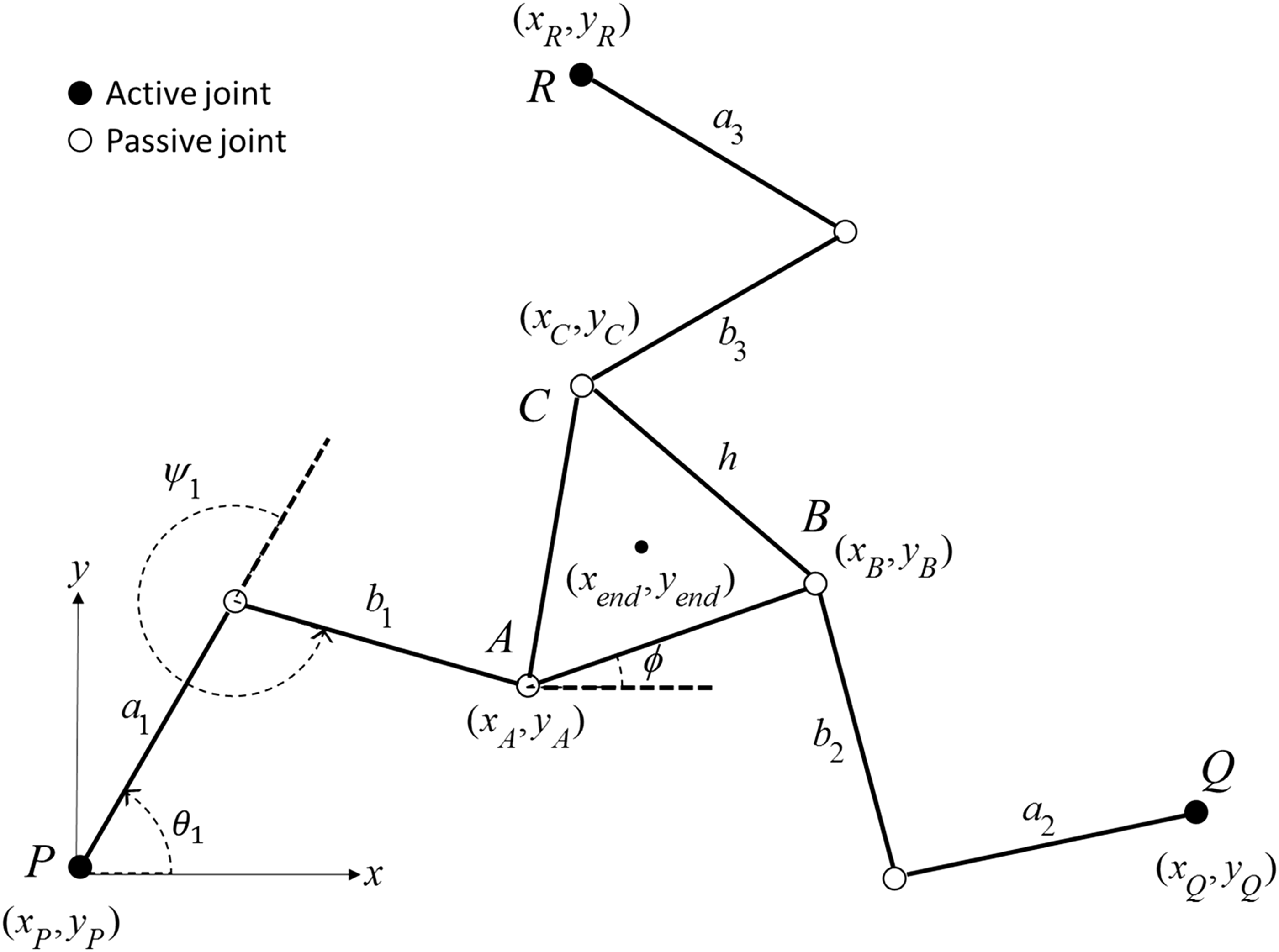
A 3-DOF planar parallel manipulator shown in Figure 1 is driven by three motors fixedly located at coordinates $(x_{P}, y_{P})$ , $(x_{Q}, y_{Q})$ , and $(x_{R}, y_{R})$ , where the origin of an inertial coordinate system is defined at coordinate $(x_{P}, y_{P})$ . The end-effector of the manipulator is referred as the triangle formed by coordinates $(x_{A}, y_{A})$ , $(x_{B}, y_{B})$ , and $(x_{C}, y_{C})$ . The manipulator has three kinematic chains, where each one consists of two links connected from the motor to the end-effector by using revolute joints. The links connected with the motors and the end-effector are called active links and passive links, respectively. The joints are driven by the motors are called active joints, and the other joints are called passive joints.

Figure 1.

A 3-DOF planar parallel manipulator.

Kinematics of the manipulator

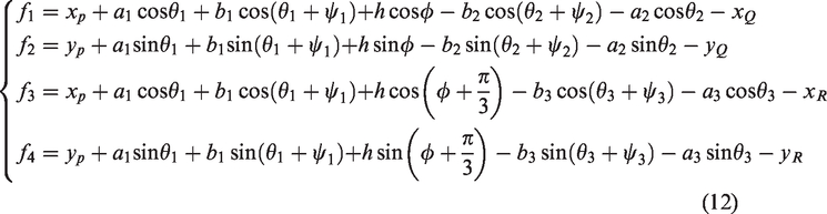
To construct the kinematics of the manipulator, one considers the kinematic chain from coordinates $(x_{P}, y_{P})$ to $(x_{A}, y_{A})$ . Based on the geometry of the manipulator, the identity equations are obtained as³⁵

x_{A} = x_{p} + a_{1} \cos θ_{1} + b_{1} \cos (θ_{1} + ψ_{1})

(1)

y_{A} = y_{p} + a_{1} sin θ_{1} + b_{1} sin (θ_{1} + ψ_{1})

(2)

where

a_{1}

and

b_{1}

are the lengths of the two links of the kinematic chain;

θ_{1}

and

ψ_{1}

are the inclination angles of the two links; the subscript 1 refers to the first kinematic chain.

Summing the squares of this two equations shown in equations (1) and (2) yields

x_{A}^{2} + y_{A}^{2} - 2 x_{A} a_{1} \cos θ_{1} - 2 y_{A} a_{1} sin θ_{1} + a_{1}^{2} - b_{1}^{2} = 0

(3)

Similarly, two additional equations referring to the other two kinematic chains can be derived as

\begin{array}{l} x_{A}^{2} + y_{A}^{2} - 2 x_{A} x_{Q} - 2 y_{A} y_{Q} + x_{Q}^{2} + y_{Q}^{2} + h^{2} + a_{2}^{2} - b_{2}^{2} + 2 x_{A} h \cos ϕ + 2 y_{A} h sin ϕ \\ - 2 x_{A} a_{2} \cos θ_{2} - 2 y_{A} a_{2} sin θ_{2} - 2 x_{Q} h \cos ϕ - 2 y_{Q} h sin ϕ + 2 x_{Q} a_{2} \cos θ_{2} \\ + 2 y_{Q} a_{2} sin θ_{2} - 2 l_{a 2} h \cos ϕ \cos θ_{2} - 2 a_{2} h sin ϕ sin θ_{2} = 0 \end{array}

(4)

\begin{array}{l} x_{A}^{2} + y_{A}^{2} - 2 x_{A} x_{R} - 2 y_{A} y_{R} + x_{R}^{2} + y_{R}^{2} + h^{2} + a_{3}^{2} - b_{3}^{2} + 2 x_{A} h \cos (ϕ + \frac{π}{3}) \\ + 2 y_{A} h sin (ϕ + \frac{π}{3}) - 2 x_{A} a_{3} \cos θ_{3} - 2 y_{A} a_{3} sin θ_{3} - 2 x_{R} h \cos (ϕ + \frac{π}{3}) - 2 y_{R} h sin (ϕ + \frac{π}{3}) \\ + 2 x_{R} a_{3} \cos θ_{3} + 2 y_{R} a_{3} sin θ_{3} - 2 a_{3} h \cos (ϕ + \frac{π}{3}) \cos θ_{3} - 2 a_{3} h sin (ϕ + \frac{π}{3}) sin θ_{3} = 0 \end{array}

(5)

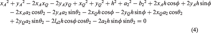
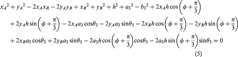
Therefore, equations (3), (4), and (5) describe the relationship of the rotating angles $(θ_{1}, θ_{2}, θ_{3})$ of the motors and the position and the orientation angle $(x_{A}, y_{A}, ϕ)$ of the end-effector. If the angles $(θ_{1}, θ_{2}, θ_{3})$ are given, it is called the direct kinematics to determine $(x_{A}, y_{A}, ϕ)$ . On the contrary, it is called the inverse kinematics. The detailed derivations of the direct and inverse kinematics can be referred in the study by Tsai.³⁵ Since the velocity and acceleration inversions will be applied in the proposed control scheme presented in next section, it is necessary to derive them by simply differentiating equations (3), (4), and (5) with respect to time, and then they are obtained as

J \dot{x} = \dot{θ}, J \ddot{x} + \dot{J} \dot{x} = \ddot{θ}

(6)

where

J

is a Jacobian matrix in terms of

(x_{A}, y_{A}, ϕ)

and

(θ_{1}, θ_{2}, θ_{3})

;

x

and

θ

represent two vectors written as

{[x_{A} y_{A} ϕ]}^{T}

and

{[θ_{1} θ_{2} θ_{3}]}^{T}

, respectively.

Dynamics of the manipulator

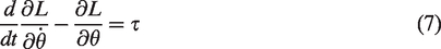
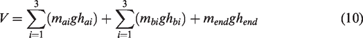
It is difficult to derive the dynamics models of parallel manipulators due to the complexity of derivations. One presents an approach, which imposes the Jacobian matrices relating the passive and active links into the Euler-Lagrang’e equation. Thus, the dynamics of the manipulator is first obtained by using the Euler-Lagrange’s equation as

\frac{d}{dt} \frac{\partial L}{\partial \dot{θ}} - \frac{\partial L}{\partial θ} = τ

(7)

where

θ

is a vector composing the three active angles;

τ

is the torque applied on the active joint; L is the Lagrangian defined as

L = T - V

(8)

in which T and V are the kinetic energy and the potential energy, respectively, which are written as

T = \sum_{i = 1}^{3} \frac{1}{2} (m_{ai} v_{ai}^{2} + J_{ai} {\dot{θ}}_{i}^{2}) + \sum_{i = 1}^{3} \frac{1}{2} (m_{bi} v_{bi}^{2} + J_{bi} {\dot{ψ}}_{i}^{2}) + \frac{1}{2} (m_{end} v_{end}^{2} + J_{end} {\dot{ϕ}}^{2})

(9)

V = \sum_{i = 1}^{3} (m_{ai} g h_{ai}) + \sum_{i = 1}^{3} (m_{bi} g h_{bi}) + m_{end} g h_{end}

(10)

where

m_{ai}

is the masses of active links;

v_{ai}

is the velocities of active links;

J_{ai}

is the moments of inertia of the active links;

h_{ai}

is the height of the active links;

θ_{i}

is the active angles;

m_{bi}

is the mass of passive links;

v_{bi}

are the velocities of passive links;

J_{bi}

are the moments of inertia of the passive links;

h_{bi}

are the heights of the passive links;

ψ_{i}

are the passive angles;

m_{end}

is the mass of the end-effector;

v_{end}

is the velocity of the end-effector;

J_{end}

is the moment of inertia of the end-effector;

h_{end}

is the height of the end-effector;

ϕ

is the rotating angle of the end-effector;

g

is the gravitational constant; the subscript

i

refers to ith kinematic chain; the subscript a and b refer to the active and passive links, respectively; subscript end refers to the end-effector.

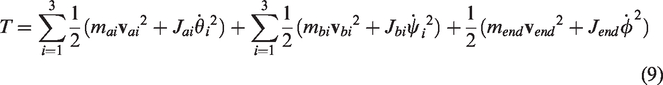
From equation (9), one notes that the kinetic energies of the passive links and the end-effector are functions of their own velocities, but the differentiations for applying the Euler-Lagrange’s equation are with respect to the velocities of the active links. Therefore, it is necessary to have the partial derivatives $\frac{\partial ψ_{i}}{\partial θ_{j}}$ (i, j = 1, 2, 3) and $\frac{\partial ϕ}{\partial θ_{j}}$ in order to apply the chain rules to the formulations of the Euler-Lagrange’s equation. The partial derivatives can be obtained by considering the geometry of the two kinematic chains formed by points PAQ and PAR, and then the x- and y-components of each chain can be expressed as a general form

f_{k} (ψ_{i}, θ_{j}) = 0, (i = 1, 2, 3, 4; j = 1, 2, 3; k = 1, 2, 3, 4)

(11)

where

{\begin{cases} f_{1} = x_{p} + a_{1} \cos θ_{1} + b_{1} \cos (θ_{1} + ψ_{1}) + h \cos ϕ - b_{2} \cos (θ_{2} + ψ_{2}) - a_{2} \cos θ_{2} - x_{Q} \\ f_{2} = y_{p} + a_{1} \sin θ_{1} + b_{1} \sin (θ_{1} + ψ_{1}) + h sin ϕ - b_{2} \sin (θ_{2} + ψ_{2}) - a_{2} \sin θ_{2} - y_{Q} \\ f_{3} = x_{p} + a_{1} \cos θ_{1} + b_{1} \cos (θ_{1} + ψ_{1}) + h \cos (ϕ + \frac{π}{3}) - b_{3} \cos (θ_{3} + ψ_{3}) - a_{3} \cos θ_{3} - x_{R} \\ f_{4} = y_{p} + a_{1} \sin θ_{1} + b_{1} \sin (θ_{1} + ψ_{1}) + h \sin (ϕ + \frac{π}{3}) - b_{3} \sin (θ_{3} + ψ_{3}) - a_{3} \sin θ_{3} - y_{R} \end{cases}

(12)

in which

ψ_{4}

is defined as

ϕ

so as to incorporate it in a vector consisting of the passive angles.

Differentiating equation (11) with respect to time leads to

J_{θ} \dot{θ} + J_{ψ} \dot{ψ} = 0

(13)

where

\begin{array}{l} \dot{θ} = {[\begin{matrix} θ_{1} & θ_{2} & θ_{3} \end{matrix}]}^{T}, \dot{ψ} = {[\begin{matrix} {\dot{ψ}}_{1} & {\dot{ψ}}_{2} & {\dot{ψ}}_{3} & {\dot{ψ}}_{4} \end{matrix}]}^{T}, J_{ψ} = [\begin{matrix} \frac{\partial f_{1}}{\partial ψ_{1}} & \frac{\partial f_{1}}{\partial ψ_{2}} & \frac{\partial f_{1}}{\partial ψ_{3}} & \frac{\partial f_{1}}{\partial ϕ} \\ \frac{\partial f_{2}}{\partial ψ_{1}} & \frac{\partial f_{2}}{\partial ψ_{2}} & \frac{\partial f_{2}}{\partial ψ_{3}} & \frac{\partial f_{2}}{\partial ϕ} \\ \frac{\partial f_{3}}{\partial ψ_{1}} & \frac{\partial f_{3}}{\partial ψ_{2}} & \frac{\partial f_{3}}{\partial ψ_{3}} & \frac{\partial f_{3}}{\partial ϕ} \\ \frac{\partial f_{4}}{\partial ψ_{1}} & \frac{\partial f_{4}}{\partial ψ_{2}} & \frac{\partial f_{4}}{\partial ψ_{3}} & \frac{\partial f_{4}}{\partial ϕ} \end{matrix}], J_{θ} = [\begin{matrix} \frac{\partial f_{1}}{\partial θ_{1}} & \frac{\partial f_{1}}{\partial θ_{2}} & \frac{\partial f_{1}}{\partial θ_{3}} \\ \frac{\partial f_{2}}{\partial θ_{1}} & \frac{\partial f_{2}}{\partial θ_{2}} & \frac{\partial f_{2}}{\partial θ_{3}} \\ \frac{\partial f_{3}}{\partial θ_{1}} & \frac{\partial f_{3}}{\partial θ_{2}} & \frac{\partial f_{3}}{\partial θ_{3}} \\ \frac{\partial f_{4}}{\partial θ_{1}} & \frac{\partial f_{4}}{\partial θ_{2}} & \frac{\partial f_{4}}{\partial θ_{3}} \end{matrix}] \end{array}

(14)

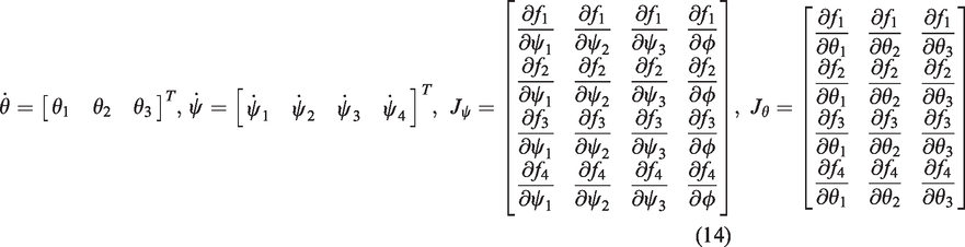
Equation (13) can be further arranged as

\dot{ψ} = - J_{ψ}^{- 1} J_{θ} \dot{θ}

(15)

Alternatively, since the passive angles and the inclination angle are functions of the active angles, the time derivatives of the passive angles and the inclination angle are given as

\dot{ψ} = P \dot{θ}

(16)

where

P_{ij} = \frac{\partial ψ_{i}}{\partial θ_{j}}

Thus, the equality of equations (15) and (16) leads to

\frac{\partial ψ_{i}}{\partial θ_{j}} = - \sum_{k = 1}^{4} (\frac{\partial f_{k}}{\partial θ_{j}}) / (\frac{\partial f_{k}}{\partial ψ_{i}})

(17)

Equation (17) can be used to determine the differentiations in the formulations of the Euler-Lagrange’s equation and then the dynamic equations of the manipulator can be obtained as^8–10

M (θ) \ddot{θ} + C (θ, \dot{θ}) \dot{θ} + H (θ) + B (\dot{θ}) = τ

(18)

where M and C are two matrix functions; H and B are two vector functions referring to the gravitational effects and viscous damping, respectively, and B is an imposing term and does not come from the Lagrangian;

τ

is a torque vector. Equation (18) is the dynamic equation of the manipulator. If the control torque

τ

is known, it is called the direct dynamics by integrating the equation with initial conditions to obtain

θ

. On the contrary, if

θ

\dot{θ}

and

\ddot{θ}

are known, it is called the inverse dynamics to compute the control torque

τ

. The dynamic model will be applied to the following motion control schemes.

Torque-based control schemes

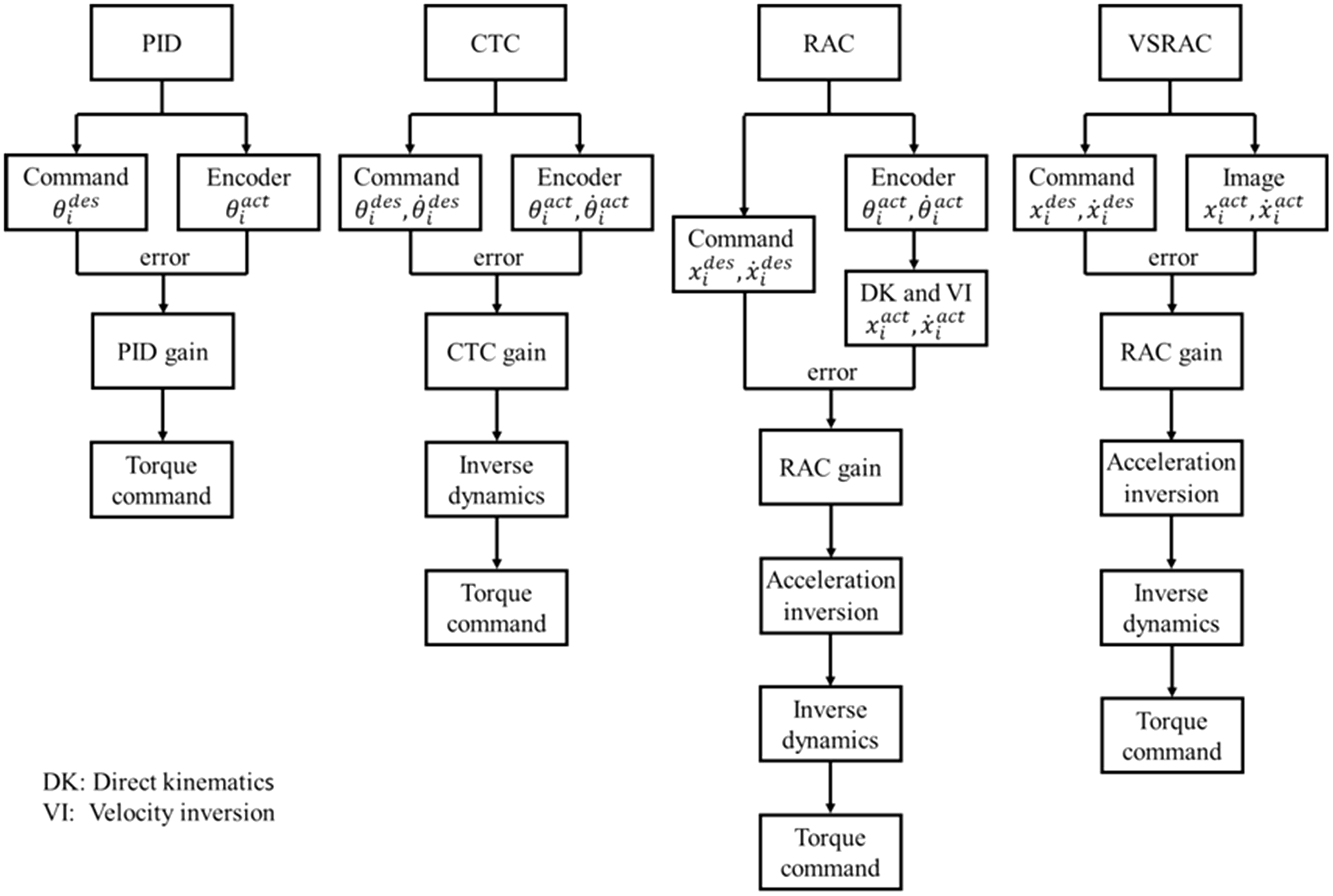
The controllers of the torque-based control schemes will generate desired control torques for motors, and encoders will sense the motor angles and deliver back to the controllers to fulfill the feedback control. Based on this idea, it is necessary to have two feedback loops in the control schemes. The inner loop deals with the torque control of motors, where the motor currents will be sensed by current sensors, and then the currents will be multiplied by the current constants so as to obtain the motor torques. The outer loop deals with the regulations of the angular accelerations of the motors or the accelerations of the end-effector, which depend on the selection of the torque-based control schemes.

This paper proposes a VSRAC, which is a torque-based control scheme. In order to compare the scheme with other existing torque-based control schemes, this section also presents a PID control, a RAC, and a CTC. A torque-based control scheme usually incorporates the dynamic model of manipulators so as to evaluate the control torques instead of directly using torque sensors to measure the torques, so the input signals of the manipulators are the control torques. For different types of control schemes, the feedback signals can be angles of active links or the position and the orientation of the end-effector, so the sensors will be encoders or cameras, respectively.

In order to perform torque-based control schemes, one introduces the torque control of motors first, followed by three existing torque-based schemes, and then presents a VSRAC scheme.

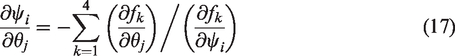
Torque control of motors

To illustrate the torque-based control, Figure 2 shows the block diagram of the torque control for a single motor, where a desired torque $τ_{des}$ divided by the current constant $K_{T}$ of the motor becomes the desired motor current $I_{des}$ , so the toque control problem of a motor is converted to a current control problem. Besides, a current sensor is used to sense the motor current, which is sent to the PID controller given as

I_{ref} = K_{p}^{T} e_{I} + K_{i}^{T} \int e_{I} d t + K_{d}^{T} {\dot{e}}_{I}

(19)

where

K_{p}^{T}

K_{i}^{T}

, and

K_{d}^{T}

are the PID controller gains for the torque control of a motor;

e_{I}

is the error of the desired current

I_{des}

and the actual current

I_{act}

e_{I} = I_{des} - I_{act}

(20)

Figure 2.

Block diagram of the torque control for a single motor.

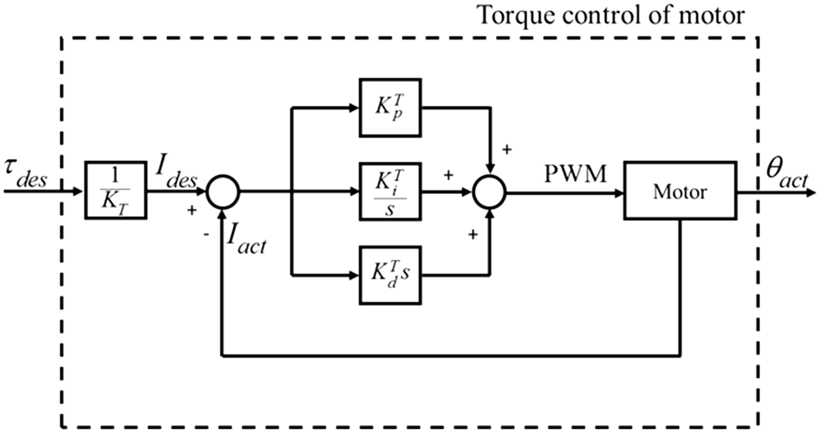
Proportional-integral-derivative control

Figure 3 shows the block diagram of a proportional-integral-derivative (PID) control applied to the manipulator, where $K_{p}^{P}$ , $K_{i}^{P}$ , and $K_{d}^{P}$ are the controller gains. To apply the control, a desired trajectory of the end-effector is generated first, and then the inverse kinematics is used to calculate the desired rotating angles of the motors. The PID control computes the control torques and then delivers to the manipulator, and the torque is written as

τ_{des} = K_{p}^{P} e_{θ} + K_{i}^{P} \int e_{θ} d t + K_{d}^{P} {\dot{e}}_{θ}

(21)

where

e_{θ} = θ_{des} - θ_{act}

(22)

where the subscripts des and act refer to desired and actual angles, respectively.

Figure 3.

Block diagram of a PID control scheme.

Computed torque control

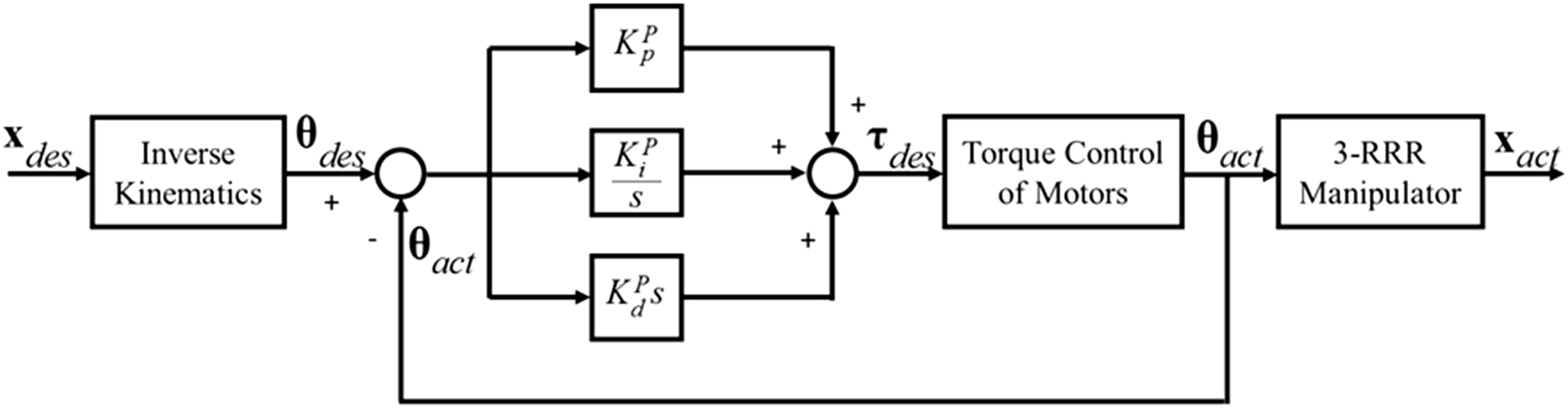
The CTC regulates the angular accelerations of the motors, so good tracking performances on the motor angles can be expected. To eliminate the nonlinear terms in equation (18), the control torque $τ$ can be designed as³⁶

τ = M (θ_{act}) {\ddot{θ}}_{ref} + C (θ_{act}, {\dot{θ}}_{act}) + H (θ_{act}) + B ({\dot{θ}}_{act})

(23)

where

{\ddot{θ}}_{ref}

is a vector of reference angular accelerations, and each acceleration component is defined as

{\ddot{θ}}_{ref} = {\ddot{θ}}_{des} + K_{p}^{C} e_{θ} + K_{d}^{C} {\ddot{e}}_{θ}

(24)

where

K_{p}^{C}

and

K_{d}^{C}

are the controller gains. Substituting equations (23) and (24) into equation (18) leads to an error dynamics with the CTC as

{\ddot{e}}_{θ} + K_{d}^{C} {\dot{e}}_{θ} + K_{p}^{C} e_{θ} = 0

(25)

where the controller gains can be designed to obtain a desired error response.

Figure 4 shows the block diagram of the CTC. Referring to this diagram, the desired trajectory of the end-effector is generated first, and the reference angular accelerations are obtained by using a PD controller plus the desired angular accelerations. Besides, the inverse dynamics is used to calculate the control torques applied to the manipulator. Since the control scheme uses the motor angles as feedback control signals instead of the position and orientation angle of the end-effector as them, encoders are the only sensors used in this control scheme. It is worth to note that the CTC needs the angular rates of the active angles, and they are calculated by applying a finite difference method to the active angles. In Figure 4, the symbol s represents the differentiation with respect to time and s² refers to the double differentiation.

Figure 4.

Block diagram of the CTC scheme.

Resolved acceleration control

In contrast to the CTC, the RAC regulates the position and the orientation angle of the end-effector, so the control scheme can provide better control tracking performances on them. To develop the RAC, the control torque $τ$ is the same as equation (23), and then the equation substituted into the dynamics in equation (18) leads to

\ddot{θ} = {\ddot{θ}}_{ref}

(26)

Applying the acceleration inversion in equation (6) into equation (26) yields

\ddot{x} = {\ddot{x}}_{ref}

(27)

where

{\ddot{x}}_{ref}

is the reference acceleration defined as

{\ddot{x}}_{ref} = {\ddot{x}}_{des} + K_{p}^{R} e_{x} + K_{d}^{R} {\dot{e}}_{x}

(28)

in which

K_{p}^{R}

and

K_{d}^{R}

are the controller gains, and the error

e_{x}

is defined as

e_{x} = x_{des} - x_{act}

(29)

To ensure the stability, equation (28) substituted into equation (27) leads to

{\ddot{e}}_{x} + K_{d}^{R} {\dot{e}}_{x} + K_{p}^{R} e_{x} = 0

(30)

where the controller gains

K_{p}^{R}

and

K_{d}^{R}

can be designed to obtain a desired error response.

Figure 5 shows the block diagram of the RAC applied to a manipulator. Referring to the figure, the desired trajectory of the end-effector is generated first based on trajectory planning, and then the reference trajectory is calculated based on a PD controller plus the desired acceleration. Besides, the reference angular accelerations are calculated by applying the inverse dynamics. Since the only sensors are used in the control scheme are encoders, it is necessary to have the actual position and orientation angle of the end-effector by using the direct kinematics and the velocity inversion, which will be feedback control signals in the control scheme.

Figure 5.

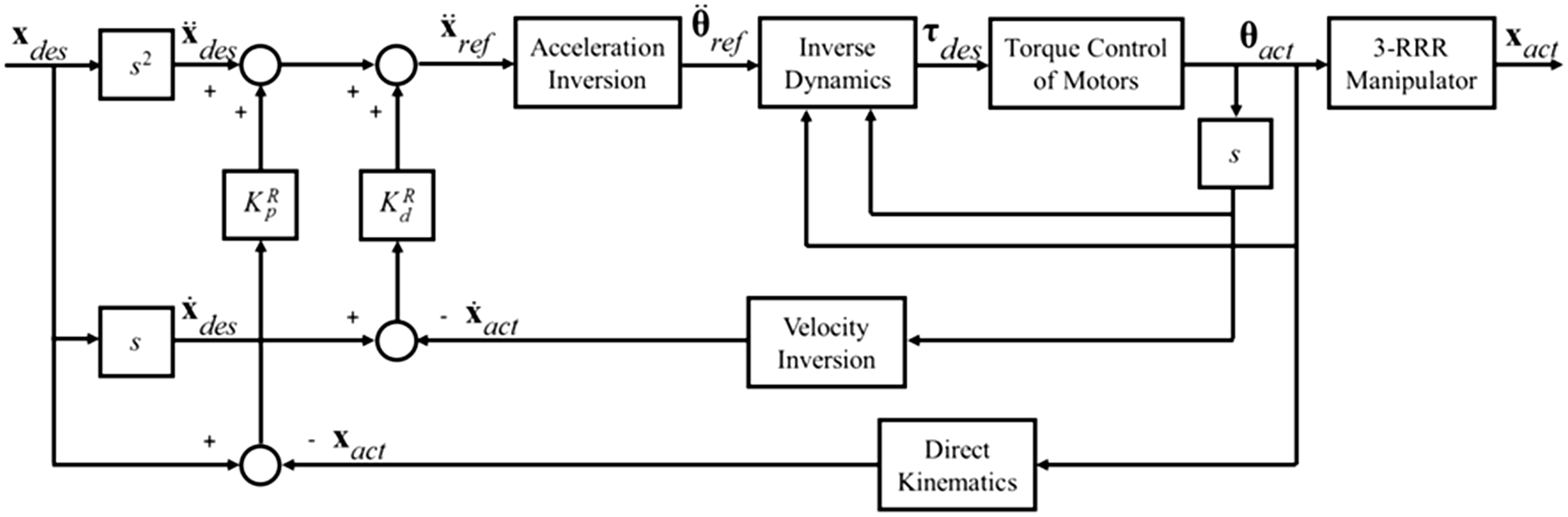
Block diagram of the RAC scheme.

Visual servoing resolved acceleration control

This paper proposes a VSRAC scheme, which can be treated as an extended RAC. Since the RAC regulates the linear and angular accelerations of the end-effector, it is necessary to have its positions and velocities, which can be obtained through direct kinematics and velocity inversion by using the motor angles. There are two major disadvantages in this control scheme. One is that the computational cost increased, and the other one direct kinematics and velocity inversion may not provide accurate position and velocity of the end-effector. To improve the two disadvantages, a camera and image processing techniques are utilized directly to obtain the position and the orientation angle of then-effector.

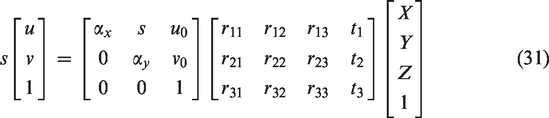
Figure 6 shows the block diagram of the proposed control scheme. The block diagram is similar as one of the RAC except for the direct kinematics and the velocity inversion replaced by a camera and image processing, whose purpose is to acquire the position of the end-effector. Thus, it is necessary to have a camera model, which will be used to calculate the position in three-dimensional space. The relationship between an image frame coordinate system and a global coordinate system as

s [\begin{matrix} u \\ v \\ 1 \end{matrix}] = [\begin{matrix} α_{x} & s & u_{0} \\ 0 & α_{y} & v_{0} \\ 0 & 0 & 1 \end{matrix}] [\begin{matrix} r_{11} & r_{12} & r_{13} & t_{1} \\ r_{21} & r_{22} & r_{23} & t_{2} \\ r_{31} & r_{32} & r_{33} & t_{3} \end{matrix}] [\begin{matrix} X \\ Y \\ Z \\ 1 \end{matrix}]

(31)

where (u, v) are the frame coordinates; (X, Y, Z) are the global coordinates;

t_{i}

and

r_{ij}

are the translation and rotation parameters, which are called the extrinsic parameters of camera;

α_{x}

α_{y}

u_{0}

, and

v_{0}

are the pixel values of the focus at the u-direction, the focus at the v-direction, the origin at the u-direction, the origin at the v-direction, respectively, which are called the intrinsic parameters of camera;

s

is the skew parameter.

Figure 6.

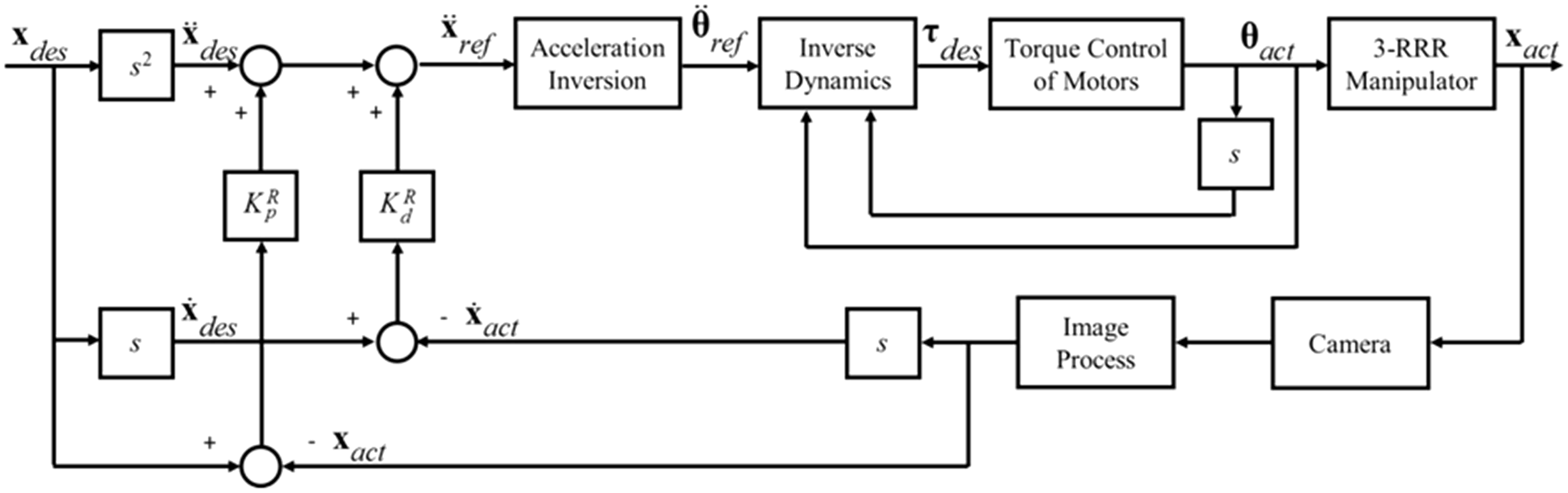
Schematic diagram of the VBRAC scheme.

After capturing the image of the manipulator by a camera, the position of the orientation angle of the end-effector can be obtained by using equation (31), and the velocity can be further calculated through the difference method.

Experimental setup

This section introduces the experimental setup, which will be divided into two subsections, the manipulator and the control system.

The manipulator

The manipulator is shown in Figure 7(a), where the central part (the triangle) is the end-effector, and there are three kinematic chains connect it with the motors, which are fixed on the platform and can be seen in Figure 7(b). Besides, each kinematic chain consists of two links, which are connected by revolute joints.

Figure 7.

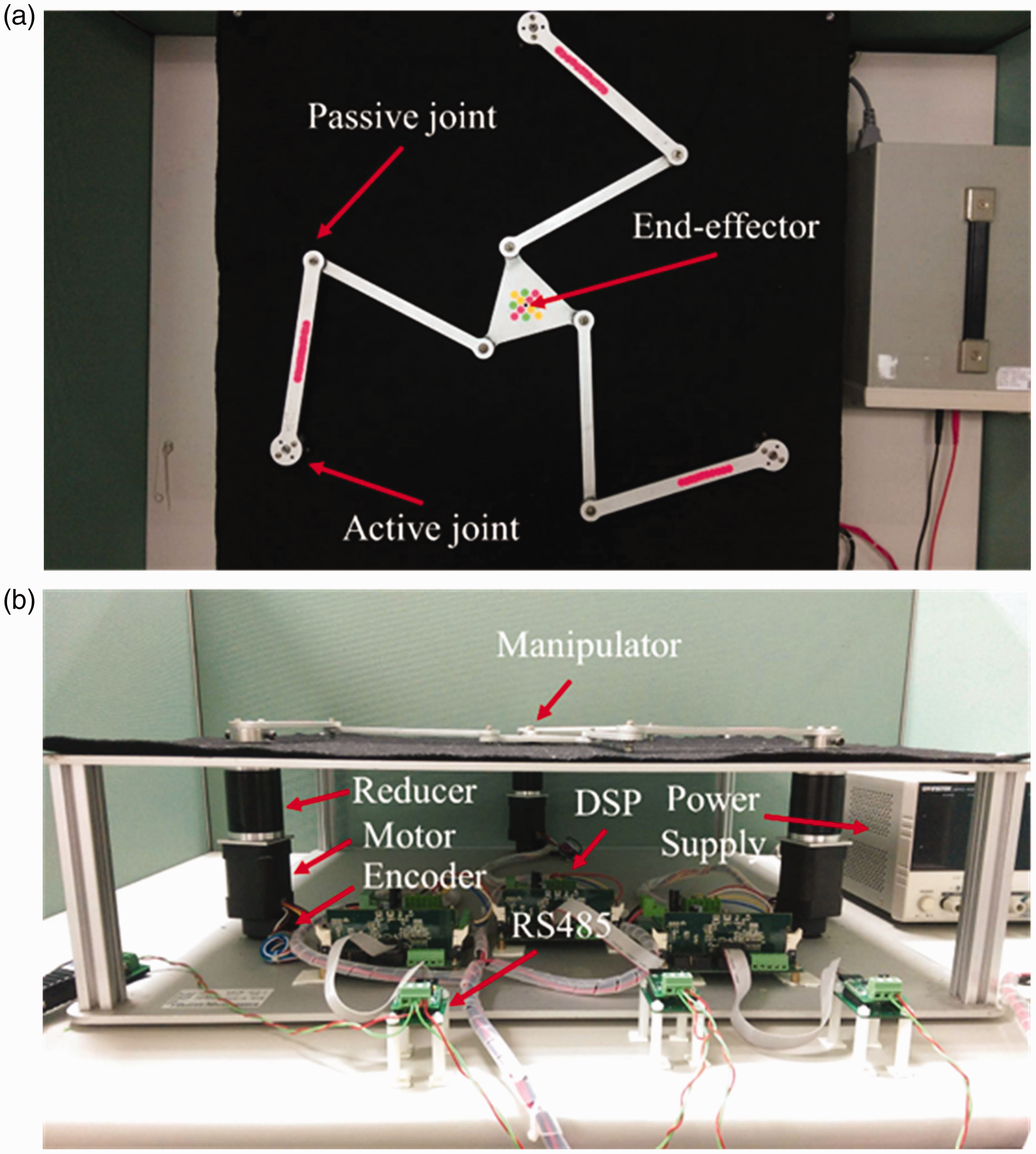
The prototype of the planar 3-DOF parallel manipulator, (a) a top view and (b) a side view. DSP: digital signal processing.

Control system

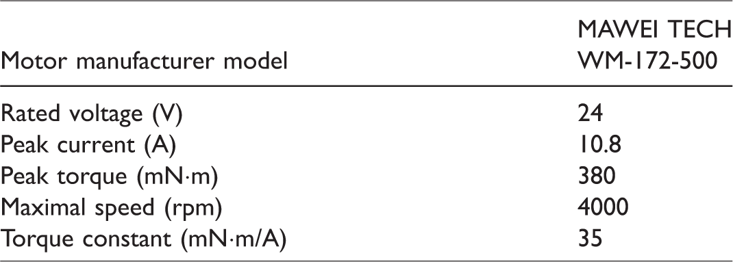
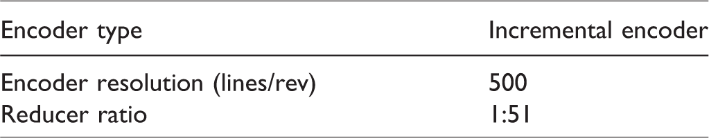
Since this study emphasizes the torque-based control schemes, there is an inner current control loop to facilitate the torque control for each motor. Besides, the motor torque is proportional to the electrical current of the motor, so a desired torque is divided by a torque constant so as to obtain a desired electrical current. The block diagram is shown in Figure 2, where a current sensor is used to sense the motor current and then the signal is fed back to a PID controller, which is embedded in a digital signal processing (DSP). The current sensor uses a resistance with 0.01 Ω, and the sensing precision is ±1%. The manipulator is driven by using three three-phase DC brushless motors, and the motor specifications are listed on Table 1. Three encoders are used to sense the rotating angles of the three motors, and the encoder specifications are listed on Table 2. Based on this table, the accuracy of the encoder is 0.0141°. The entire control block diagrams for the three control schemes have been introduced in “Torque-based control schemes” section. The controller of the manipulator is programmed and stored in a personal computer (PC). The specifications of the DSP and the PC are listed in Table 3, and the calculation functions of both are arranged in Table 4. The entire hardware-in-the-loop diagram is illustrated in Figure 8. The programming language is used in C language.

Table 1.

Motor specifications.

Motor manufacturer model	MAWEI TECH WM-172-500
Rated voltage (V)	24
Peak current (A)	10.8
Peak torque (mN·m)	380
Maximal speed (rpm)	4000
Torque constant (mN·m/A)	35

Table 2.

Encoder specifications.

Encoder type	Incremental encoder
Encoder resolution (lines/rev)	500
Reducer ratio	1:51

Table 3.

Specifications of the PC and DSP.

	PC	DSP
OS	Windows 7 (x64)	–
CPU	Intel Core i5 (3.2 GHz)	TMS320F28335 (150 MHz)
RAM	8 GB	68 KB

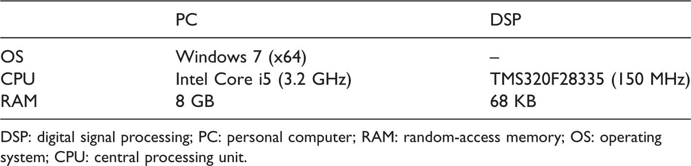
DSP: digital signal processing; PC: personal computer; RAM: random-access memory; OS: operating system; CPU: central processing unit.

Table 4.

Calculation functions of the PC and DSP.

	PC	DSP
Calculation functions	1. Direct and inverse Kinematics 2. Inverse dynamics3. Controller for the implementations of PID, RAC, and CTC4. Image Processing	1. Controller for current control 2. Generate PWM signal

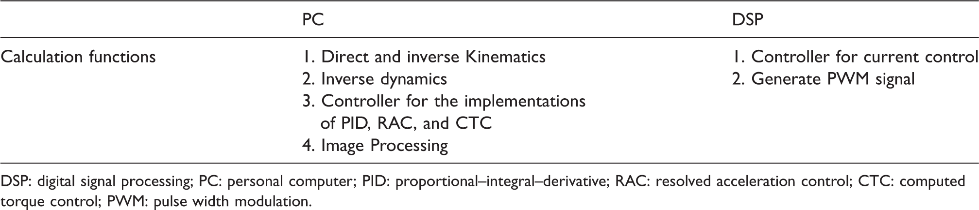
DSP: digital signal processing; PC: personal computer; PID: proportional–integral–derivative; RAC: resolved acceleration control; CTC: computed torque control; PWM: pulse width modulation.

Figure 8.

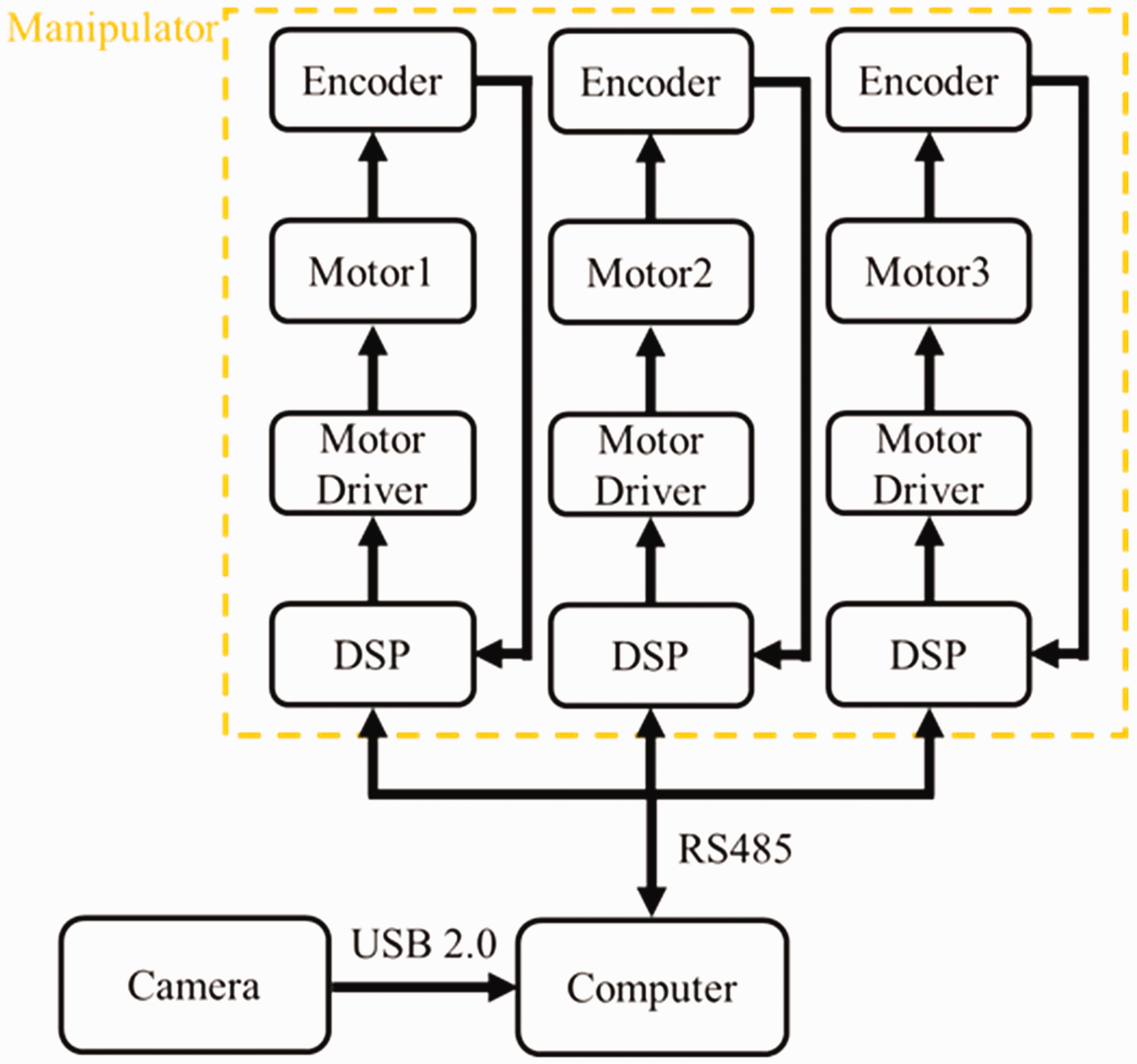
Hardware-in-the-loop diagram. DSP: digital signal processing.

Visual system

The experimental setup is shown in Figure 9, which includes the manipulator and a camera. The camera is mounted right above the manipulator in order to capture the entire image of the manipulator, so the distance between them is set as 81 cm. The camera is made by Logitech Ltd., and the camera type is HD Webcam C615. The resolution is 1920 × 1080, and the maximum frame rate is 60 Hz.

Figure 9.

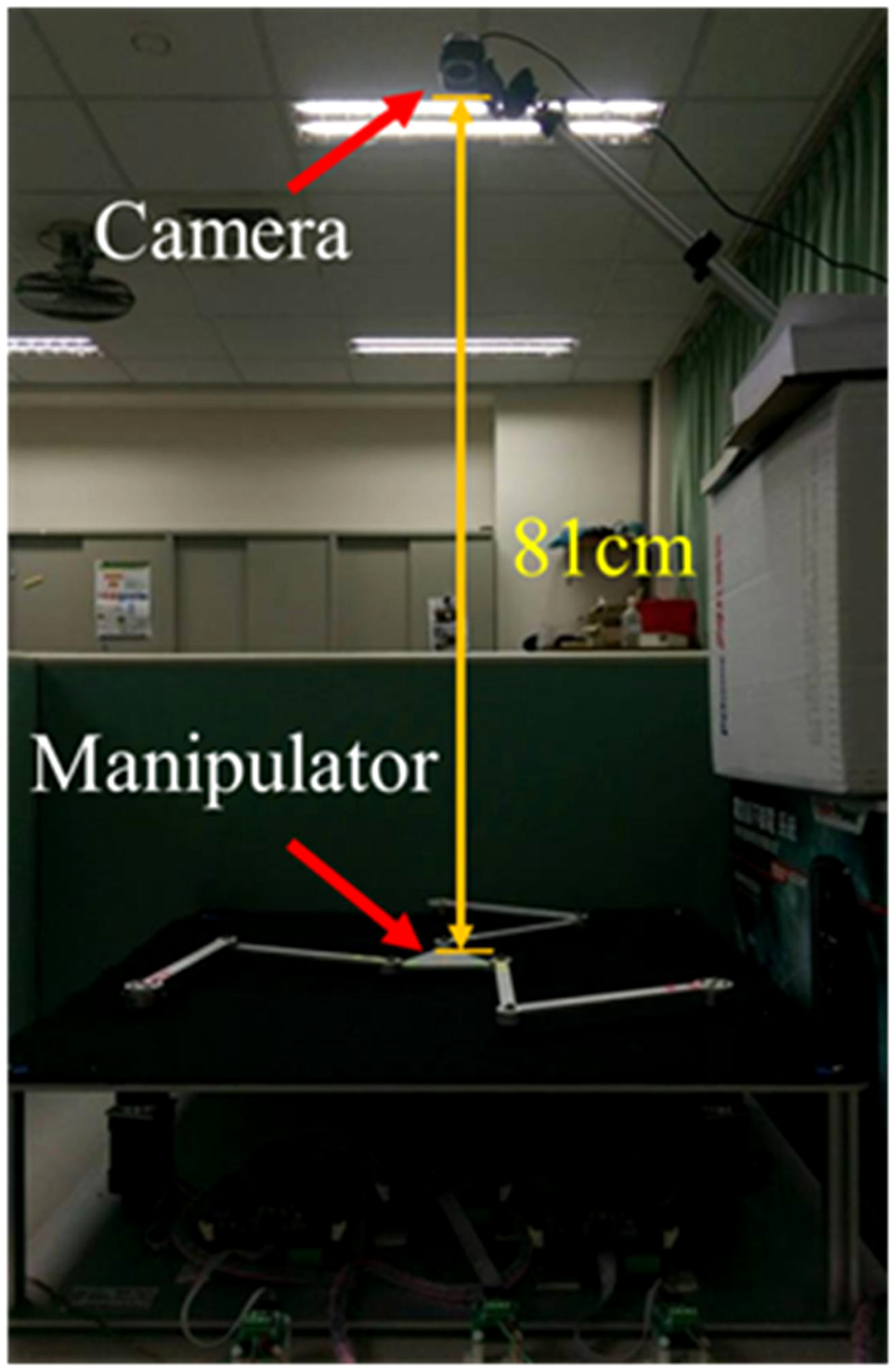
Experimental setup of the 3-DOF planar parallel manipulator and the camera.

Graphical user interface

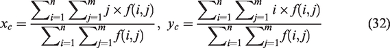
This study also develops a graphical user interface which shows the image of the manipulator and the positions of the end-effector and the active and passive links in real time, where the positions are obtained by using some image processing techniques, and the interface is developed by using C language. Figure 10 shows the procedure of performing some image processing techniques to identify a feature point on an image, where the feature point refers to a small red round sticker attached on the center of the end-effector of the manipulator. There are four steps in this procedure. The first one is to obtain the image of the entire manipulator by using a CCD. The second step is to identify the feature point. The third step is erosion, which eliminates noises of background image. The last step is dilation, which forms a fully solid circle. To locate the coordinate of the feature point, the formulas of the center of area is utilized and shown as

x_{c} = \frac{\sum_{i = 1}^{n} \sum_{j = 1}^{m} j \times f (i, j)}{\sum_{i = 1}^{n} \sum_{j = 1}^{m} f (i, j)}, y_{c} = \frac{\sum_{i = 1}^{n} \sum_{j = 1}^{m} i \times f (i, j)}{\sum_{i = 1}^{n} \sum_{j = 1}^{m} f (i, j)}

(32)

where

(x_{c}, y_{c})

is the coordinates of the center of area;

n

and

m

are the numbers of pixels in two dimensions;

f (i, j)

is the pixel value of point

(i, j)

; the denominator represents the area of the feature point.

Figure 10.

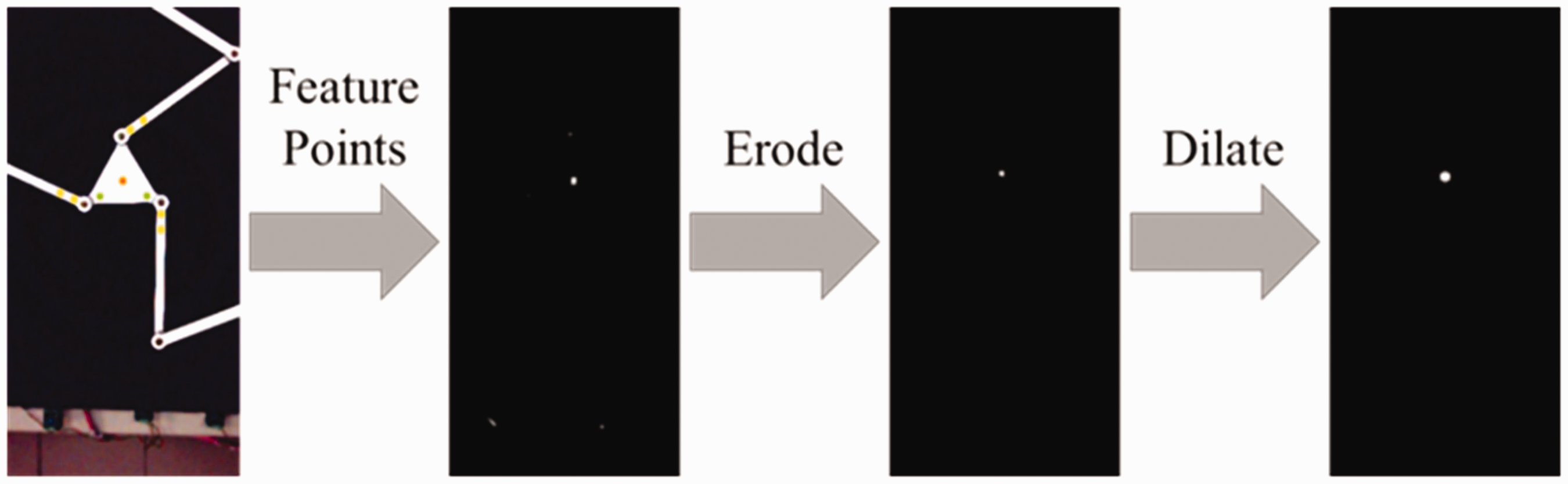
Feature point capture process.

Based on the aforementioned procedure to determine the coordinate of a feature point, the other points can be located to determine the origin, the coordinate systems, and the points on the active and passive links shown in Figure 11, and then the vectors representing the active and passive link can be obtained. Furthermore, the rotating angles of the active and passive links can be determined through vector operation. Figure 12 shows the developed graphical user interface, which includes the image of the entire manipulator, the results by performing image processing, and the positions and the angles of all components of the manipulator.

Figure 11.

Identification of feature points on the manipulator.

Figure 12.

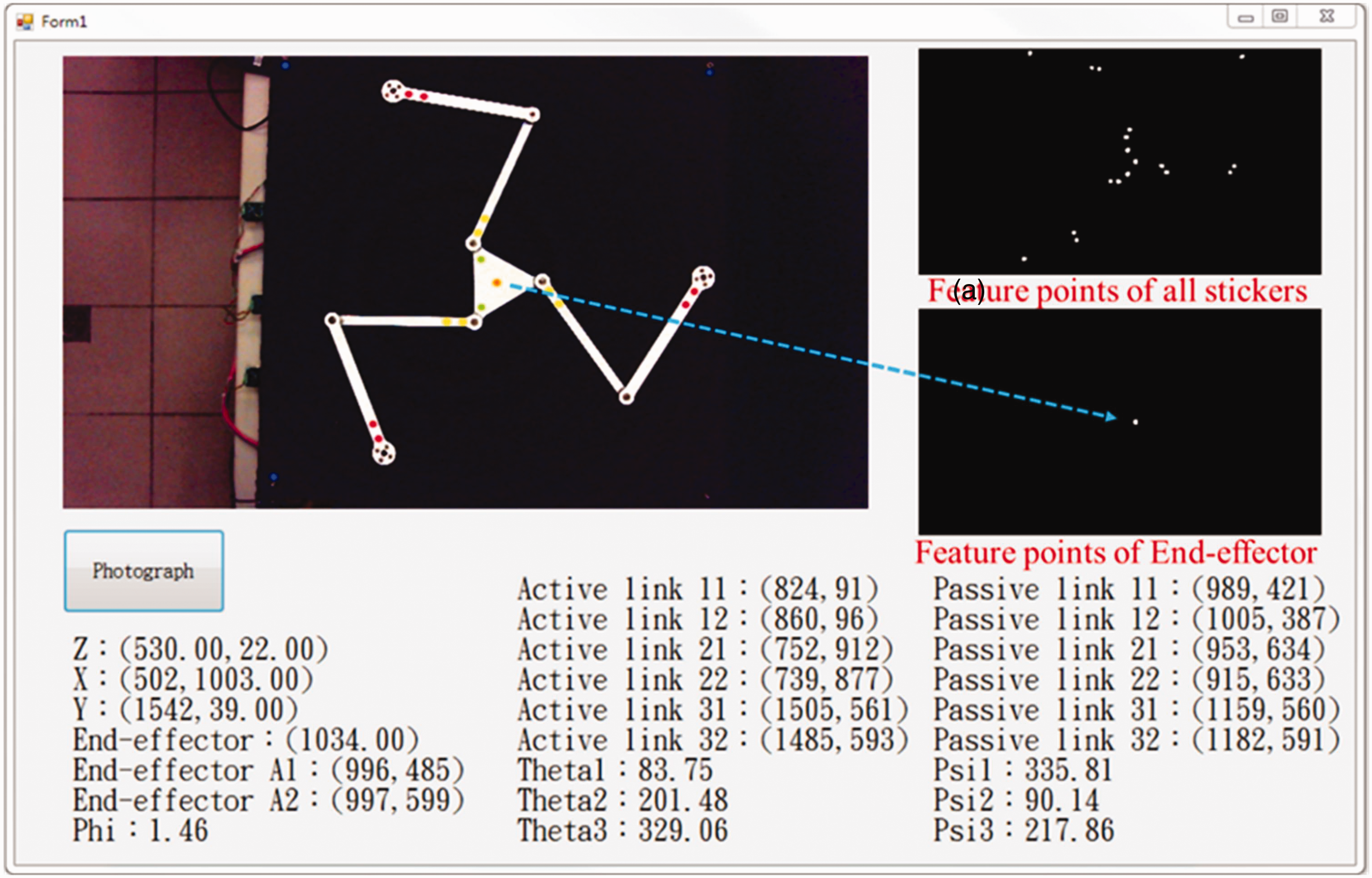
Image processing interface.

Simulation and experimental results

This section presents the simulation and experimental procedures, the system and control parameters, and the simulation and experimental results by exploring four controllers shown in “Torque-based control schemes” section.

Simulation and experimental procedure

The experimental process is the first to design the trajectory. The desired trajectory of the end-effector is defined as

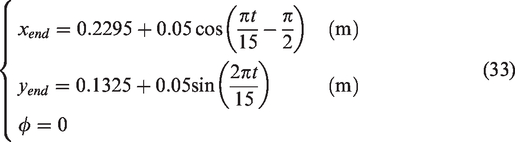
{\begin{array}{l} x_{end} = 0.2295 + 0.05 \cos (\frac{π t}{15} - \frac{π}{2}) (m) \\ y_{end} = 0.1325 + 0.05 \sin (\frac{2 π t}{15}) (m) \\ ϕ = 0 \end{array}

(33)

Thus, the x- and y-directional translation motions of the end-effector are, respectively, kept within $0.2295 \pm 0.05$ and $0.1325 \pm 0.05$ m, and the orientation angle of the end-effector is always kept as 0°. The motion time of the manipulator is from 0 to 30 s. Figure 13 illustrates the procedure of calculating the control torques for the four control schemes. The PID control uses the errors of the motor angles to calculate the control torques. The CTC uses both errors of the motor angles and angular rates to calculate the control torques. The RAC uses the reference accelerations of the end-effector to calculate the control torques. The VSRAC is similar as the RAC except for the direct kinematics and the velocity inversion replaced by a camera and image processing. For each control scheme, the calculated control torques are delivered to the motors through DSP. Figure 14 illustrates the flow chart of programming codes. The simulation procedure is similar as the experimental procedure except for the motors replaced by the motor models, and the simulations are performed by using the software Matlab.

Figure 13.

Flow charts of the control experiments. PID: proportional–integral–derivative; RAC: resolved acceleration control; CTC: computed torque control; VSRAC: visual servoing resolved acceleration control scheme.

Figure 14.

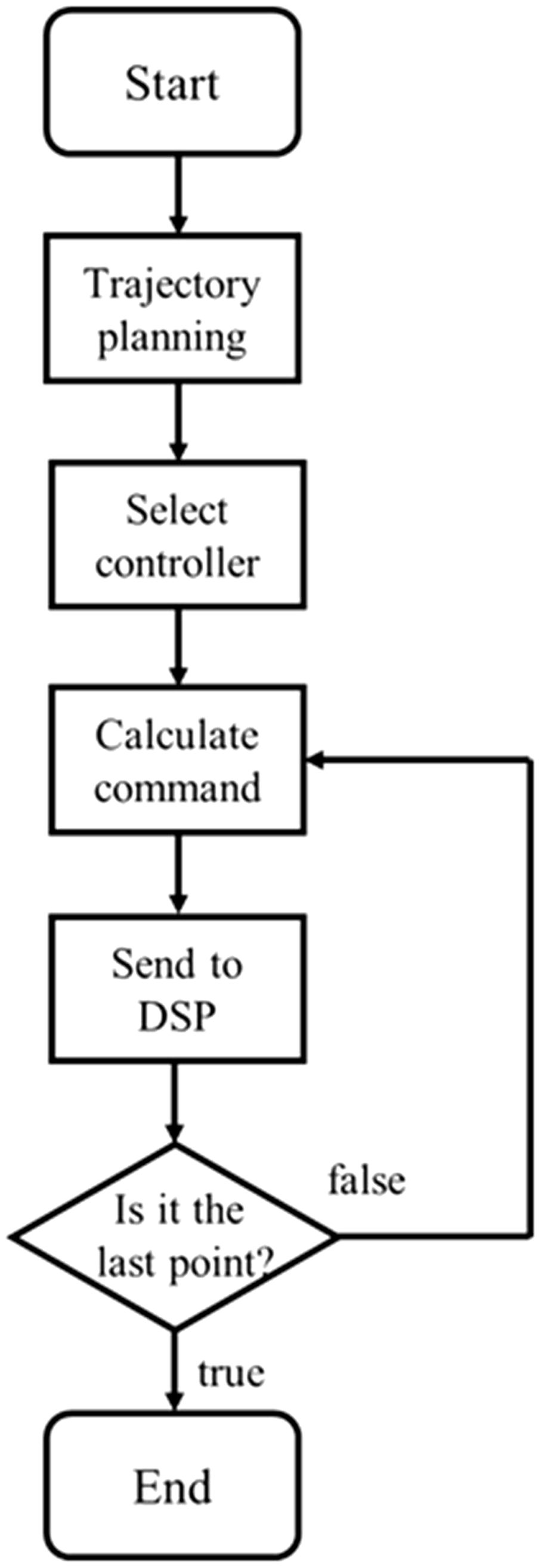
Flow chart of program codes. DSP: digital signal processing.

System and controller parameters

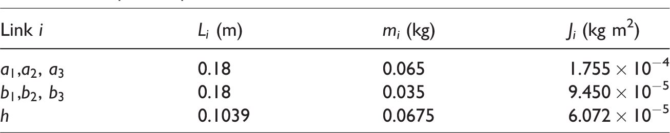
The link parameters of the manipulators are listed in Table 5, and the end-effector is an equilateral triangle with 0.1039 m side length and active angles are separated by 0.459 m from each other. Based on the models and the control schemes, respectively, presented in “A 3-DOF planar parallel manipulator” and “Torque-based control schemes” sections, one uses the software Matlab to perform numerical simulations in order to obtain the controller gains listed in Table 6, where the gain $K_{i}$ of the PID control is zero due to a PD controller applied. Besides, the controller gains will be used in the following experiments. For the VSRAC scheme, it is necessary to have the parameters of the camera model shown in equation (31). One user performs a calibration experiment first for the camera, and then the software Matlab Camera Calibration Toolbox is used to calculate the parameters of the camera model, so the parameters are obtained as listed in Tables 7 and 8 for the intrinsic and extrinsic parameters, respectively. Based on the camera model, one performs an experiment to test the accuracy, and the errors of the x- and y-axes are 3% and 1%, respectively.

Table 5.

Manipulator parameters.

Link $i$	$L_{i}$ (m)	m_i (kg)	J_i (kg m²)
$a_{1}$ , $a_{2}$ , $a_{3}$	0.18	0.065	1.755 × 10⁻⁴
$b_{1}$ , $b_{2}$ , $b_{3}$	0.18	0.035	9.450 × 10⁻⁵
$h$	0.1039	0.0675	6.072 × 10⁻⁵

Table 6.

Controller gains.

Controller parameters	PID	CTC	RAC	VSRAC
$K_{p}$	1	10	10	10
$K_{i}$	0	0	0	0
$K_{d}$	0.05	0.5	0.5	0.5

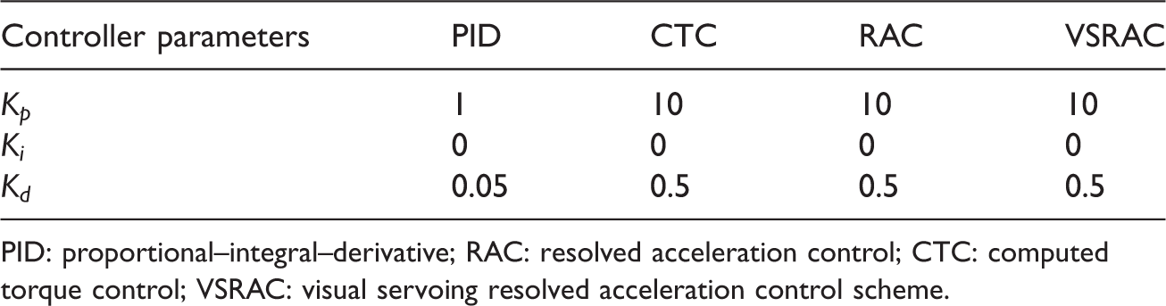
PID: proportional–integral–derivative; RAC: resolved acceleration control; CTC: computed torque control; VSRAC: visual servoing resolved acceleration control scheme.

Table 7.

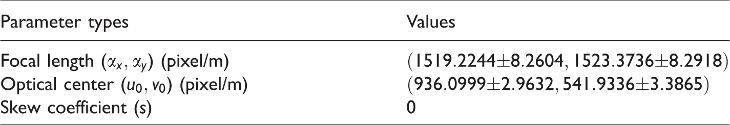
Intrinsic parameters of the camera model.

Parameter types	Values
Focal length ( $α_{x}, α_{y}$ ) (pixel/m)	$(1519.2244 \pm 8.2604, 1523.3736 \pm 8.2918)$
Optical center ( $u_{0}, v_{0}$ ) (pixel/m)	$(936.0999 \pm 2.9632, 541.9336 \pm 3.3865)$
Skew coefficient ( $s$ )	0

Table 8.

Extrinsic parameters of the camera model.

Parameter types	Values
Rotation matrix $[\begin{matrix} r_{11} & r_{12} & r_{13} \\ r_{21} & r_{22} & r_{23} \\ r_{31} & r_{32} & r_{33} \end{matrix}]$	$[\begin{matrix} 0.9998 & 0.0134 & - 0.0143 \\ - 0.0139 & 0.9993 & - 0.0354 \\ 0.0138 & 0.0356 & 0.9993 \end{matrix}]$
Translation matrix $[\begin{matrix} T_{11} \\ T_{21} \\ T_{31} \end{matrix}]$	$[\begin{matrix} - 226.8314 \\ - 166.0977 \\ 830.2091 \end{matrix}]$

Simulation results

This subsection presents the simulation results by using only the three control schemes except for the VSRAC, because it needs images captured by a camera. Figure 15 shows the results using the PID control, where Figure 15(a) shows the trajectories of the command and the simulation results for the end-effector of the manipulator and Figure 15(b) shows the trajectory error as a function of time. The results show that both the trajectories of the command and the simulation results are very close in Figure 15(a). However, by examining the error, it indicates the error reaches 1.3 × 10⁻³ m in the beginning, but it reduces as 1.0 × 10⁻⁴ m after that. Figure 16 shows the results using the CTC control, where Figure 16(a) shows the trajectories of the command and the simulation results for the end-effector of the manipulator, and Figure 16(b) shows the trajectory error as a function of time. The results show that both the trajectories of the command and the simulation results are slightly different in Figure 16(a), and the error response is oscillating and decaying as time increases. The error reduces around from 7 × 10⁻³ to 2 × 10⁻³ m. Figure 17 shows the results using the RAC control, where Figure 17(a) shows the trajectories of the command and the simulation results for the end-effector of the manipulator and Figure 17(b) shows the trajectory error as a function of time. The results show that both the trajectories of the command and the simulation results are slightly different in Figure 17(a), and the error response is oscillating and decaying as time increases. The error reduces around from 7 × 10⁻³ to 2 × 10⁻³ m. To compare the results, Table 9 lists the errors by using the three control schemes, where the error of the trajectory is defined as

e_{end} = \sqrt{{(x_{end, des} - x_{end, act})}^{2} + {(y_{end, des} - y_{end, act})}^{2}}

(34)

where subscript des and act refer to the desired and actual trajectories. And, the results show that the PID control provides better tracking accuracy of the end-effector, and the accuracies of the CTC and RAC are close.

Figure 15.

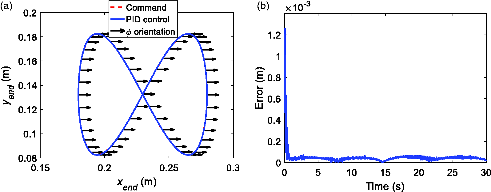
Simulation results of the end-effector trajectory by using the PID scheme: (a) the moving trajectory and (b) the error response. PID: proportional–integral–derivative.

Figure 16.

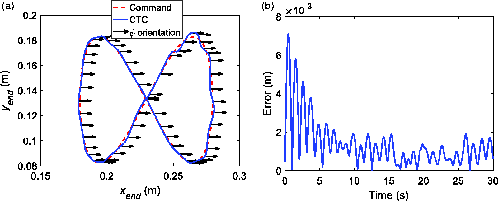
Simulation results of the end-effector by using the CTC scheme: (a) the moving trajectory and (b) the error response. CTC: computed torque control.

Figure 17.

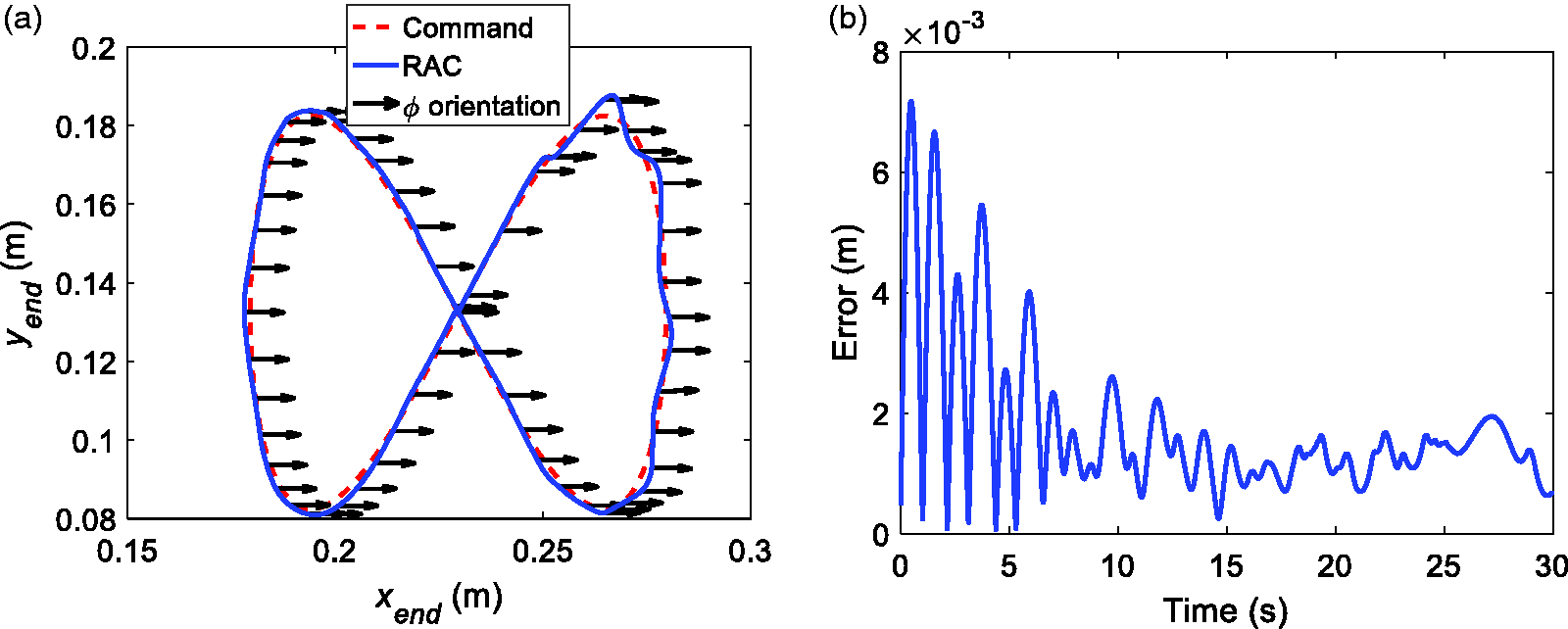
Simulation results of the end-effector by using the RAC scheme: (a) the moving trajectory and (b) the error response. RAC: resolved acceleration control.

Table 9.

RMS errors of the simulation results.

RMS^	PID	CTC	RAC
$θ_{1}$ (deg)	0.064	0.432	0.426
$θ_{2}$ (deg)	0.104	0.636	0.787
$θ_{3}$ (deg)	0.074	0.551	0.607
$x_{end}$ (m)	3.682 × 10⁻⁵	9.249 × 10⁻⁴	9.044 × 10⁻⁴
$y_{end}$ (m)	7.715 × 10⁻³	1.557 × 10⁻³	1.933 × 10⁻³
$ϕ$ (deg)	0.018	0.910	0.866
Trajectory (m)	8.549 × 10⁻⁵	1.811 × 10⁻³	2.134 × 10⁻³

PID: proportional–integral–derivative; RAC: resolved acceleration control; CTC: computed torque control; RMS: root mean square.

Experimental results

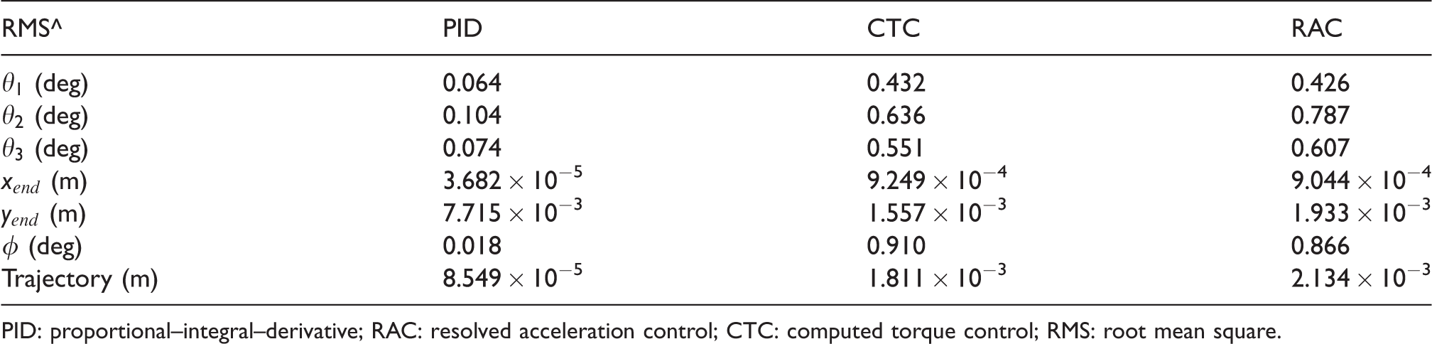
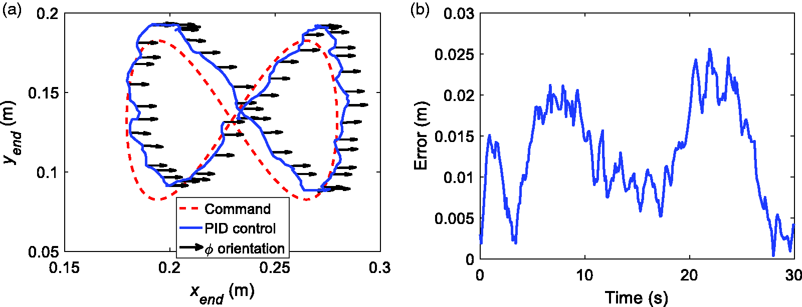
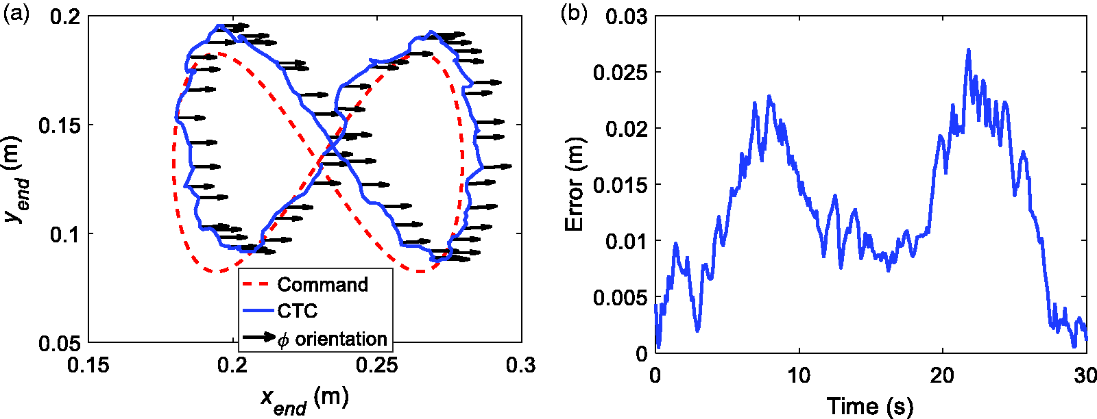
This subsection presents the experimental results by using the proposed VSRAC and the results are compared with those by using the other three control schemes. Figure 18 shows the results using the PID control, where Figure 18(a) shows the trajectories of the command and the experimental results for the end-effector of the manipulator and Figure 18(b) shows the trajectory error as a function of time. The results show that both the trajectories of the command and the experimental results are not exactly consistent in Figure 18(a), and the maximum error range is around 0.025 m during the moving period. Figure 19 shows the results using the CTC scheme, where Figure 19(a) shows the trajectories of the command and the experimental results for the end-effector of the manipulator and Figure 19(b) shows the trajectory error as a function of time. The results show that both the trajectories of the command and the experimental results are not exactly consistent in Figure 19(a), and the maximum error is around 0.025 m during the moving period. The results are similar to those by using the PID control. Figure 20 shows the results using the RAC scheme, where Figure 20(a) shows the trajectories of the command and the experimental results for the end-effector of the manipulator and Figure 20(b) shows the trajectory error as a function of time. The results show that both the trajectories of the command and the experimental results are not exactly consistent in Figure 20(a), and the maximum error is around 0.020 m during the moving period. The errors are little smaller than those by using the PID and CTC schemes. Figure 21 shows the results using the proposed VSRAC scheme, where Figure 21(a) shows the trajectories of the command and the experimental results for the end-effector of the manipulator, and Figure 21(b) shows the trajectory error as a function of time. The results show that both the trajectories of the command and the experimental results are exactly consistent in Figure 21(a), and the maximum error is around 0.017 m during the moving period. The error is much smaller than those by using the other schemes.

Figure 18.

Experimental results of the end-effector by using the PID control: (a) moving trajectory and (b) error response. PID: proportional–integral–derivative.

Figure 19.

Experimental results of the end-effector by using the CTC scheme: (a) the moving trajectory and (b) the error response. CTC: computed torque control.

Figure 20.

Experimental results of the end-effector by using the RAC scheme: (a) the moving trajectory and (b) the error response. RAC: resolved acceleration control.

Figure 21.

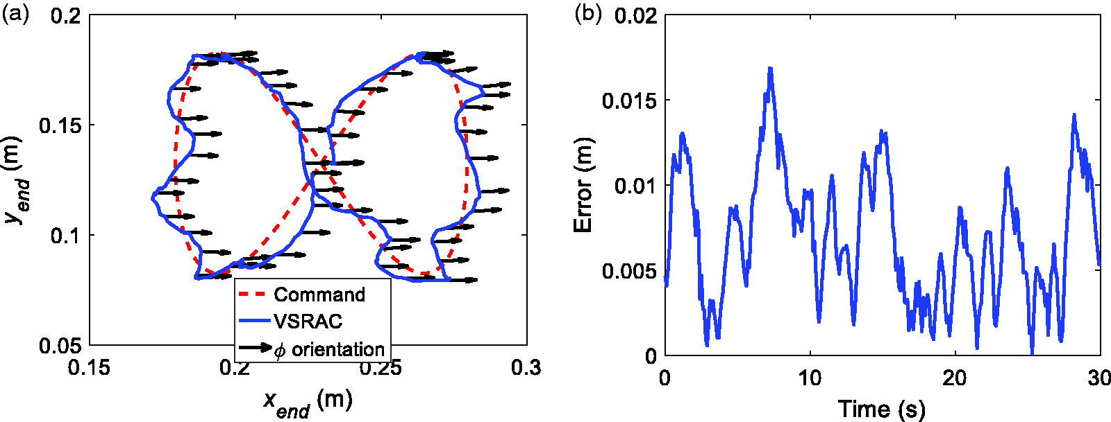
Experimental results of the end-effector by using the VSRAC scheme: (a) the moving trajectory and (b) the error response. VSRAC: visual servoing resolved acceleration control scheme.

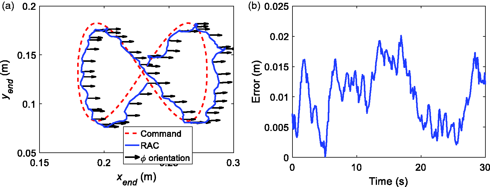
To compare the four schemes, Table 10 lists several root mean square (RMS) errors, where the errors of the active angles θ_i are the differences between the command signals and the encoder values, and the errors of the end-effector are the differences between the command signals and the values through image processing. The results show that the proposed VSRAC provides the smallest errors on the trajectory tracking of the end-effector. The CTC scheme is better than the RAC scheme on the tracking of motor angles, because the CTC regulates the angular accelerations of the motor angles. Besides, the PID control does not need the manipulator dynamics, which causes the largest tracking error to compare with the other three schemes. To compare the simulation and experimental results, it is obvious to note that the tracking performances of the experiments are worse than those of the simulations, because there are some factors affecting the tracking performances, such as the manufacturing inaccuracy of the experimental platform, the motor accuracy due to the backlashes, and the accuracy of the encoders and the current sensors, and the capabilities of the DSP dealing the calculations and data transmissions. To further investigate the four schemes, Table 11 lists their required calculation tasks and the computation time. The results show that the PID control does not carry out the calculations of the inverse dynamics, which causes the less computation time. The RAC scheme needs the most tasks on the calculations, so it needs the most computation time. The CTC needs to calculate the inverse dynamics and the inverse kinematics, so its computation time is less that of the RAC scheme. The proposed VSRAC uses a camera and some image processing techniques to directly obtain the position and the orientation angle of the end-effector instead of using the velocity and acceleration inversions. Thus, this reduces computation time to compare with the RAC scheme, and the more accurate positions and the orientation angle of the end-effector can be obtained. Based on the hardware specifications used in the VSRAC experiments, the sampling frequencies of the inner and outer loops are 10 and 60 Hz.

Table 10.

RMS errors of the experiments.

RMS	PID	CTC	RAC	VSRAC
$θ_{1}$ (deg)	1.171	0.825	1.201	2.583
$θ_{2}$ (deg)	1.675	1.354	1.803	3.085
$θ_{3}$ (deg)	1.296	0.808	0.867	2.544
$x_{end}$ (m)	5.49 × 10⁻³	5.936 × 10⁻³	7.281 × 10⁻³	4.497 × 10⁻³
$y_{end}$ (m)	1.311 × 10⁻²	1.266 × 10⁻²	8.635 × 10⁻³	6.487 × 10⁻³
$ϕ$ (deg)	2.123	2.149	2.437	4.214
Trajectory (m)	1.422 × 10⁻²	1.398 × 10⁻²	1.13 × 10⁻²	7.894 × 10⁻³

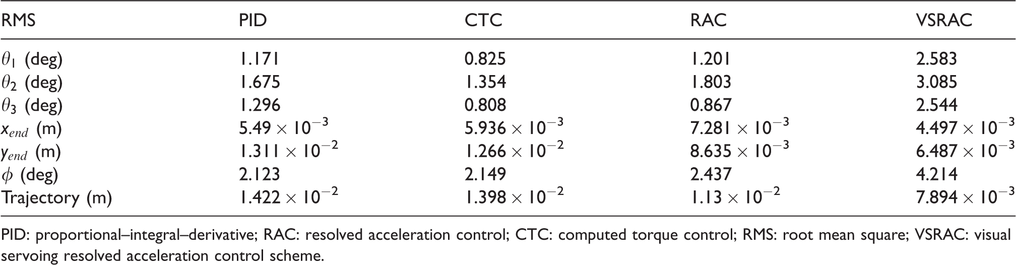
PID: proportional–integral–derivative; RAC: resolved acceleration control; CTC: computed torque control; RMS: root mean square; VSRAC: visual servoing resolved acceleration control scheme.

Table 11.

Comparisons of control schemes.

Controller	PID	CTC	RAC	VSRAC
Required calculation tasks	• Inverse kinematic	• Inverse kinematics • Inverse dynamic	• Direct kinematics• Inverse dynamics• Velocity inversion• Acceleration inversion	• Image processing• Inverse dynamics• Acceleration inversion
Computation time (ms)	0.358	42.606	44.148	42.656

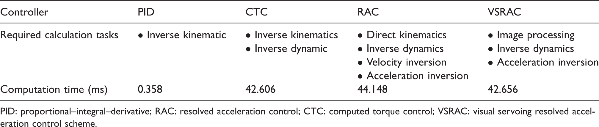
PID: proportional–integral–derivative; RAC: resolved acceleration control; CTC: computed torque control; VSRAC: visual servoing resolved acceleration control scheme.

Conclusions

This paper presents a VSRAC scheme, which regulates the accelerations of the position and the orientation angle of the end-effector by imposing a visual servo approach. Besides, this scheme is applied to a 3-DOF planar parallel manipulator, and the control performances are compared with those by applying three existing schemes. To compare with the RAC scheme, the proposed scheme utilizes a camera and some image processing techniques to directly obtain the position and the orientation angle of the end-effector instead of calculating the direct kinematics and the velocity inversion, so the computation time is reduced. Besides, directly having the position and the orientation angle through image processing can acquire more accurate values than an indirect approach by the direct kinematics, because there might be some errors caused by the motors and the manipulator mechanism. Furthermore, due to the derivation complexity of the dynamic models of parallel manipulators, an approach is proposed by imposing the Jacobian matrices relating the passive and active links into the Euler-Lagrange’s equation. Both numerical simulation and experimental validations are performed for the proposed scheme applied to the manipulator. The experimental results show that the tracking errors of the end-effector are smaller than those by applying other schemes, and the computation time is smaller than that by applying the RAC scheme.

Footnotes

Declaration of conflicting interests

The author(s) declared no potential conflicts of interest with respect to the research, authorship, and/or publication of this article.

Funding

The author(s) disclosed receipt of the following financial support for the research, authorship, and/or publication of this article: This study was supported in part by the Ministry of Science and Technology, Taiwan, under Grant MOST 106‐2221‐E‐011‐085.

References

Gosselin

Angeles

The optimum kinematic design of a planar three-degree-of-freedom parallel manipulator. J Mech Trans 1988; 110: 35–41.

Lee

Yien

Design and control of a prototype platform manipulator for workholding and workhandling applications. J Mech Work Technol 1989; 20: 305–314.

Gosselin

Sefrioui

Polynomial solutions for the direct kinematic problem of planar three-degree-of freedom parallel manipulators. In: IEEE international conference on advanced robotics, Pisa, Italy, pp. 1124–1129. Piscataway, NJ: IEEE, 1991.

Liu

Wang

Gao

Performance atlases of the workspace for planar 3-DOF parallel manipulators. Robotica 2000; 18: 563–568.

Yang

Chen

IM.

A geometrical method for the singularity analysis of 3-RRR planar parallel robots with different actuation schemes. In: IEEE/RSJ international conference on intelligent robots and systems, 30 September–4 October 2002, pp. 2055–2060. Piscataway, NJ: IEEE.

Geike

McPhee

Inverse dynamic analysis of parallel manipulators with full mobility. Mech Mach Theory 2003; 38: 549–562.

Arsenault

Boudreau

The synthesis of three‐degree‐of‐freedom planar parallel mechanisms with revolute joints (3‐RRR) for an optimal singularity‐free workspace. J Robotic Syst 2004; 21: 259–274.

Oetomo

Liaw

Alici

, et al. Direct kinematics and analytical solution to 3RRR parallel planar mechanisms. In: 9th IEEE international conference on control, automation, robotics and vision, 5–8 December 2006, pp. 1–6. Piscataway, NJ: IEEE.

Cha

Lasky

Velinsky

SA.

Kinematically-redundant variations of the 3-RRR mechanism and local optimization-based singularity avoidance. Mech Based Des Struct Mach 2007; 35: 15–38.

10.

Arakelian

Smith

MR.

Design of planar 3-DOF 3-RRR reactionless parallel manipulators. Mechatronics 2008; 18: 601–606.

11.

Behi

Mehregany

Gabriel

A microfabricated three degree of freedom parallel mechanism. In: IEEE Proceedings on micro electro mechanical systems, an investigation of micro structures, sensors, actuators, machines and robots, pp. 159–165, 11–14 February 1990. Piscataway, NJ: IEEE.

12.

Dong

Sun

Adaptive neural impedance control of a robotic manipulator with input saturation. IEEE Trans Syst Man Cybern, Syst 2016; 46: 334–344.

13.

Focchi

Medrano-Cerda

Boaventura

, et al. Robot impedance control and passivity analysis with inner torque and velocity feedback loops. Control Theory Technol 2016; 14: 97–112.

14.

Heshmati-Alamdari

Nikou

Kyriakopoulos

, et al. A robust force control approach for underwater vehicle manipulator systems. IFAC PapersOnLine 2017; 50: 11197–11202.

15.

Yue

Zhang

, et al. Direct torque control method of PMSM based on fractional order PID controller. In: IEEE 6th data driven control and learning systems, 26–27 May 2017, pp. 411–415. Piscataway, NJ: IEEE.

16.

Sangdani

Tavakolpour-Saleh

Lotfavar

Genetic algorithm-based optimal computed torque control of a vision-based tracker robot: Simulation and experiment. Eng App Artif Intell 2018; 67: 24–38.

17.

Rani

Kumar

A new hybrid position/force control scheme for coordinated multiple mobile manipulators. Arab J Sci Eng 2019; 44: 2399–2411.

18.

Kumar

Gupta

Nagpal

Tracking control of robot using intelligent-computed torque control. Applications of artificial intelligence techniques in engineering. Berlin: Springer, 2019, pp. 619–628.

19.

Luh

Walker

Paul

Resolved-acceleration control of mechanical manipulators. IEEE Trans Automat Contr 1980; 25: 468–474.

20.

Whitney

DE.

Resolved motion rate control of manipulators and human prostheses. IEEE Trans Man Mach Syst 1969; 10: 47–53.

21.

Noshadi

Mailah

Zolfagharian

Intelligent active force control of a 3-RRR parallel manipulator incorporating fuzzy resolved acceleration control. Appl Math Modell 2012; 36: 2370–2383.

22.

Lin

SK.

Damped-rate resolved-acceleration control for manipulator. In: Proceedings of 13th IFAC World Congress, San Francisco, CA, 30 June–5 July 1996, pp. 349–354. Amsterdam: Elsevier.

23.

Lin

SK.

Implementation of damped-rate resolved-acceleration robot control. Contr Eng Pract 1997; 5: 791–800.

24.

Kao

Zhan

TS.

Singularity robustness of the 3RPS parallel manipulator by using the damped-rate resolved-acceleration control. Expert Syst Appl 2010; 37: 5134–5144.

25.

Ambar

Sagara

Imaike

Experiment on a dual-arm underwater robot using resolved acceleration control method. Artif Life Robotics 2015; 20: 34–41.

26.

Nakano

Sagara

Ambar

Resolved Acceleration Control (RAC) of dual-arm 3-Link underwater robot: comparison of control performance between RAC Method and computed torque method. In: IEEE international conference on information and communication technology robotics, 6–8 September 2018, pp. 1–4. Piscataway, NJ: IEEE.

27.

Hutchinson

Hager

Corke

PI.

A tutorial on visual servo control. IEEE Trans Robot Automat 1996; 12: 651–670.

28.

Chaumette

Hutchinson

Visual servo control. I. basic approaches. IEEE Robot Automat Mag 2006; 13: 82–90.

29.

Chaumette

Hutchinson

Visual servo control. II. Advanced approaches. IEEE Robot Automat Mag 2007; 14: 109–118.

30.

Tsai

Wong

, et al. A hybrid switched reactive-based visual servo control of 5-DOF robot manipulators for pick-and-place tasks. IEEE Syst J 2015; 9: 119–130.

31.

Serra

Cunha

Hamel

, et al. Landing of a quadrotor on a moving target using dynamic image-based visual servo control. IEEE Trans Robot 2016; 32: 1524–1535.

32.

Wang

Yang

Liu

, et al. Visual servoing of soft robot manipulator in constrained environments with an adaptive controller. IEEE/ASME Trans Mechatron 2017; 22: 41–50.

33.

Wang

Liu

Chen

CLP

, et al. Adaptive neural network-based visual servoing control for manipulator with unknown output nonlinearities. Inf Sci 2018; 451: 16–33.

34.

Feng

Chen

, et al. Development on a magnetic anchoring robot system based on visual servo control for laparoendoscopic single‐site surgery. Int J Med Robotics Comput Assist Surg 2018; 14: e1904,

35.

Tsai

LW.

Robot analysis: the mechanics of serial and parallel manipulators. Hoboken, NJ: John Wiley & Sons, 1999.

36.

Shang

Cong

Adaptive computed torque control for a parallel manipulator with redundant actuation. Robotica 2012; 30: 457–466.

Dynamics and control of a 3-DOF planar parallel manipulator using visual servoing resolved acceleration control

Abstract

Keywords

Introduction

A 3-DOF planar parallel manipulator

Kinematics of the manipulator

Dynamics of the manipulator

Torque-based control schemes

Torque control of motors

Proportional-integral-derivative control

Computed torque control

Resolved acceleration control

Visual servoing resolved acceleration control

Experimental setup

The manipulator

Control system

Visual system

Graphical user interface

Simulation and experimental results

Simulation and experimental procedure

System and controller parameters

Simulation results

Experimental results

Conclusions

Footnotes

Declaration of conflicting interests

Funding

References