
Abstract
The rapid development of technology is causing the replacement of many traditional manufacture industries by automation. Robotic arms are now commonly used in many sectors. The requirements for robotic arms in different sectors are quite different; but, in general, robotic arms not only save cost and man power, they also improve safety. The aim of this study was an investigation of the integration of image identification with robotic arms. To do this, the Denavit–Hartenberg transformation matrix was used to analyze the mechanical kinematics of the joints of each robotic arm axis. This allowed the spatial relationships between the Cartesian 3 D coordinate system and the joint of each axis to be determined and communication between the robotic arm and image identification to be established. A robotic arm prototype platform with automatic image identification and calibration was constructed using a quick and robust method. Several of the variables that exist in real robotic arm applications have been solved in this study: primarily the accuracy error that occurs when repeated gripping of workpieces is done and a movement and placement track is set up. Deviations occur frequently and if image identification can be applied to offset repeated inaccuracy, the quality of finished products will be more consistent. The Universal Robots 5 six-axis robot and cameras, which use a filter, Sobel computation, and Hough transformation computer vision image processing technology, together comprise a system that can automatically identify the workpiece and carry out loading and unloading accurately.
Introduction
The purpose of the use of robotic arm is to effectively reproduce the functions of a human arm and to carry out operations under automatic control. These arms are now commonly used on many different industrial production lines. Their primary function is to carry out repetitive work more efficiently and faster than humans.1,2 The most obvious difference between a robotic arm and normal automatic machinery is the multiple links and joints. With these functions, the robotic arm can freely move in three-dimensional (3D) space. Most robotic arms have four main parts: the main machine, controller, servo mechanisms, and sensors. The robotic arm used in this paper was a UR5 six-axis robot (Universal Robot 5).3,4 The six-axis control involves the kinamatics 5 of the Denavit–Hartenberg (D–H) transformation matrix,6,7 dynamics, as well as control theory,8,9 including the computation of six-axis rotational angles from the work point and pose of the robotic arm and the derivation of spatial work point position and pose from rotational angles to complete spatial track planning, 10 etc.
The Hough transformation was used for image feature detection and identification and is widely used in computer vision, graphic analysis, and digital image processing.11–13 Its algorism process is roughly as follows: when an object needs to be identified, the type can be found from the image and easily derived using a standard Hough transformation. The algorithm decides the object shape using an edge detection method and by voting in the parameter space. The Hough transformation not only detects lines in an image, but will also identify shapes: circle, oval, triangle, etc. Imperfection of the image, or of edge detection, will cause errors. A noisy image will cause points or pixels to be missed, and the boundary obtained from the edge detector will deviate from the actual boundary. This makes it impossible to intuitively divide the detected edge into an aggregate of a line, circle, or oval. However, the Hough transformation can solve this problem. The voting steps in the Hough transformation algorithm allow graphic parameters to be found in complex parameter space. The computer can determine the shape of the edge from the parameters.
Robotic arm control and method 14 has been compared with human poses using image detection. However, in this study, the robotic arm did not mimic human movement; it determined and planned the operation autonomously. The robot determines the route to be followed, the deviations needed for calibration, and then completes the task of identification and gripping.15,16
Methods
The framework of a robotic arm integration system has two components: hardware and software. The main function of the software is to integrate communications between the hardware and the user end. In this study, a CCD camera was linked to the computer, and a command was sent to the robotic arm for execution. Upon system activation, an image of the work space from the CCD camera is sent to the computer and displayed on the screen after image processing by the Hough transformation. The computer uses the coordinate information to adjust the pose of the robotic arm and complete image identification and pose adjustment to perform the gripping task. The hardware framework consists of acquisition, main control, and the controlled ends. Acquisition is done by the CCD camera, control by the PC, and the robotic arm comprises the controlled end. The hardware system framed network is shown in Figure 1.
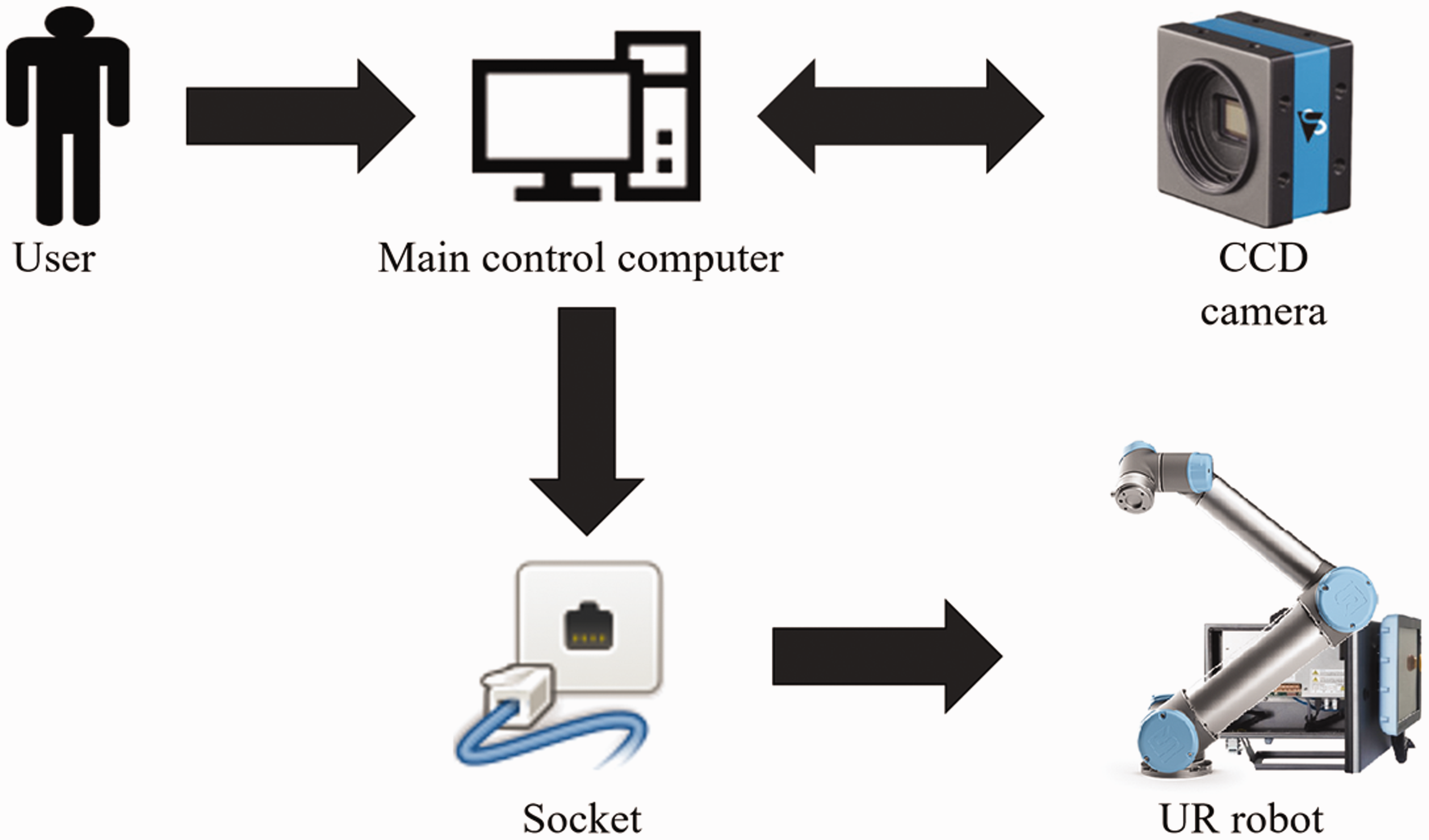
System framework of hardware commands.
Robotic arm kinematics
The first step in robotic arm operation is accurate marking of the target object position as well as the relative position of the robotic arm to the target object. In other words, the orientation relationship between them must be determined. After gaining the necessary information about the coordinates, each stage of coordinate transformation can be carried out. Kinematics is used to describe the tracking of an object in motion and involves forward and inverse kinematics. 17 Forward kinematics determines the robotic arm pose and end point via the rotational angle of each axis joint. Inverse kinematics back calculates the joint angle of each axis from the robotic arm pose and end point position. Forward kinematics is the basis of inverse kinematics and can be used for checking the correctness of inverse kinematics. In industrial applications, a series of end point positions are often given. Inverse kinematics is used to determine the corresponding joint angle of each axis to each position and to control the motors, so that each joint can reach the determined position. This allows the robotic arm to complete each given pose. The kinematic relationship is shown in Figure 2.
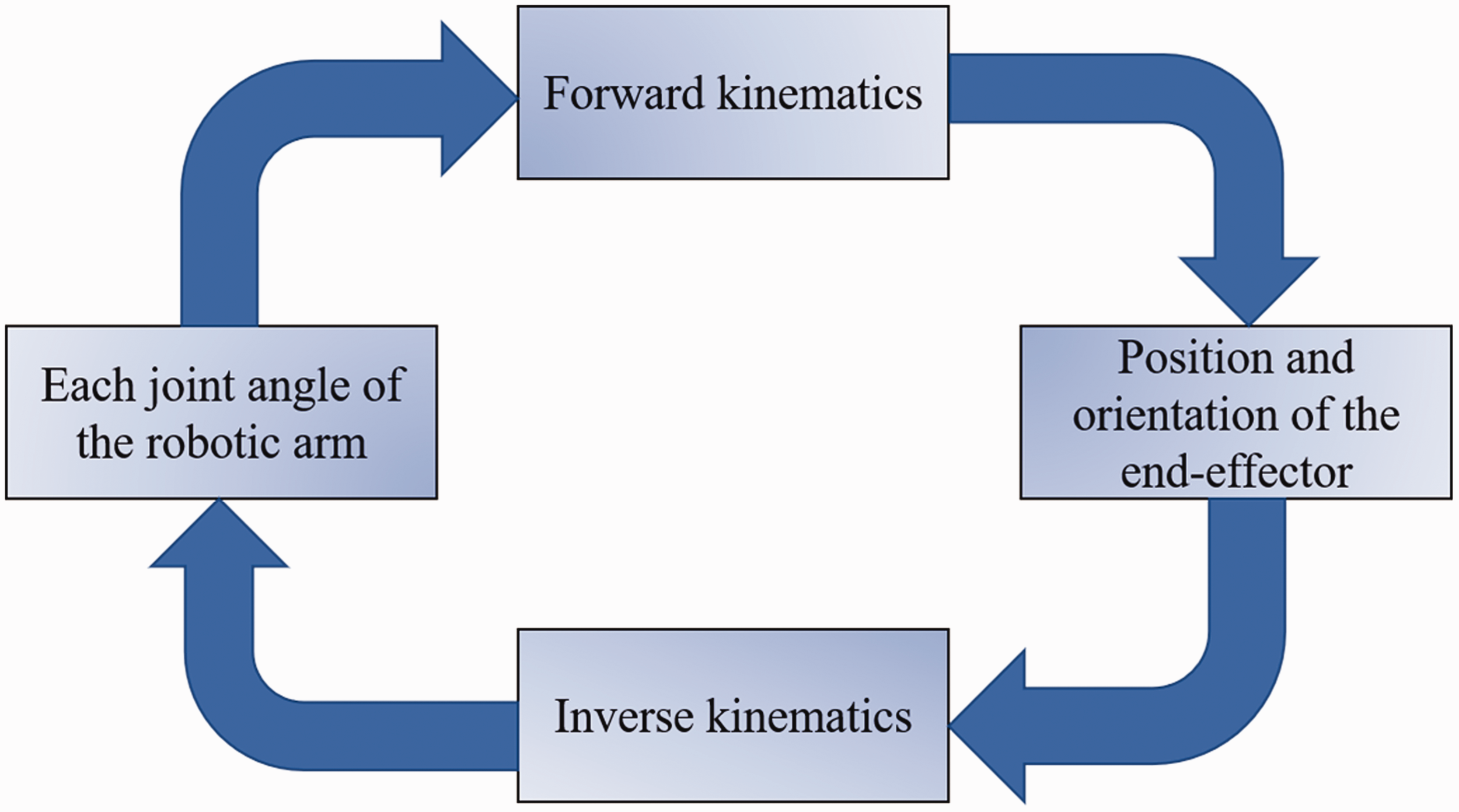
Kinematic relationship structure.
The D–H forward kinematics robotic arm coordinate system
Forward kinematics involves sending position angle information to the controller for each joint to establish a position. In the D–H coordinate method, appropriate parameters are defined which make originally complex transformation simple and clear. The UR5 robot positions and local reference coordinates of each axis joint18–21 are shown in Figure 3.
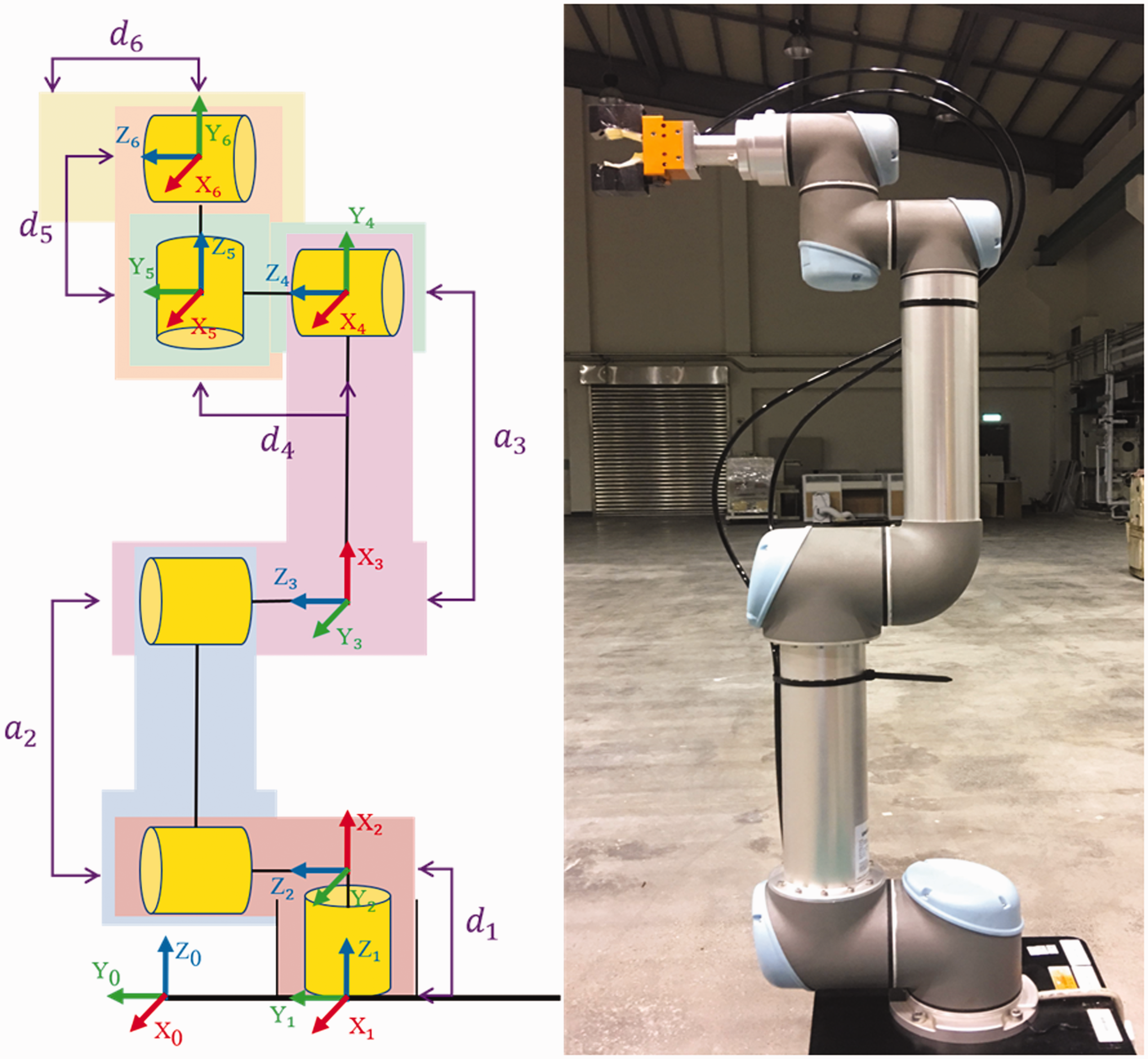
UR robot positions and local reference coordinates of each joint.
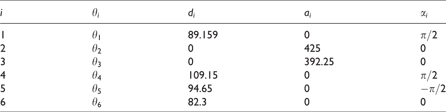
Standard D–H parameter, i-robotic arm axis joint,
UR robot D–H parameters.
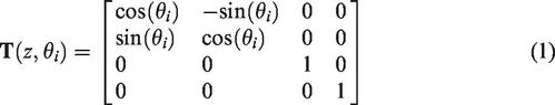
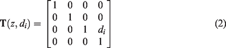
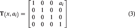
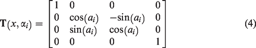
Via the D–H transformation matrix, equations shown in equations (1) to (4)
Therefore, the result of each axis via the coordinate system transformation matrix 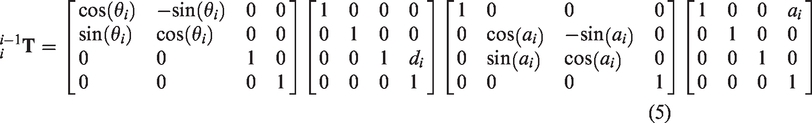
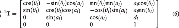
It is shown in equation (6) after rearranging equation (5)
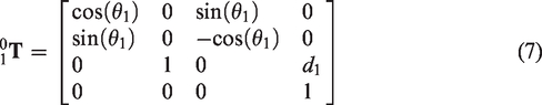
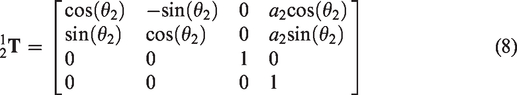
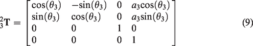
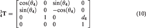
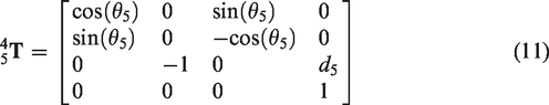
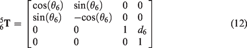
By combination with the (Table 1) UR robot D–H parameters, we can determine the transformation matrix of each axis joint as shown in equations (7) to (12)
Finally, the transformation matrix is determined as shown in equation (13)
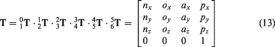
After simplification, the parameters are as in equation (14)
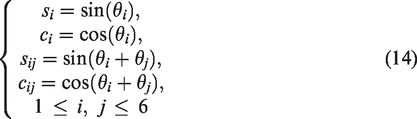
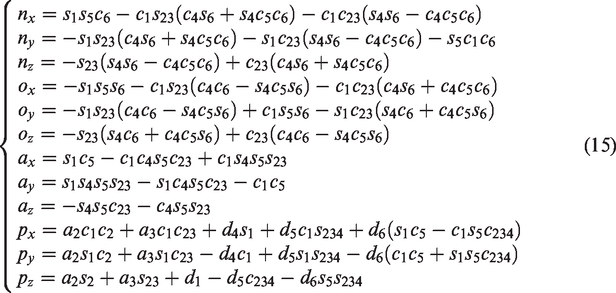
When all 
Robotic arm inverse kinematics
If the pose of the robotic arm end point relative to the machine base coordinate is known, we can back calculate the joint angle 
Since 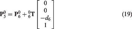
Since 
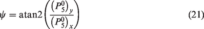

The planar projection of the fifth axis joint coordinate to the base coordinate.
Since 
From Figure 5, we can determine 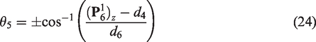
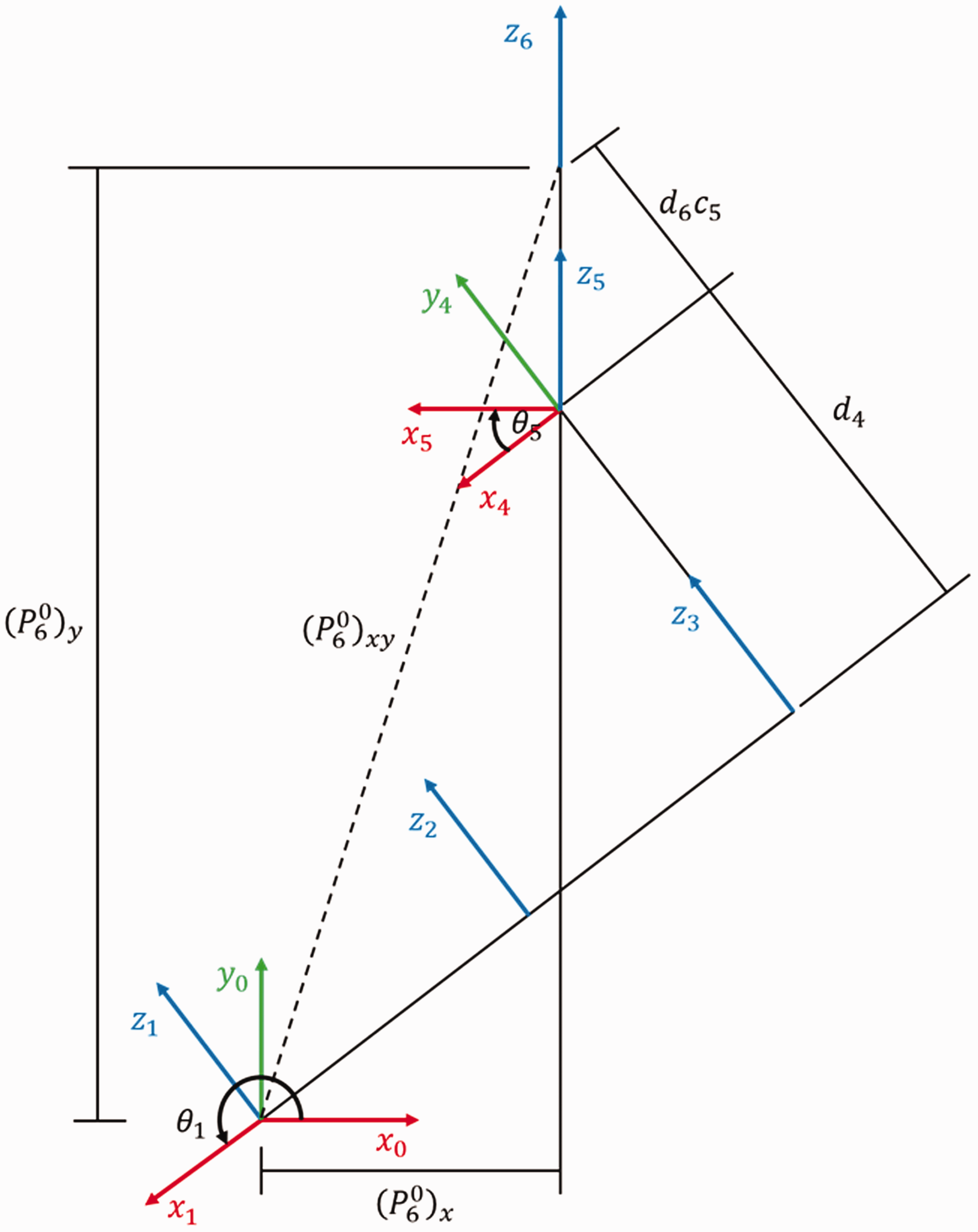
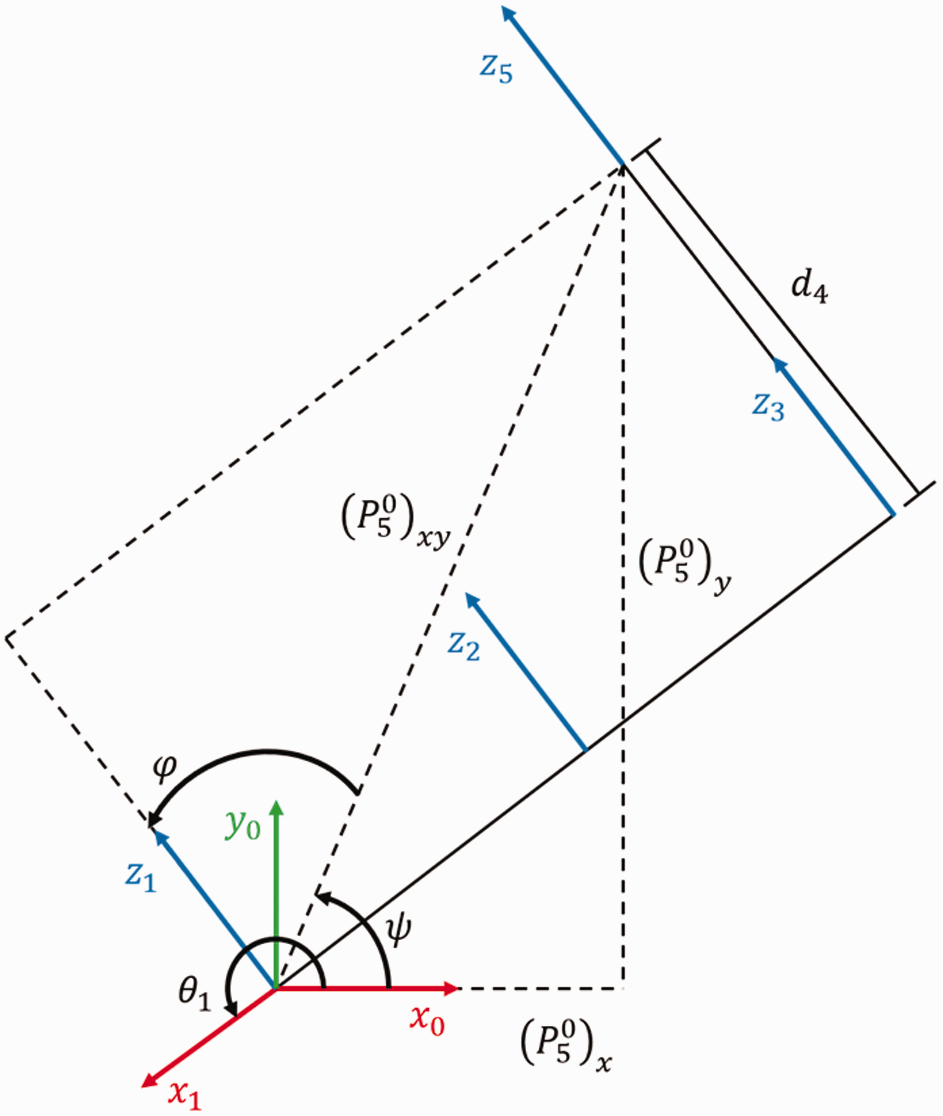
The planar projection of the sixth axis joint coordinate to the base coordinate.
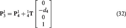
Since 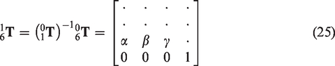


Therefore, when 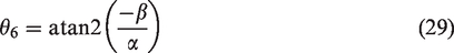
When 

Now, 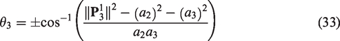
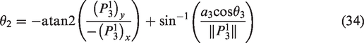
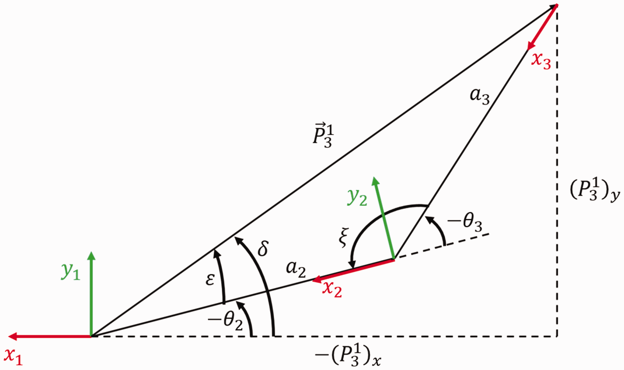
The planar projection of the fifth axis to the first axis joint coordinate.
When 
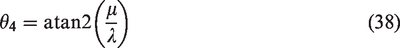
Last, using equations (36) and (37), we can determine 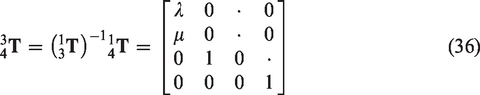
Analysis of the kinematic singularity
The six-axis robotic arm is driven by six individual motors that provide axial motion at each axis. The arm has six degrees of freedom in 3D space. Theoretically, the end point position of the six-axis robotic arm can reach any position and angle in 3D space. However, it can still get stuck in certain positions because some singularities remain. When it is located at a singularity, inverse kinematics can fluctuate. This poses a potential danger to later tracking planning. When the end point is near a singularity, a minute displacement change can cause a dramatic angle change to some axes. This can generate an approximate infinite angular velocity. If the inverse kinematics of the arm has a solution in the analytic form,
24
then it is possible to find the possible singularities by judging the abnormal condition where the denominator of the algebraic form of the solution is zero. When the value of the matrix determinant of the arm is zero, the robotic arm is located at a singularity. If the second, third, and the fourth axis are in parallel, in an arm with six degrees of freedom, the solution in analytic form that exists in inverse kinematics is given by equation (29), and when
Hough transformation and mass center calculation
In this study, the Hough transformation method was used to find the location of the image of the workpiece to be gripped and also to determine the mass center of the workpiece. After processing, this information was transferred to the robotic arm controller to complete the gripping task.
The Hough transformation, also called Hough gradient method, is a special detection method widely used in digital image processing and computer vision analysis. The Hough transformation uses binarization to identify specific lines in the image. The theory is the location of line parameters using the positions of all the points in the image. One-to-many mapping of each point in the image to the parameter space is used to get the possible parameter values. The parameter values generated by all points are accumulated to determine the line parameter that presents most obviously in the parameter space.
The thinking behind the Hough circular transformation29–32 is that each non-zero pixel point is likely to be a point on a circle, and an accumulated coordinate plane is generated by voting. The position of the circle is determined by setting up an accumulated weight. On the line coordinate, the circular equations of all points on the same circle are the same. Therefore, when mapping to the 3D space Cartesian coordinate system, also known as the abr-coordinate system, they will be the same point. Therefore, by judging the accumulated intersections of each point in the abr-coordinate system, the points greater than a certain threshold value are circles. Any straight line that passes and holds a right angle to the circumference will intersect and be perpendicular to a point. The intersection of the points is the center of the circle. The threshold value can be judged from the number of intersections on the circle center, as shown in Figure 7.
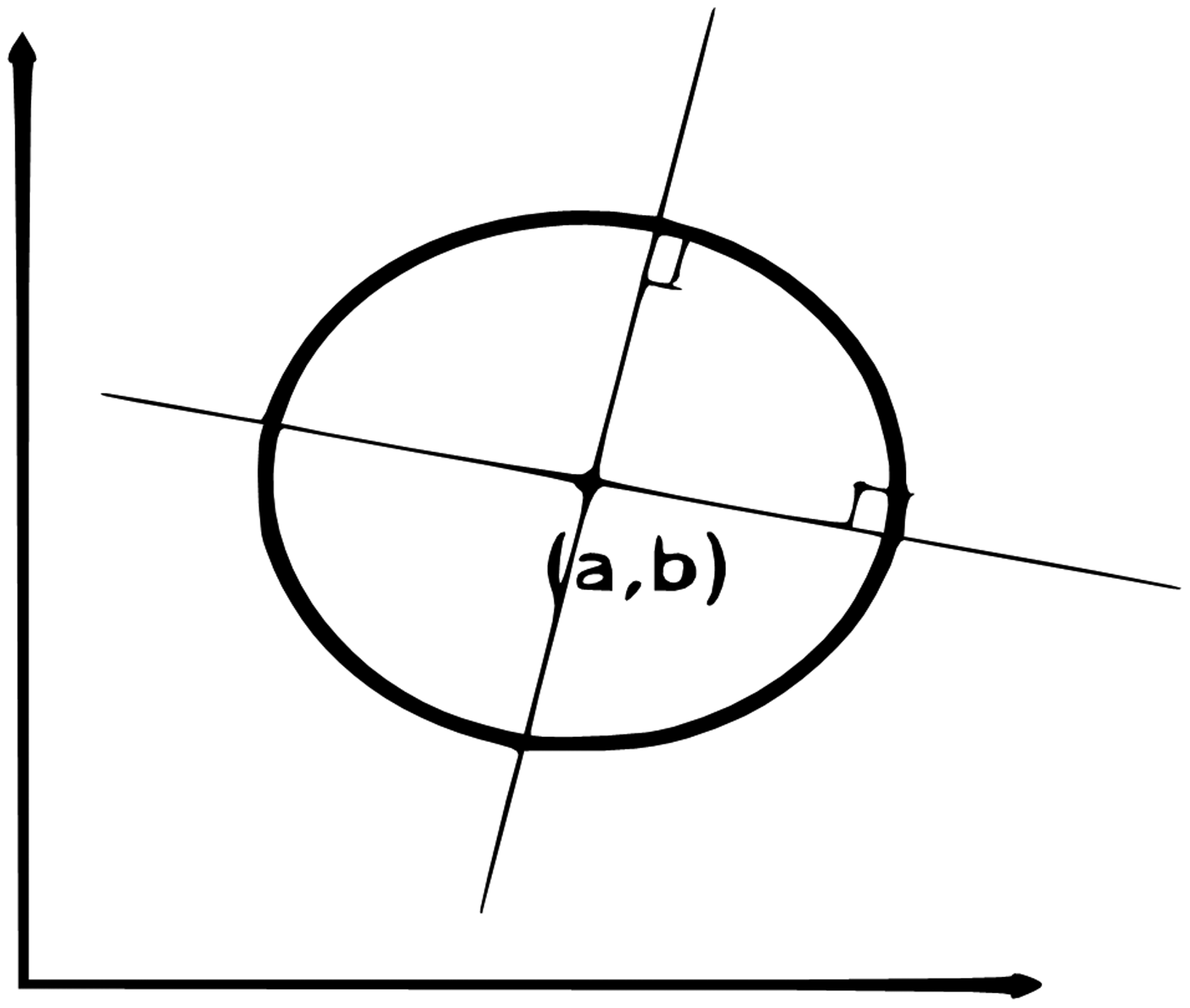
Schematics of Hough circular transformation.
For a standard Hough transformation,
33
three parameters are needed to describe a circle, the circle center, and the radius (a, b, r). Any point (x, y) in the image space can be mapped to 3 D space (a, b, r) to form a circular cone as shown in equation (39)

Look for a possible circle center for the point on each edge and build a 3D circular cone accumulator by using the edge as the circle center. These circles will overlap on the target circle center. Last, find the circle center and the radius from the point with most overlap. The circle can be expressed as in equation (40)

Analyze any pixel point in the graph corresponding to the graph in 3D space. If the radius r is certain, the pixel point corresponding to the 3D space will be a circle. If the radius r is not certain, then any shape with the radius r must be a circle. This circle will form a 3D circular cone as shown in Figure 8.
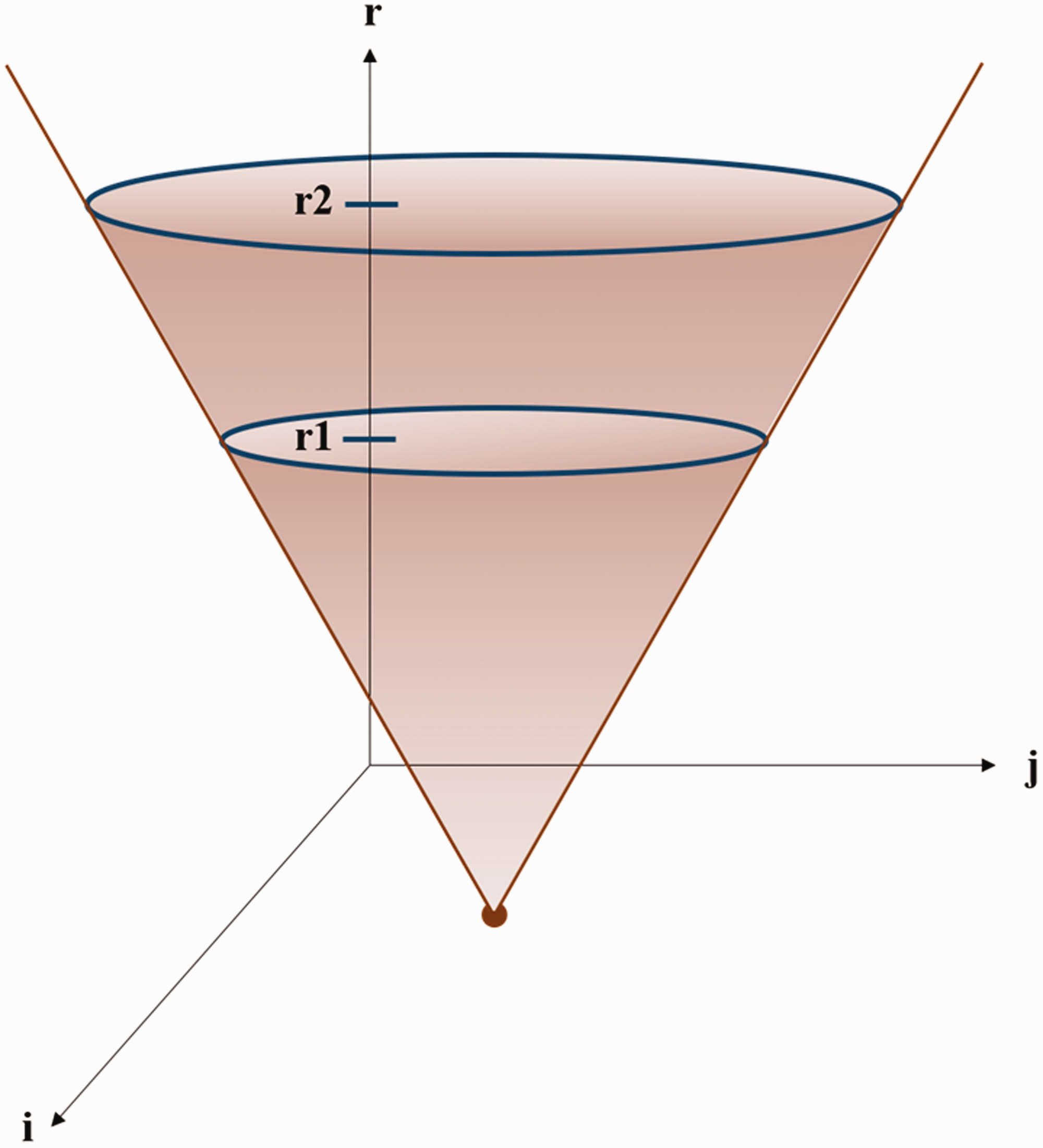
Schematics of a circular cone from the Hough transformation.
If a line is drawn along the gradient direction from any point on the circle, then the intersection of all lines may possibly be the circle center. First, calculate the possible circle center. Then, calculate the possible radius with the circle center. The circle that is checked must have a boundary. Detect the edge with the Sobel operator.34,35 Technically, the Sobel operator is a discrete difference operator used to find the approximate gradient value of the graphic brightness function. This operator includes two sets of
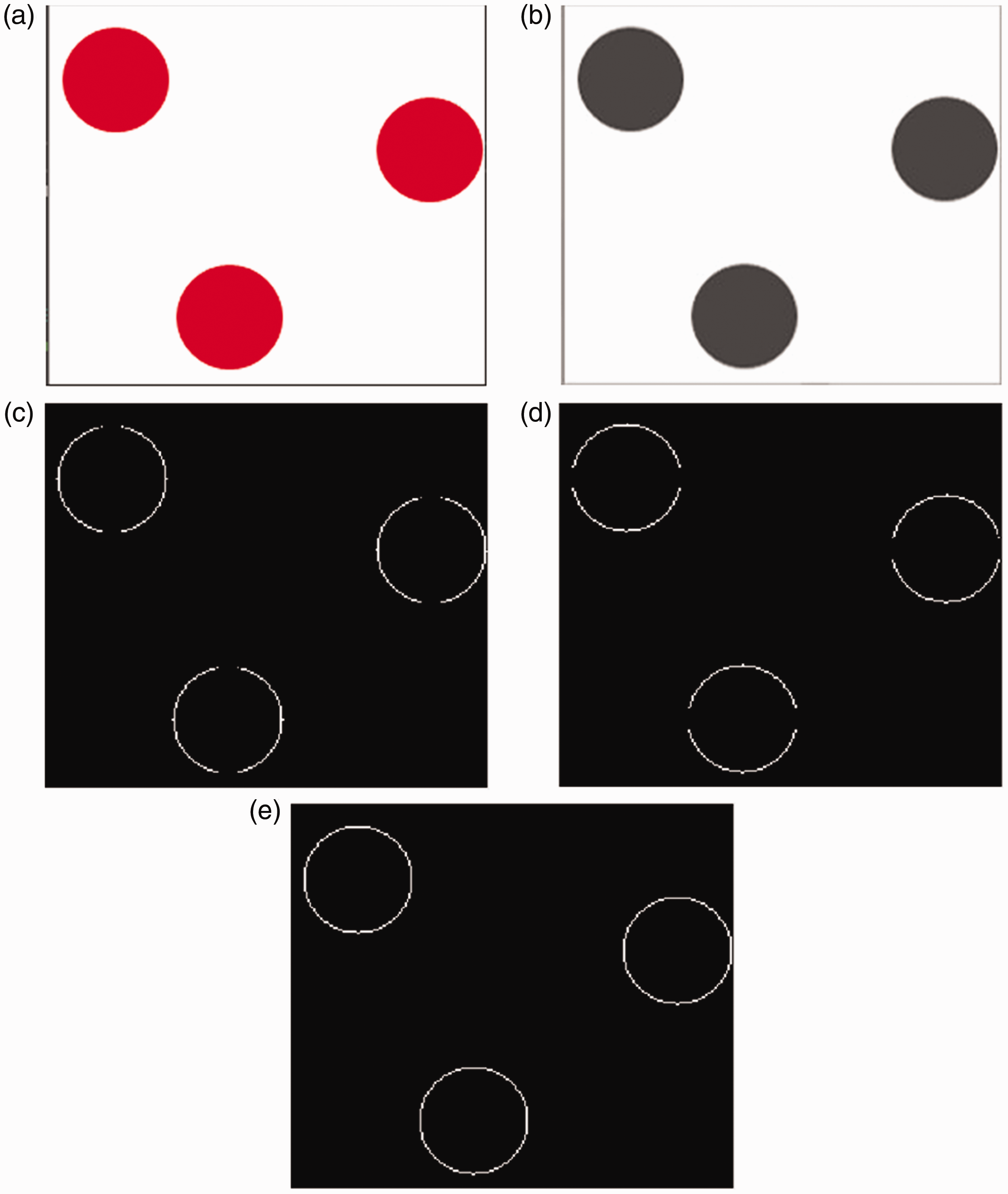
Detection of the circle: (a) original image; (b) grayscale image; (c) horizontal gradient via Sobel processing; (d) vertical gradient via Sobel processing; (e) Integration of Sobel horizontal and vertical gradients.
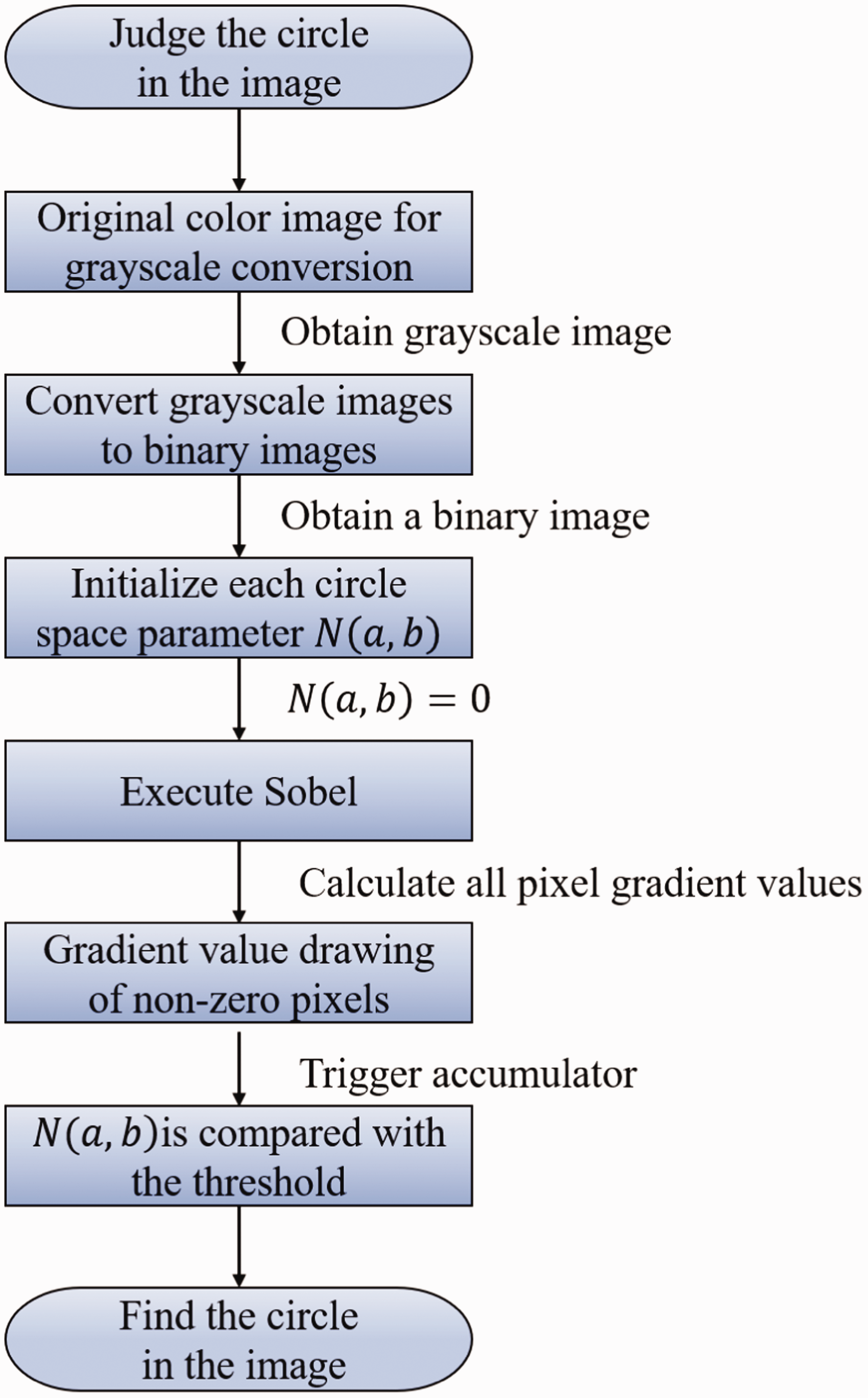
The circle detection process.
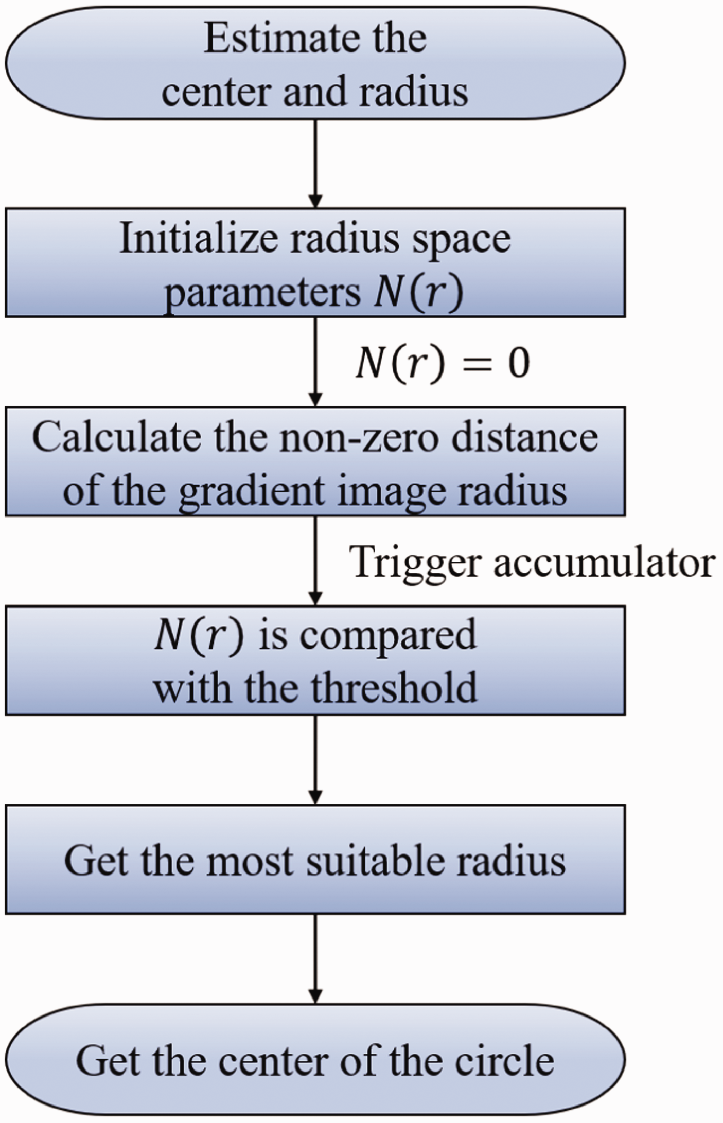
Circle radius and circle center estimation flowchart.
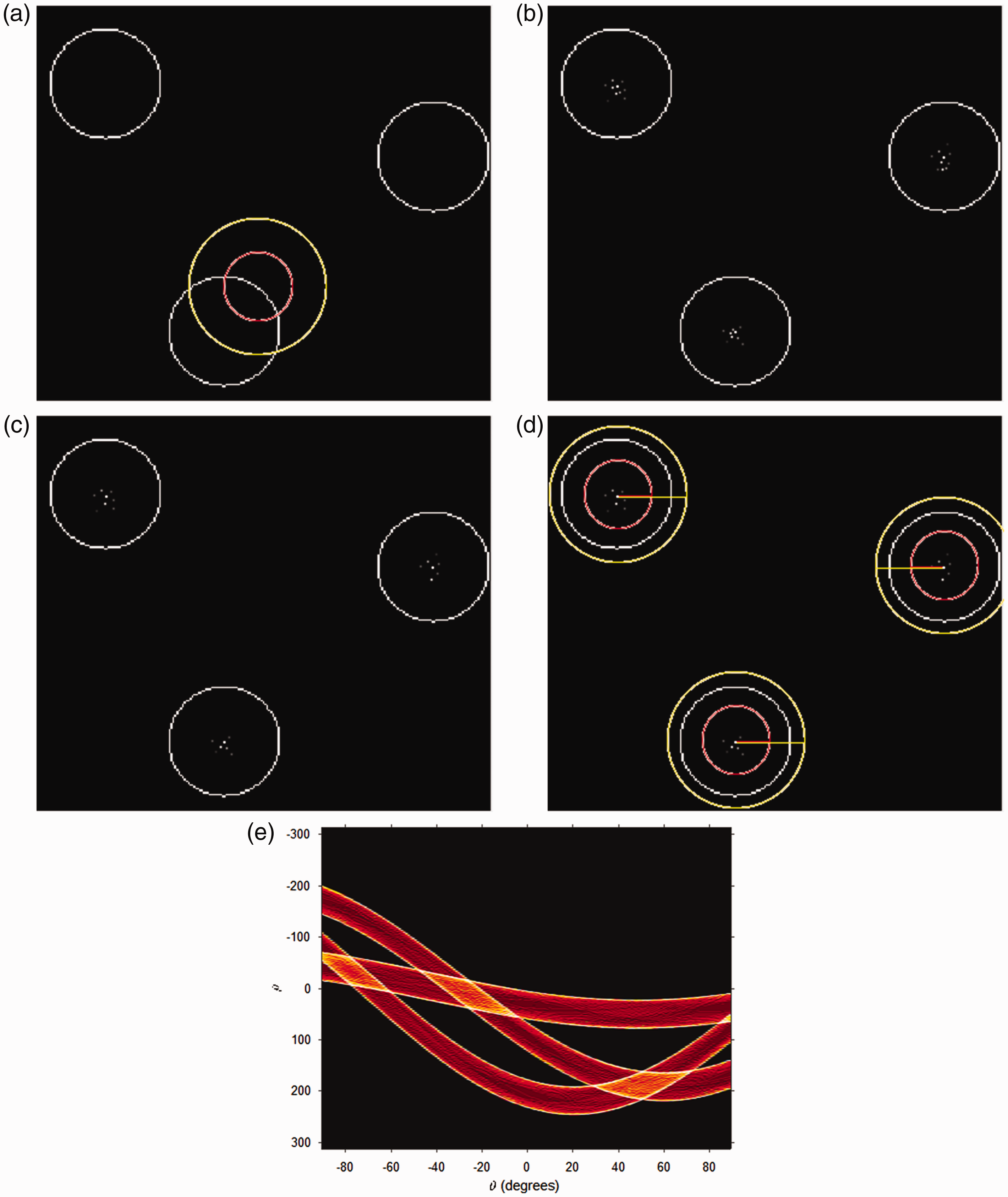
Circle radius estimation: (a) detect the radius in the positive and negative gradient directions; (b) assumed circle centers; (c) remove some circle centers; (d) seek the optimum circle center; (e) Hough space.
The original color image (Figure 9(a)) processes the original image into a grayscale image (Figure 9(b)). Then, the Sobel operator is used to get the horizontal and vertical gradients (see Figure 9(c) and vertical (Figure 9(d)). Finally, the horizontal and vertical gradient values are combined to find the center point (Figure 9(e)).
Figure 10 demonstrates the Detection Circle Process. First, the original color image is converted to grayscale and binary images are obtained from them. The Sobel operator is then used to obtain horizontal and vertical gradient values, which are then mapped to the
Figure 11 illustrates the Circle Radius and Circle center Estimation Flowchart. The radius of each gradient value obtained from the gradient image is detected, and the value obtained from detection is saved in the
Movement in the positive or negative directions of the gradient is made to carry out detection within the range of the radius, see Figure 12(a). The points recorded after detection are assumed to be the center of circles, see Figure 12(b), and comparisons will result in the strongest being left, see Figure 12(c). Last, the radius using some of the assumed circle centers is calculated to find the optimum circle (Figure 12(d)). Last, Hough transformation is used to obtain the space graph, see Figure 12(e).
After obtaining the optimum circle, we can get the planar transform relationship between the workpiece to be gripped and the current image. The center of this circle can also be defined as the mass center. The mass center is the reference point for control, and its 2D planar coordinates represent the position of the workpiece to be gripped. The robot arm can now be directed to complete the gripping task.
Communication method-socket
To satisfy the communication requirements36,37 for the robotic arm system, and to achieve support for some TCP/IP functions that are not easy to integrate into the prevailing function library (TCP/IP Protocol Suite), we define some system call functions—Socket Interface. The Socket web framework is shown in Figure 13. The TCP/IP Socket protocol used in this study forms a satisfactory link between the PC end and the controlled end of the robotic arm.
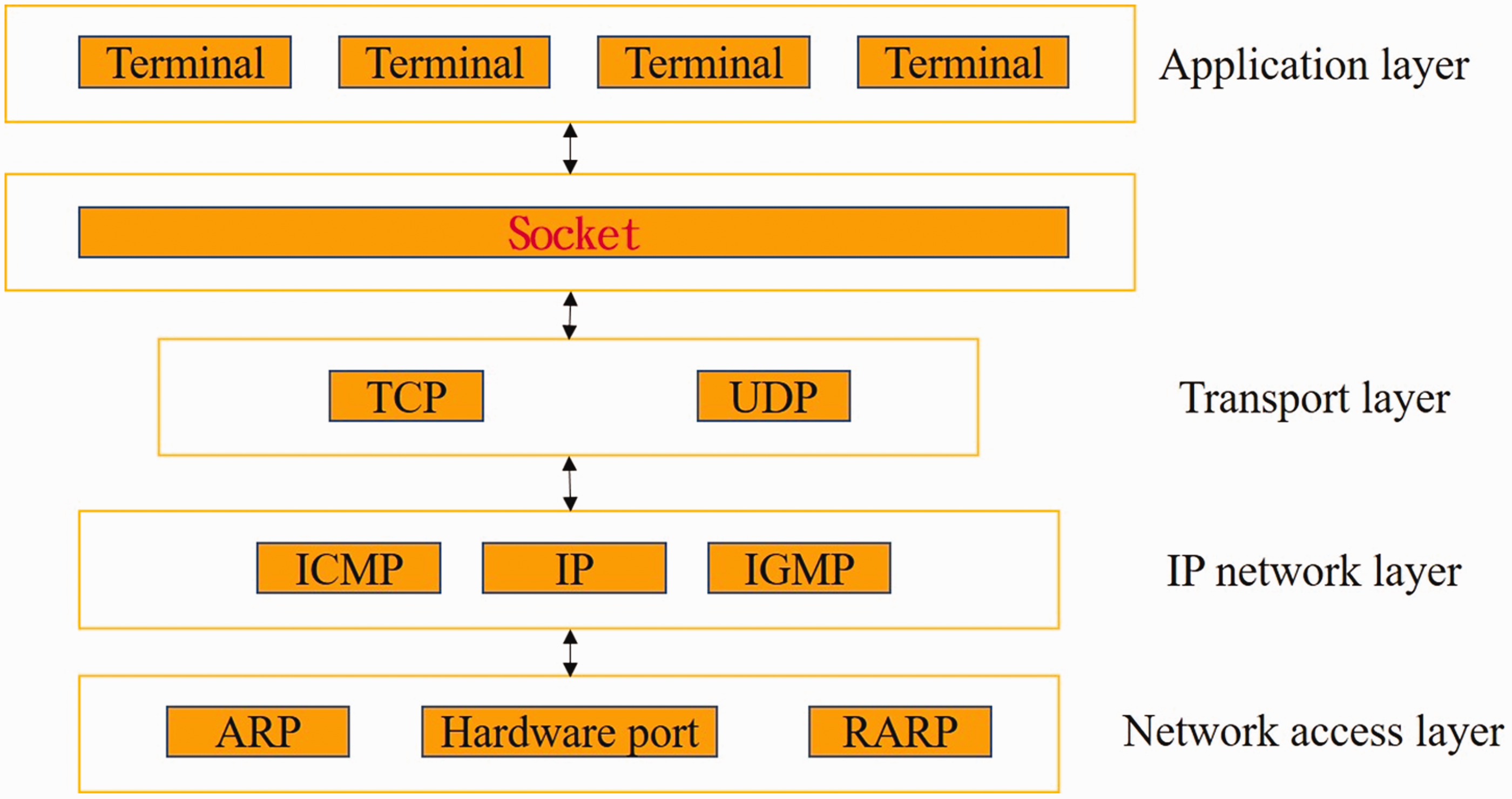
Socket web framework.
The application layer is similar to that used by other network applications such as Telnet, FTP, WWW, POP Email, News, and BBS. The transport layer is responsible for network connection, division, and combination for transmitting messages and for providing control for data traffic between usage nodes. It also decides the service quality and provides reliable and efficient connection for network application nodes. The IP network layer receives the packets sent from the transport layer. Transmission is automatically routed to the address, and packet format can be changed to that of a different protocol, the network traffic condition is monitored, and an overall network topology framework is dynamically built to provide the best route for data transmission. The network access layer receives the packets sent from the IP network layer to divide, combine, and detect the data frame in more detail and correct errors, and ACK is used to determine whether the data is transmitted normally and controls the transfer rate. It is responsible for transmitting the original network data formed between 0 and 1. The method used in this study was TCP/IP. Socket is a port used for network communication in the UNIX system. In general program operation, it can be regarded as an operation for File I/O. Basically, this relies on two key points: read and write. How to read the incoming data and how to write the output. The basic steps before performing these operations are shown in Figure 14.
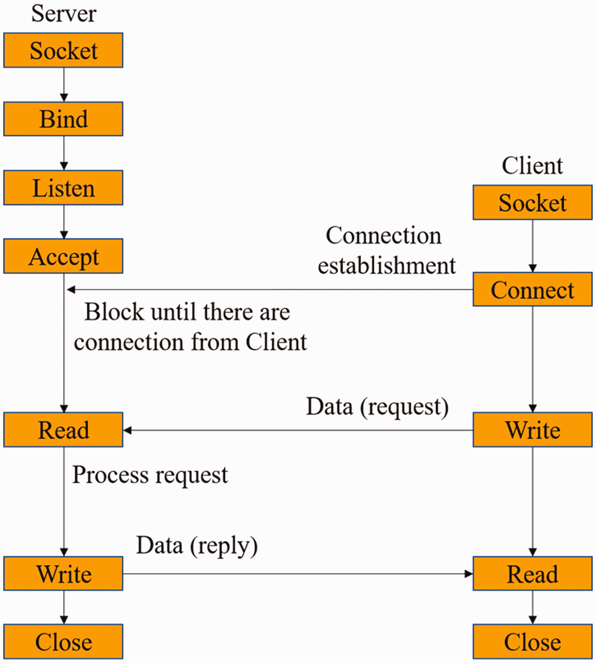
Socket flowchart.
Experimental results and discussion
Details of the experimental flowchart are shown in Figure 15. An image of the object is acquired by the CCD camera and transferred to the PC via the USB connection. The Hough transformation method is used to analyze and compute the information until the workpiece to be gripped is found as shown in Figure 16. The actual flow is from the original RGB image input (Figure 16(a)) which has been reduced to grayscale (Figure 16(b)) to reduce its computational complexity and the SOBEL level (Figure 16(c)), vertical detection of the image (Figure 16(d)) has been started and integrated (Figure 16(e)), the gradient values have been converted into the Hough space (Figure 16(f)) to determine if it is a circle, and finally, the circle identification (Figure 16(g)) has been completed. The mass point of the object is then found by calculation and the D–H coordinate system transfers this information (by the socket method) to the UR5 robot controller. The robotic arm carries out the necessary movement to grip the workpiece. It automatically moves to the correct position and completes the movement as shown in Figures 17 and 18.
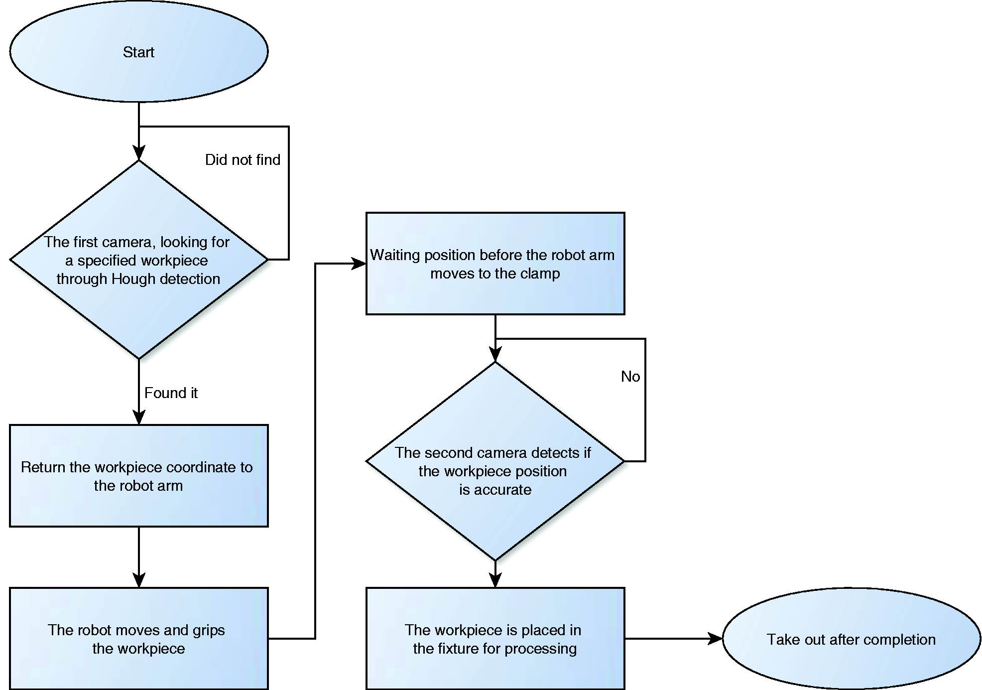
Experiment flowchart.
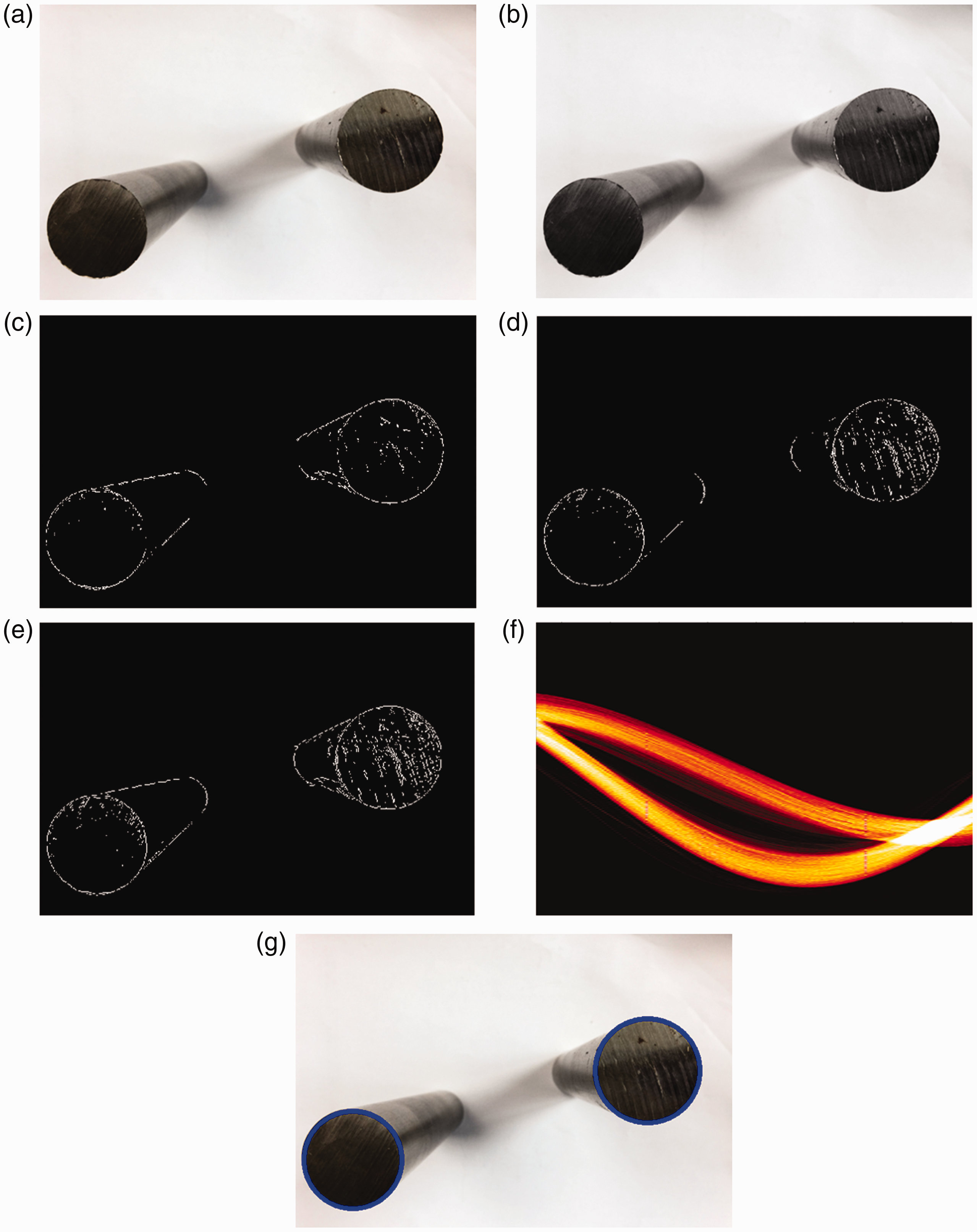
Finding the workpiece using the Hough transformation: (a) original image; (b) binary image from grayscale; (c) horizontal gradient from Sobel; (d) vertical gradient from Sobel; (e) integration of horizontal and vertical Sobel gradients; (f) Hough space; (g) finding the workpiece.
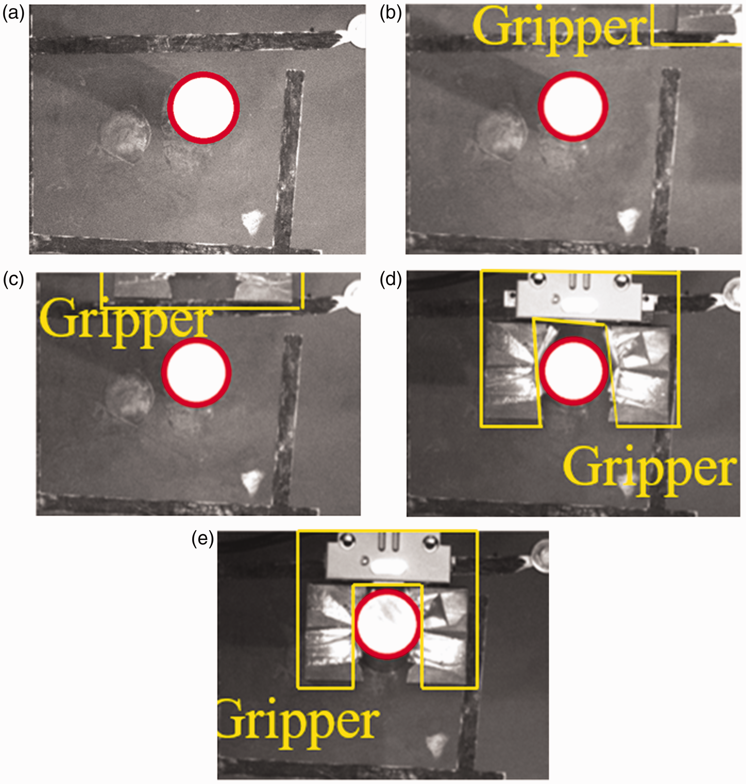
Separate images for gripping: (a) find the workpiece to be gripped; (b) move arm to waiting point 1; (c) move arm to waiting point 2; (d) move arm to workpiece position; (e) grip the workpiece.
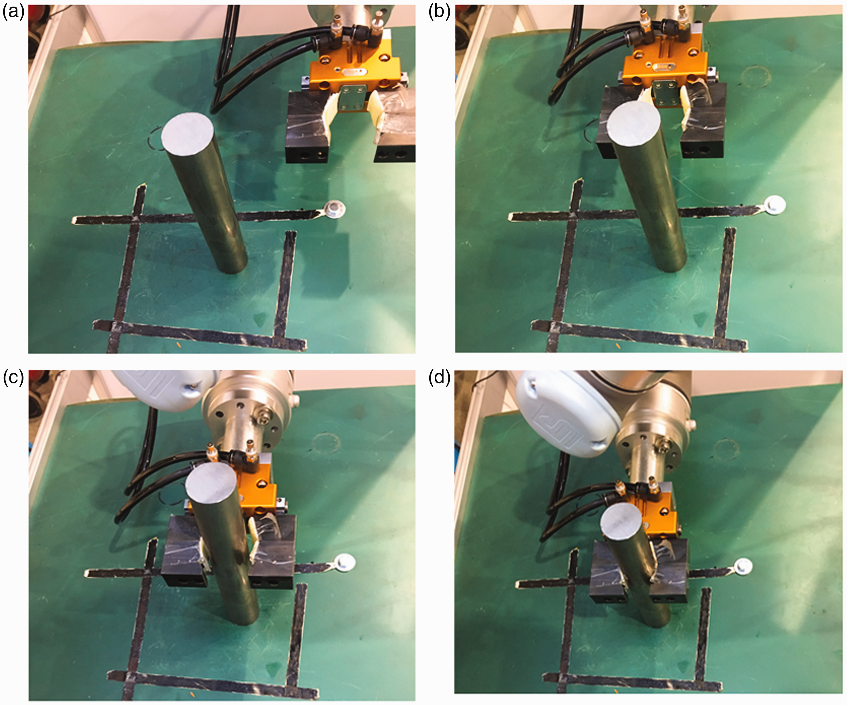
Gripping by the robotic arm: (a) move arm to waiting point 1; (b) move arm to waiting point 2; (c) move arm to the workpiece position; (d) grip the workpiece.
After the workpiece has been gripped, the robot arm receives commands (via Socket) to move to the fixture position where the workpiece is to be placed as shown in Figure 19. The second CCD camera provides information for visual identification, and any deviation between the workpiece being held by the arm and the fixture will automatically be corrected. After this, the work continues, and the workpiece is placed smoothly into the fixture. The workpiece is finally picked out of the fixture after machining has been done. The system described here also has a user-friendly man-machine interface for monitoring the operations.
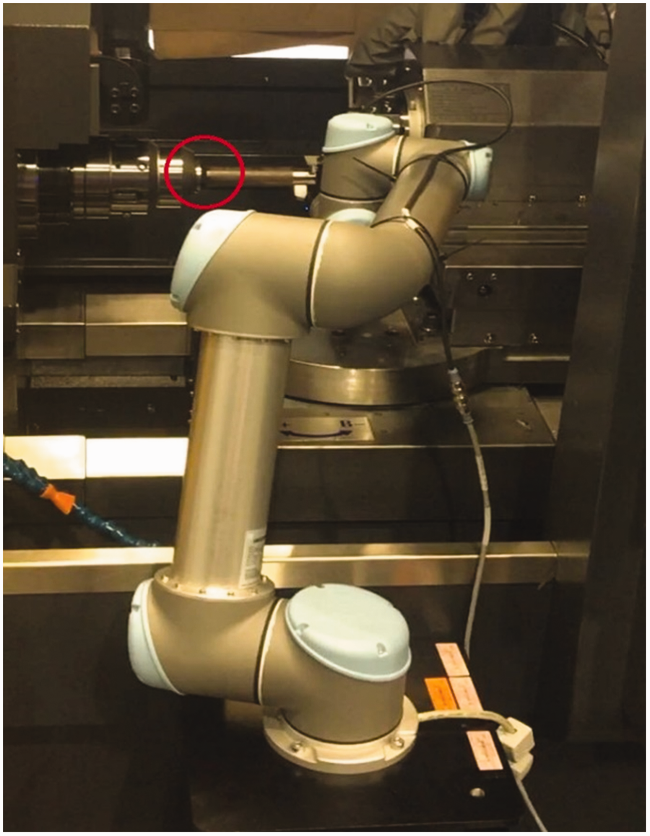
Automatic error calibration using Hough transformation.
The Hough transformation is used to identify the workpiece to be clamped on the captured image (Figure 17(a)). The robot arm moves to waiting point 1 (Figures 17(b) and 18(a)). After the centroid of the workpiece is found, the coordinate of the workpiece to be selected is sent to the UR5 robot arm using the Socket method, and UR5 robot arm is moved to the first position, point 1. After a wait at point 2 (Figures 17(c) and 18(b)), it finally moves to the workpiece position (Figures 17(d) and 18(c)) to capture the workpiece (Figures 17(e) and 18(d)).
The Hough transformation is useful for recognizing the specific lines of an image by binarization and uses all the pixel points in an image to find the parameters of a straight line. Each point obtains its parameter value by one-to-many projection to the parameter space, and parameter values are generated by all the points to find the most obvious line parameter in the space. The Generalized Hough Transformation does not have much influence on image distortion or pixel loss and is not limited to the recognition of straight lines. In fact, it can be used to recognize any shape. However, it cannot make an efficient classification, and the outcome is not stable enough for computer vision. The parameter space used to search for the target can become very large in a short time, and a lot of storage space is needed. However, the Hough transformation can solve the above-mentioned problems, and it was chosen for this study.
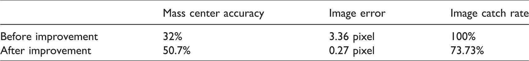
It can be seen in Table 2 that after improvement, the Hough transformation method can quite accurately locate the mass point of the workpiece to be gripped. The pixel error for the mass center was also reduced by 3.09 pixels. However, the catch rate, when compared to the method before improvement, was reduced by 26.27%. However, the time for image acquisition (before the robotic arm grips the workpiece) is more than adequate for the Hough transformation to determine the mass center of the workpiece to be gripped. Therefore, image recognition, as performed by our improved Hough transformation method, was used in this study.
Hough transformatin method comparison.
Conclusion
In this study, communication between the “image” and the robotic arm was proposed to reduce preexisting errors in location. Integration of the robotic arm and image identification allowed automatic judgment to be made without the need for an extra manipulator. Correction of the inherent errors and accurate calibration was achieved via feedback vision. This allowed the endpoint pose position of the arm to be fine-tuned, and this significantly improved its accuracy. Measurements were made with the highly stable Hough transformation method rather than by the in-depth mechanical learning methods used before. Hough transformation works without the need to build a huge database of training data and saves a lot of time. Results showed that changing the parameters to increase the Hough transformation accuracy not only reduced image pixel error but also increased the precision with which the mass point position could be determined and gave better gripping performance.
Footnotes
Declaration of conflicting interests
The author(s) declared no potential conflicts of interest with respect to the research, authorship, and/or publication of this article.
Funding
The author(s) disclosed receipt of the following financial support for the research, authorship, and/or publication of this article: This study was supported by the Ministry of Science and Technology under Project number: MOST 107–2218-E-167–001.