Dynamic response of a piecewise linear single-degree-of-freedom oscillator with fractional-order derivative

Abstract

In this paper, the dynamic response of a piecewise linear single-degree-of-freedom oscillator with fractional-order derivative is studied. First, a mathematical model of the single-degree-of-freedom system is established, and the approximate steady-state solution associated with the amplitude–frequency equation is obtained based on the averaging method. Then, the amplitude–frequency response equations are used for stability analysis, and the stability condition is founded. To validate the correctness and precision, the approximate solutions determined by the analytical method are compared with the solutions based on the numerical integration method. It is found that the approximate solutions and the numerical solutions are in excellent agreement. Finally, the effects of system parameters, such as fractional-order coefficient, order, clearance, and piecewise stiffness, on the complex dynamical behaviors of the piecewise linear single-degree-of-freedom oscillator are studied. The results show that the system parameters not only influence resonance amplitude and resonance frequency but also affect the size of the unstable region.

Introduction

Piecewise linear elastic systems are common in engineering practice due to the clearance and backlash existing in such systems. Piecewise linearity produces strong nonlinearity and discontinuity, which may affect the performance and reliability of actual systems. Many scholars have extensively studied this issue. Xu ¹ investigated the general form of periodic solutions in a system with piecewise linear viscous damping by the incremental harmonic balance method. Wang ² studied the dynamic response and stability of a single-degree-of-freedom (SDOF) system with asymmetrical piecewise linear/nonlinear stiffness using the finite element method in the time domain. Natsiavas ³ analyzed the dynamics of piecewise linear oscillators with van der Pol-type damping. Shaw and Holmes ⁴ analyzed the harmonic, subharmonic, and chaotic motions existing in a piecewise linear oscillator. Li et al. ⁵ investigated the homoclinic bifurcations and chaotic dynamics of a piecewise linear system with periodic excitation and viscous damping. Gao and Chen ⁶ studied the resonance and stability for a SDOF system with a piecewise linear/nonlinear stiffness term. Narimani et al. ⁷ analyzed a piecewise linear system and provided a complete analytical solution that agreed with numerical simulation and experimental measurements. Jiang and Wiercigroch ⁸ investigated a soft impact oscillator, and several bifurcation scenarios near grazing bifurcation have been studied. Li and Ding ⁹ considered a vibro-impact system subjected to harmonic excitation with two asymmetric clearances with semi-analytical method. Many authors have^10,11 analyzed the isolation effect of nonlinear isolator with linear elastic support boundary condition.

In such non-smooth dynamical systems, the systems themselves have various nonlinearities that affect the dynamic behavior. Fractional derivatives can accurately describe the essential properties of viscoelastic materials. Shen et al.^12–15 studied the vibration of several oscillators with fractional-order derivative, and found that the fractional-order derivatives had equivalent damping and equivalent stiffness effects on the system response. Wen et al.^16,17 investigated the dynamical analysis of different Mathieu equation with a fractional-order derivative. The research on piecewise linear oscillators with fractional derivatives is little. Due to the complexity of fractional-order calculus, most authors adopted numerical methods in this field. Yang et al. ¹⁸ explored stochastic bifurcations of a vibro-impact oscillator with fractional derivative elements driven by Gaussian white noise excitation. Danca ¹⁹ simulated and analyzed three piecewise continuous chaotic systems of fractional order. Marius et al. ²⁰ investigated a new piecewise linear fractional-order Chen system by a numerical method. Lu ²¹ numerically investigated the chaotic behaviors of the fractional-order Chua’s circuit with piecewise linear/nonlinearity. Wu et al. ²² investigated the chaotic structure of a new fractional piecewise linear system by numerical method. Such techniques can provide solutions only for specific parameters. When the range of the parameters is large, the workload is especially large.

In this work, an elastic impacting problem of viscoelastic materials with clearance is studied by means of an analytical method. The elastic impacting vibration system of this viscoelastic material is simplified as a symmetric piecewise linear system. The effects of the clearance, piecewise linear parameters, and fractional-order parameters on the vibration performance of the system are discussed. Moreover, the correctness of the research method is verified by a comparison of the analysis and numerical results.

Equation of motion

A piecewise linear SDOF oscillator with fractional-order derivative shown in Figure 1 is considered.

Figure 1.

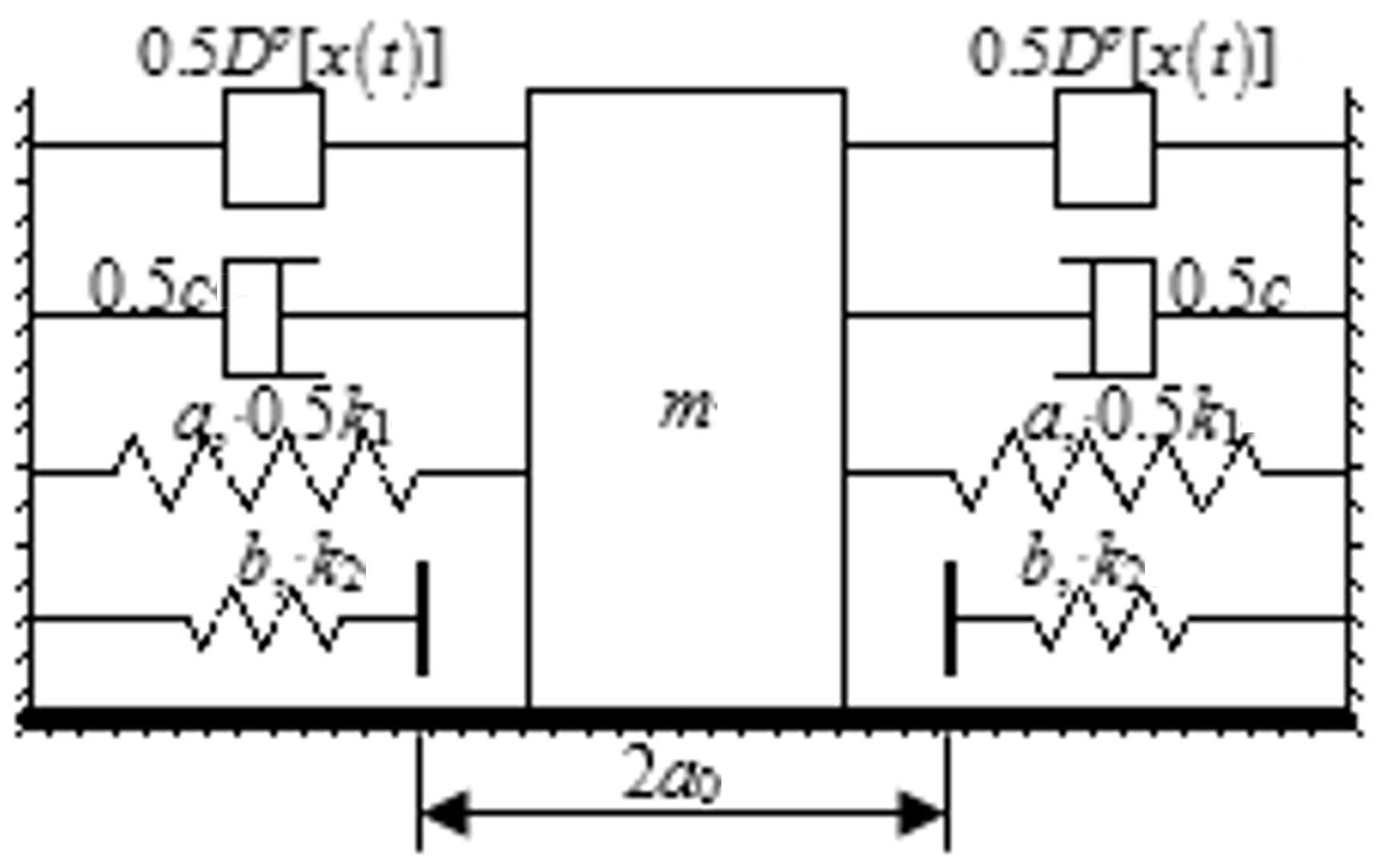
Piecewise linear SDOF oscillator with fractional-order derivative.

In this model, m, $k_1$ , and $k_2$ are the mass and stiffness coefficients for springs a and b. Mass m and spring a are linked together, but a₀ is the clearance between spring b and mass m at the equilibrium position. When the response amplitude is less than clearance a₀, only spring a is involved. When the amplitude is greater than a₀, mass m will be in repeated contact with spring b. Fractional-order derivative comes from the materials which have memory property, ¹⁸ such as metal springs, air springs, or MR dampers. The force–deformation relationship of viscoelastic materials can be expressed as $F=K_1{D}^p\left[x\left(t\right)\right]$ . F is the force, $x\left(t\right)$ is the deformation of the oscillator m, $D^p\left[x\left(t\right)\right]$ is the p-order derivative of x(t) about t, where the fractional orders are restricted as 0<p < 1, and K₁ is the fractional coefficient (K₁>0). The differential motion equation could be established as

$$m\ddot{x}\left(t\right)+k\left(x\right)+c\dot{x}\left(t\right)+K_1{D}^p\left[x\left(t\right)\right]=F\cos \left(\omega t\right)$$

(1)

where x designates the displacement of m, and k(x)is the piecewise linear stiffness

$$k\left(x\right)=\{\begin{array}{cc}{k}_{1}x+k_2\left(x+a_0\right)& \left(x<-a_0\right)\\ k_{1}x& \left(-a_0\le x\le a_0\right)\\ k_{1}x+k_2\left(x-a_0\right)& \left(x>a_0\right)\end{array}$$

Using the following transformation of formula

$${\omega }_0^2=\frac{k_1}{m},\epsilon \zeta =\frac{c}{m},\epsilon f=\frac{F}{m}\mathrm{，}\epsilon k_3=\frac{k_2}{m},\epsilon k_4=\frac{K_1}{m}$$

Equation (1) can be rewritten as

$$\ddot{x}\left(t\right)+{\omega }_0^{2}x\left(t\right)+\epsilon \zeta \dot{x}+\epsilon g_1\left(x\right)+\epsilon k_4{D}^p\left[x\left(t\right)\right]=\epsilon f\cos \omega t$$

(2)

$$g_1\left(x\right)=\{\begin{array}{cc}{k}_3\left(x+a_0\right)& \left(x<-a_0\right)\\ 0& \left(-a_0\le x\le a_0\right)\\ k_3\left(x-a_0\right)& \left(x>a_0\right)\end{array}$$

(3)

Approximate analytical solution

This section presents a detailed analytical procedure to find the approximate solution of the system. Different approaches had been used to find the steady-state responses of non-smooth systems with piecewise stiffness. Gao and Chen ⁶ applied a modified perturbation method to find the approximate solution of an SDOF system with a piecewise stiffness term. The averaging method, which is also commonly used in this kind of system,^23--25 is utilized to obtain the approximate solutions in the current work.

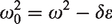
Based on the averaging method, one could obtain the standard equations. To study the primary resonance, that is, ω₀ = ω, a detuning parameter is introduced to illustrate the approximate degree between ω₀ and ω

$${\omega }_0^2={\omega }^2-\delta \epsilon$$

Equation (2) becomes

$$\ddot{x}\left(t\right)+{\omega }^{2}x\left(t\right)=\epsilon \left\{f\cos \omega t+\delta x-\zeta \dot{x}-g_1\left(x\right)-k_4{D}^p\left[x\left(t\right)\right]\right\}$$

(4)

The solution to equation (4) is considered as

$$\begin{array}{l}x=a\cos \varphi \\ \dot{x}=-a\omega \sin \varphi \end{array}$$

(5)

where $\varphi =\omega t$

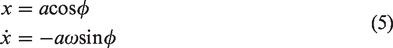
Substituting equation (5) into equation (3), one could obtain

$$g\left(a\cos \varphi \right)=\{\begin{array}{ll}{k}_{3}a\left(\cos \varphi +\cos {\varphi }_0\right)& \left(\pi -{\varphi }_0<\varphi <\pi +{\varphi }_0\right)\\ 0& \left({\varphi }_0<\varphi <\pi -{\varphi }_0,\pi +{\varphi }_0<\varphi <2\pi -{\varphi }_0\right)\\ k_{3}a\left(\cos \varphi -\cos {\varphi }_0\right)& \left(0<\varphi <{\varphi }_0\mathrm{，}2\pi -{\varphi }_0<\varphi <2\pi \right)\end{array}$$

(6)

To study the approximate analytical solution, equation (4) can be transformed into

$$\ddot{x}\left(t\right)+{\omega }_0^{2}x\left(t\right)=\epsilon f\left(a,\omega \right)$$

(7a)

$$f\left(a,\omega \right)==f_1\left(a,\omega \right)+f_2\left(a,\omega \right)+f_3\left(a,\omega \right)$$

(7b)

$$f_1\left(a,\omega \right)=\epsilon \left[f\cos \left(\varphi -\theta \right)+\delta a\cos \varphi +\zeta a\omega \sin \varphi \right]$$

(7c)

$$f_2\left(a,\omega \right)=-\epsilon {\omega }_0^{2}g\left(a\cos \varphi \right)$$

(7d)

$$f_3\left(a,\omega \right)=-\epsilon k_4{D}^p\left[a\cos \varphi \right]$$

(7e)

The averaged equation for the amplitude and phase of the approximate solutions can be obtained as

$$\dot{a}=-\frac{1}{\omega }\left[f_1\left(a,\theta \right)+f_2\left(a,\theta \right)+f_3\left(a,\theta \right)\right]\sin \varphi$$

(8a)

$$a\dot{\theta }=-\frac{1}{\omega }\left[f_1\left(a,\theta \right)+f_2\left(a,\theta \right)+f_3\left(a,\theta \right)\right]\cos \varphi$$

(8b)

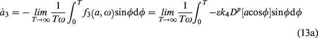
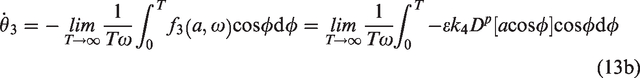
The amplitude a and generalized phase θ are slow-varying functions. One can integrate them in the interval [0 T] according to the averaging method

$$\dot{a}=-\frac{1}{T\omega }{\displaystyle {\int }_0^T\left[f_1\left(a,\theta \right)+f_2\left(a,\theta \right)+f_3\left(a,\theta \right)\right]\sin \varphi \mathrm{d}\varphi }$$

(9a)

$$a\dot{\theta }=-\frac{1}{T\omega }{\displaystyle {\int }_0^T\left[f_1\left(a,\theta \right)+f_2\left(a,\theta \right)+f_3\left(a,\theta \right)\right]\cos \varphi \mathrm{d}\varphi }$$

(9b)

The time terminal T is selected as T = 2π when f_i (a, θ) (i = 1,2) is periodic function, and T = ∞ if f₃ (a, θ) is aperiodic.

One could get the simplified forms of the first part of equation (9)

$${\dot{a}}_1=-\frac{1}{2\pi \omega }{\displaystyle {\int }_0^{2\pi }{f}_1\left(a,\theta \right)\sin \varphi \mathrm{d}\varphi =-\frac{1}{2\omega }\epsilon f\sin \theta -\frac{1}{2}a\epsilon \zeta }$$

(10a)

$$a{\dot{\theta }}_1=\frac{1}{2\pi \omega }{\displaystyle {\int }_0^{2\pi }{f}_1\left(a,\theta \right)\cos \varphi \mathrm{d}\varphi =-\frac{1}{2\omega }\epsilon f\cos \theta -\frac{1}{2\omega }a\epsilon \delta }$$

(10b)

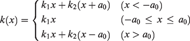
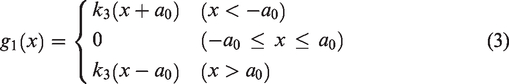
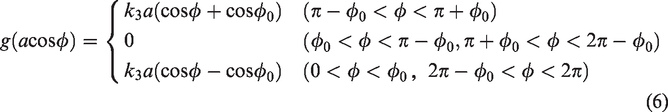
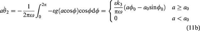
The second part of equation (9) is the piecewise linear integral. Obviously, there exist two kinds of solutions for the piecewise linear system, that is to say, a small-amplitude linear vibration (which means that the displacement does not exceed the critical displacement point a₀) and a large-amplitude nonlinear vibration which can be beyond the critical point a₀. Accordingly one can get

$${\dot{a}}_2=-\frac{1}{2\pi \omega }{\displaystyle {\int }_0^{2\pi }-\epsilon g\left(a\cos \varphi \right)\sin \varphi \mathrm{d}\varphi =0}$$

(11a)

$$a{\dot{\theta }}_2=-\frac{1}{2\pi \omega }{\displaystyle {\int }_0^{2\pi }-\epsilon g\left(a\cos \varphi \right)\cos \varphi \text{d}\varphi }=\{\begin{array}{ll}\frac{\epsilon k_3}{\pi \omega }\left(a{\varphi }_0-a_0\sin {\varphi }_0\right)& a\ge a_0\\ 0& a<a_0\end{array}$$

(11b)

where $a_0=a\cos {\varphi }_0$ .

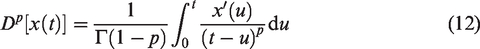
The third part of equation (9) is the fractional-order derivative. Different definitions are used for fractional-order derivatives, such as the Grünwald–Letnikov, Riemann–Liouville, and Caputo definitions.^26,27 They are all equivalent under certain conditions. Here Caputo’s definition is adopted with the form as

$$D^p\left[x\left(t\right)\right]=\frac{1}{\Gamma \left(1-p\right)}{\displaystyle {\int }_0^t\frac{x^{\text{′}}\left(u\right)}{{(t-u)}^p}\text{d}u}$$

(12)

where Γ(z) is Gamma function satisfying Γ(z + 1) = zΓ(z).

$${\dot{a}}_3=-\underset{T\to \infty }{\mathit{lim}}\frac{1}{T\omega }{\displaystyle {\int }_0^T{f}_3\left(a,\omega \right)\sin \varphi \text{d}\varphi =\underset{T\to \infty }{\mathit{lim}}\frac{1}{T\omega }}{\displaystyle {\int }_0^T-\epsilon k_4{D}^p\left[a\cos \varphi \right]\sin \varphi \text{d}\varphi }$$

(13a)

$${\dot{\theta }}_3=-\underset{T\to \infty }{\mathit{lim}}\frac{1}{T\omega }{\displaystyle {\int }_0^T{f}_3\left(a,\omega \right)\cos \varphi \mathrm{d}\varphi =\underset{T\to \infty }{\mathit{lim}}\frac{1}{T\omega }}{\displaystyle {\int }_0^T-\epsilon k_4{D}^p\left[a\cos \varphi \right]\cos \varphi \text{d}\varphi }$$

(13b)

In order to calculate the integrals, we introduce some important results about the definite integrals, which had been deduced in literature^15,16

$$\underset{T\to \infty }{\mathit{lim}}\frac{1}{T\omega }{\displaystyle {\int }_0^T\sin \varphi D^p\left[a\cos \varphi \right]\text{d}\varphi =-\frac{a{\omega }^{p-1}}{2}\sin \frac{p\pi }{2}}$$

(14a)

$$\underset{T\to \infty }{\mathit{lim}}\frac{1}{T\omega }{\displaystyle {\int }_0^T\cos \varphi D^p\left[a\cos \varphi \right]\text{d}\varphi =\frac{a{\omega }^{p-1}}{2}\cos \frac{p\pi }{2}}$$

(14b)

where 0 < p < 1. Substituting equation (14) into equation (13), it yields

$${\dot{a}}_3=-\underset{T\to \infty }{\mathit{lim}}\frac{1}{T\omega }{\displaystyle {\int }_0^T-\epsilon k_4{D}^p\left[a\cos \varphi \right]\sin \varphi \mathrm{d}\varphi =-\frac{1}{2}\epsilon a{k}_4{\omega }^{p-1}\sin \frac{p\pi }{2}}$$

(15a)

$$a{\dot{\theta }}_3=-\underset{T\to \infty }{\mathit{lim}}\frac{1}{T\omega }{\displaystyle {\int }_0^T-\epsilon k_4{D}^p\left[a\cos \varphi \right]\cos \varphi \mathrm{d}\varphi =\frac{1}{2}\epsilon a{k}_4{\omega }^{p-1}\cos \frac{p\pi }{2}}$$

(15b)

Substituting equations (10), (11), and (15) into equation (9), the following results are obtained

$$\dot{a}=-\frac{\epsilon }{2}\left(\frac{f\sin \theta }{\omega }+a\zeta +a{k}_4{\omega }^{p-1}\sin \frac{p\pi }{2}\right)$$

(16a)

$$\begin{array}{l}a\ge a_0\\ a\dot{\theta }=-\frac{1}{2\omega }\epsilon f\cos \theta -\frac{1}{2\omega }a\epsilon \delta +\frac{\epsilon k_3}{\pi \omega }\left(a{\varphi }_0-a_0\sin {\varphi }_0\right)+\frac{1}{2}\epsilon a{k}_4{\omega }^{p-1}\cos \frac{p\pi }{2}\end{array}$$

(16b)

$$\begin{array}{l}a<a_0\\ a\dot{\theta }=-\frac{1}{2\omega }\epsilon f\cos \theta -\frac{1}{2\omega }a\epsilon \delta +\frac{1}{2}\epsilon a{k}_4{\omega }^{p-1}\cos \frac{p\pi }{2}\end{array}$$

(16c)

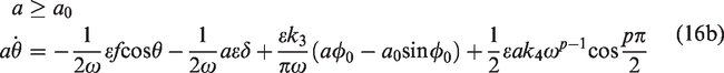
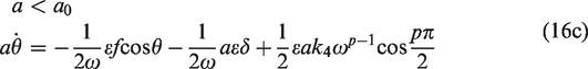
Substituting the original parameter into equation (16) yields

$$\dot{a}=-\frac{F\sin \theta }{2m\omega }-\frac{a}{2m}C\left(p\right)$$

(17a)

$$a\dot{\theta }=-\frac{F\cos \theta }{2m\omega }-\frac{\omega a}{2}+\frac{a}{2m\omega }K\left(p\right)$$

(17b)

where

$$C\left(p\right)=c+K_1{\omega }^{p-1}\sin \frac{p\pi }{2}$$

(18a)

$$K\left(p\right)=k_1+\frac{2k_2}{\pi }L\left(a\right)+K_1{\omega }^p\cos \frac{p\pi }{2}$$

(18b)

$$L\left(a\right)=\{\begin{array}{ll}{\varphi }_0-\frac{a_0}{a}\sin {\varphi }_0& a\ge a_0\\ 0& a<a_0\end{array}$$

(19)

C(p) and K(p) are defined as the equivalent linear stiffness coefficient and equivalent linear damping coefficient of the system, respectively.^12–16 Equation (17) indicates that both the piecewise linear term and the fractional-order term are crucial in equation (1). Accordingly, the parameters in the two terms, that is, the piecewise parameters a₀ and k₂, the fractional coefficient K₁, and the fractional order p are all important in system dynamics. The piecewise stiffness k₂ and clearance a₀ are directly related to the stiffness of system. The fractional-order parameters influence not only the system stiffness but also the system damping. The following conclusions can be obtained from equation (18). When p is close to zero, the fractional-order differential item acts almost as the system stiffness. As p increases gradually, the fractional-order differential item affects not only system stiffness but also system damping. When p is close to 1, the fractional-order differential item will behave only as system damping.

Steady-state solutions and their stability conditions

Steady-state solutions

For nonlinear systems, the steady-state response $\left(\overline{a},\overline{\theta }\right)$ of the system is much more important and meaningful. Assume that $\dot{a}=0$ and $\dot{\theta }=0$ ; equation (20) can be obtained as

$$-\frac{\mathit{F}\sin \overline{\theta }}{2m\omega }-\frac{\overline{a}}{2m}C\left(p\right)=0$$

(20a)

$$-\frac{\mathit{F}\cos \overline{\theta }}{2m\omega }-\frac{\omega \overline{a}}{2}+\frac{\overline{a}}{2m\omega }K\left(p\right)=0$$

(20b)

After the elimination of $\overline{\theta }$ from equation (20), the amplitude–frequency equation can be obtained as

$${\overline{a}}^2\left\{{\omega }^2{C}^2\left(p\right)+{\left[m{\omega }^2-K\left(p\right)\right]}^2\right\}=F^2$$

(21)

Letting $s=\frac{\omega }{{\omega }_0}$ and $F=a_0^{\hspace{0.17em}}{\omega }_0^{2}A$ , equation (20) can be obtained as

$$a^2\left\{s^2\frac{m{C}^2\left(p\right)}{k_1}+m^2{\left[s^2-\frac{K\left(p\right)}{k_1}\right]}^2\right\}=A^2$$

(22)

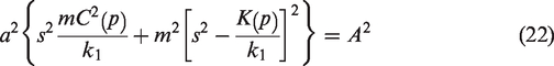
Obviously, equation (22) is an implicit about amplitude a, and it is difficult to directly solve it. In this paper, Matlab’s fsolve command is used to solve the problem, and it is obtained in a segmented way, that is, w is taken as a variable to select different segmented intervals, in which the curves in each segment are guaranteed to be monotonous, and different initial values need to be selected for different interval segments, so that the whole amplitude–frequency curve can be obtained by connecting each segment of curves.

Stability conditions

To analyze the stability of the stationary solution, we substitute $a=\overline{a}+\Delta a$ and $\theta =\overline{\theta }+\Delta \theta$ into equation (17), where $\Delta a$ and $\Delta \theta$ are two small perturbations. Then

$$\frac{d\Delta a}{\mathit{dt}}=-\frac{C\left(p\right)}{2m}\Delta a-\frac{\mathit{F}\cos \overline{\theta }}{2m\omega }\Delta \theta$$

(23a)

$$\frac{d\theta }{\mathit{dt}}=\left[\frac{\mathit{F}\cos \overline{\theta }}{2m{\overline{a}}^2\omega }+\frac{k_2}{\pi m\omega }{L}_{\Delta a}\left(\overline{a}\right)\right]\Delta a+\frac{\mathit{F}\sin \overline{\theta }}{2m\overline{a}\omega }\Delta \theta$$

(23b)

where

$$L_{\Delta a}\left(\overline{a}\right)=\{\begin{array}{ll}\frac{2a_0\sqrt{1-\frac{a_0^2}{{\overline{a}}^2}}}{{\overline{a}}^2}& \overline{a}\ge a_0\\ 0& \overline{a}<a_0\end{array}$$

Based on equations (20) and (23), one could obtain the characteristic determinant of the system

$$\det \left[\begin{array}{cc}-\frac{C\left(p\right)}{2m}-\lambda & \frac{\omega \overline{a}}{2}-\frac{\overline{a}}{2m\omega }K\left(p\right)\\ \frac{\omega }{2\overline{a}}-\frac{K\left(p\right)}{2m\omega \overline{a}}+\frac{k_2{L}_{\Delta a}\left(\overline{a}\right)}{\pi m\omega }& -\frac{C\left(p\right)}{2m}-\lambda \end{array}\right]=0$$

(24)

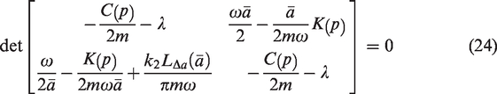
We can analyze its stability condition for two cases:

$a\ge a_0$ . Using equation (24), we get the characteristic equation as

$${\lambda }^2+\frac{C\left(p\right)}{m}\lambda +\frac{C^2\left(p\right)}{4m^2}+Z^2-\frac{k_{2}Z{L}_{\Delta a}\left(\overline{a}\right)}{\pi m\omega }=0$$

(25)

where $\text{Z}=\frac{\omega }{2}-\frac{K(p)}{2mw}$ .

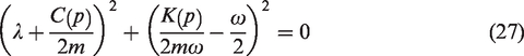
Furthermore, the stability condition for the steady-state solution of $a\ge a_0$ could be established as

$$H=\frac{C^2\left(p\right)}{4m^2}+Z^2-\frac{k_{2}Z{L}_{\Delta a}\left(\overline{a}\right)}{\pi m\omega }\ge 0$$

(26)

Figure 2 shows the amplitude–frequency curve and its stability conditions for the steady-state solution. The stability condition curve is denoted by a solid blue line, which is the boundary between the unstable and stable regions. The region above the curve, that is, $H>0$ , is an asymptotically stable region. Therefore, segment AB is a stable solution. However, point A of the intersection of the two curves, that is, $H=0$ , is a stable point. The region below the curve, that is, $H<0$ , is the unstable region. Therefore, segment AC of the amplitude–frequency curve is the unstable one. Jumping phenomenon will occur when the amplitude–frequency curve of the system passes through the unstable region. The unstable region should be avoided or reduced when designing a system. The influence of system parameters on unstable regions is discussed in a subsequent section.

Figure 2.

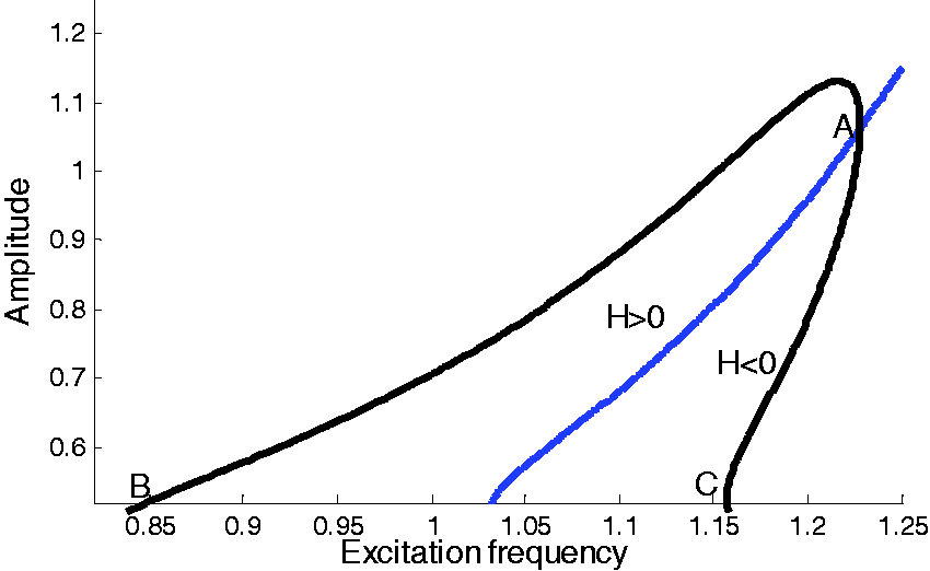
Amplitude–frequency curve and its stability conditions for the steady-state solution ( $a\ge a_0$ ; m = 10, c = 1, F = 3, k₁ = 10, k₂ = 10, a₀ = 0.5, K₁ = 0.4, and p = 0.5).

• 2.  $a<a_0$ , according to equation (24) one can get

  $${\left(\lambda +\frac{C\left(p\right)}{2m}\right)}^2+{\left(\frac{K\left(p\right)}{2m\omega }-\frac{\omega }{2}\right)}^2=0$$

  (27)

The characteristic roots can be obtained as

$${\lambda }_{1,2}=-\frac{C\left(p\right)}{2m}\pm i\left(\frac{K\left(p\right)}{2m\omega }-\frac{\omega }{2}\right)$$

(28)

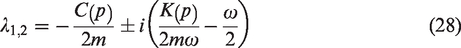
According to the above analysis, we know that the real parts of the eigenvalues are less than zero, so that the solution for $a<a_0$ is stable.

Numerical simulations

Comparisons between analytical and numerical results

To validate the approximate approaches, the periodic solutions obtained by the averaging method are compared with the solutions from the numerical integration method. The numerical method uses the series expanding technique described in literature^26,27 and equation (29) is the approximate formula of the method

$$D^p\left[x\left(t_l\right)\right]\approx h^{-p}{\displaystyle \sum }_{j=0}^l{C}_j^{p}x\left(t_{l-j}\right)$$

(29a)

$$C_j^p=\left(1-\frac{1+p}{j}\right)C_{j-1}^p$$

(29b)

where $C_j^p$ is the binomial coefficient of the fractional-order item, $C_0^p=1$ , $t_l^{\hspace{0.17em}}$ is the sample point( $t_l^{\hspace{0.17em}}=\mathit{lh}$ ), and h is the time step.

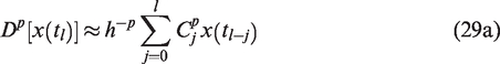
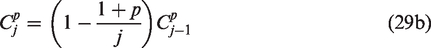
As an example, the basic parameters of the system are given by m = 10, c = 1, F = 3, k₁ = 10, k₂ = 12, a₀ = 0.7, K₁ = 0.1, and p = 0.5. The solid line in Figure 3 shows the amplitude of the stable periodic solution. The circles in Figure 3 represent the result of the numerical simulation, and the time step is taken at h = 0.004. The approximate and numerical solutions are in excellent agreement in the cases of primary resonance, and jumping phenomenon occurs at points A and B (a₀ = 0.7).

Figure 3.

Comparison of the amplitude–frequency curve by analytical and numerical methods (m = 10, c = 1, F = 3, k₁ = 10, k₂ = 12, a₀ = 0.7, K₁ = 0.1, and p = 0.5).

Effects of piecewise linear parameters on system dynamics

The following section presents the study about the effects of the two parameters of the piecewise linear term on the system dynamics.

Clearance a₀

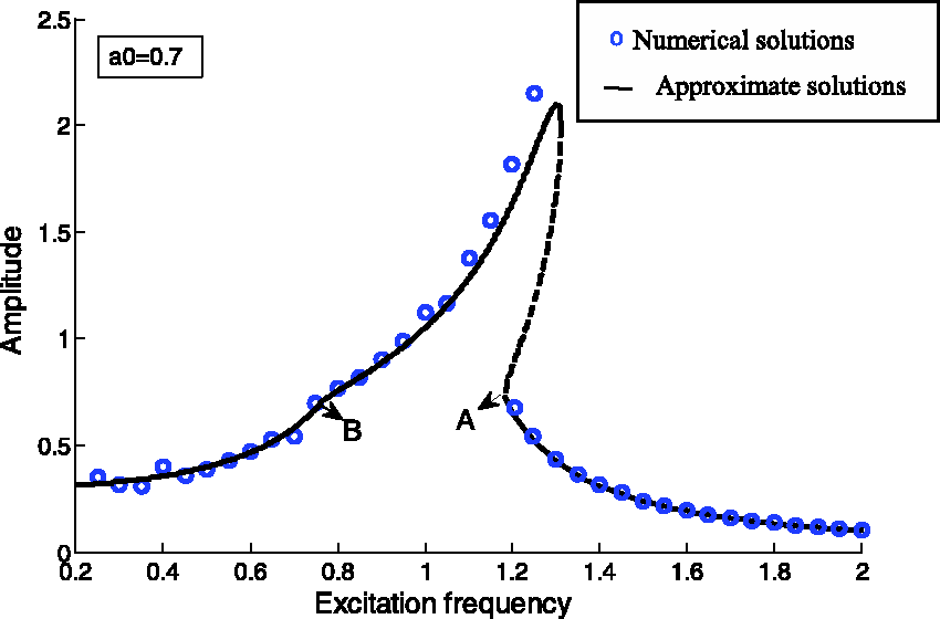
With other system parameters remaining unchanged, three clearance parameters, a₀ = 0.5, a₀ = 0.7, and a₀ = 0.9, are selected to investigate the different dynamic response modes, and the amplitude–frequency curves are obtained in Figure 4. The jump points of the amplitude–frequency curves appear where a₀ is 0.5, 0.7, and 0.9. The curves below the jump points are coincidental because the other parameters remain unchanged.

Figure 4.

Effects of clearance a₀ on the amplitude–frequency curves.

It can be seen from equation (18b) that with the increase of a₀, the equivalent linear stiffness coefficient will decrease. The increase of the clearance a₀ can contribute to smaller resonant frequency of response. But, as shown in equation (18a), the larger the clearance a₀, the equivalent linear damping coefficient of the system will not change. Accordingly, as shown in Figure 4, with the increase of a₀, the resonant amplitude increases slightly. At the same time, the larger the clearance a₀ leads to the larger of the unstable region of the system.

Piecewise stiffness k₂

Similarly, the influence of the stiffness k₂ of spring b on the dynamic behavior is analyzed as the other system parameters remain unchanged. Three stiffness parameters, that is, k₂ = 10, k₂ = 15, and k₂ = 20, are selected to investigate the different dynamic response modes based on the amplitude–frequency in equation (22), and the different amplitude–frequency curves of steady-state solution are shown in Figure 5. When k₂ increases gradually, the jumping point of the system amplitude–frequency curves keeps invariable because clearance a₀ is the same. However, the nonlinearity of the system ω will increase gradually in this procedure. Furthermore, with the k₂ increases gradually, the resonance curves continuously shift to the direction of frequency value increase, and the resonance amplitude decreases. Moreover, the unstable region increases slightly as k₂ increases. Therefore, the piecewise stiffness k₂ affects not only the resonant amplitude and frequency of the system but also the size of the unstable region.

Figure 5.

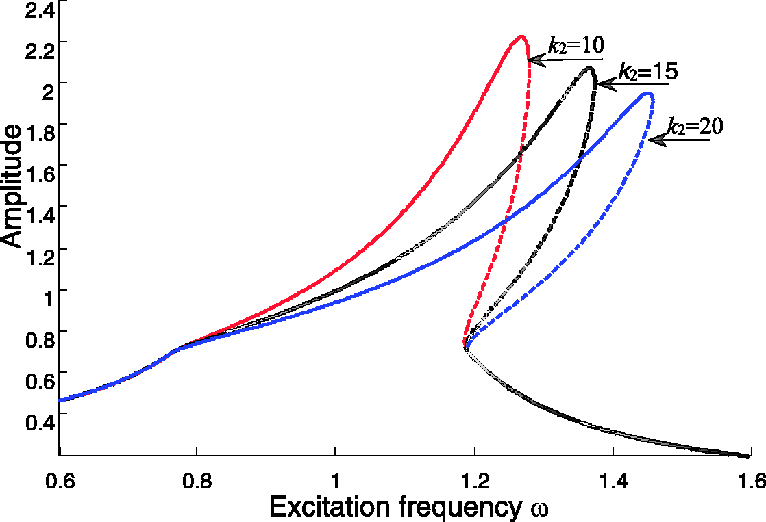
Effects of the stiffness k₂ on the amplitude–frequency curves.

Effects of fractional-order term on system dynamics

Next, the effects of fractional-order coefficient K₁ and order p on system dynamics are studied.

Fractional-order coefficient K₁

The amplitude–frequency curves with different fractional-order coefficients K₁ as 0.3, 0.6, and 0.9 are shown in Figure 6. When fractional-order coefficient K₁ increases gradually, the equivalent linear damping and equivalent linear stiffness of the system will increase simultaneously based on equations (18a) and (18b). This effect lowers both the resonance amplitude and resonance frequency of the system and reduces the unstable region and the frequency range of the resonance region.

Figure 6.

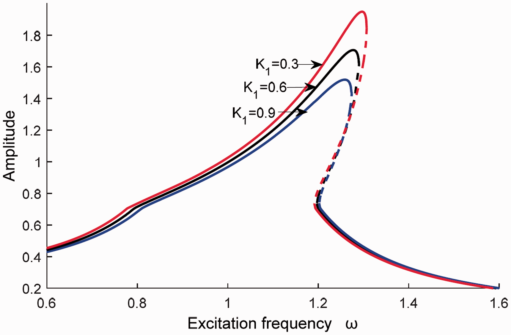
Effects of the fractional-order coefficient K₁ on the amplitude–frequency curves.

Fractional order p. Four fractional order parameters, that is, p = 0, p = 0.1, p = 0.3, p = 0.6, and p = 0.9 and p = 1 are selected to study the different dynamic response modes, and the results are shown in Figures 7 and 8. As shown in equation (18a), the larger the fractional order p, the larger the equivalent linear damping of the system. As shown in Figure 6, the resonance amplitude of the system will become smaller with the increase of fractional order. Furthermore, the larger the fractional order p, the smaller the equivalent linear stiffness of the system, which will result in a smaller resonant frequency. Given that the parameters of the piecewise linear term do not change, the amplitude–frequency curves of the system do not shift. Meanwhile, with the increase of p, the frequency range of the resonance region becomes noticeably smaller, and the size of the unstable region also becomes smaller. Therefore, the fractional-order order p affects not only the resonance amplitude and the resonant frequency of the system but also the frequency range of the resonance region and the size of the unstable region.

Figure 7.

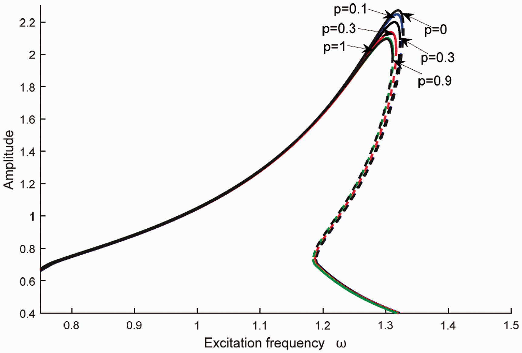
Effects of the fractional-order order p on the amplitude–frequency curves.

Figure 8.

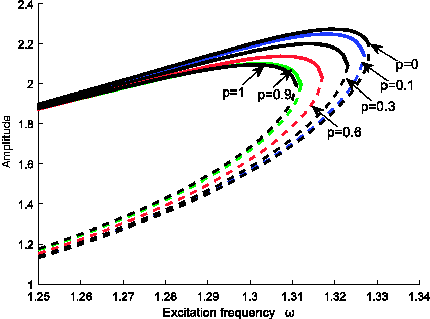
Effects of the fractional-order order p on the amplitude–frequency curves.

Conclusions

In this study, a piecewise linear SDOF oscillator with fractional-order derivative is analyzed by the averaging method, and the approximately analytical solution associated with the amplitude–frequency curves are obtained. Then, the amplitude–frequency equations are used for stability analysis, and the stability condition is established. The numerical results are also obtained by simulations, and the coincidence is good. Finally, the effects of the system parameters on the dynamic behaviors are studied. Clearance a₀, piecewise stiffness k₂, fractional-order coefficient K₁, and fractional-order order p affect not only the unstable region but also the resonant amplitude and resonant frequency of the system. In addition, the fractional-order coefficient K₁ and the fractional-order order p influence the frequency range of the resonance region of the system. Therefore, the fractional-order term and the piecewise linear term both play an important role in the dynamic behavior of the system. These results could present useful reference to analyze the dynamic behavior for similar piecewise linear with fractional-order derivative systems.