Investigation on the transient response of a speed-varying rotor with sudden unbalance and its application in the unbalance identification

Abstract

It is well known that the sudden unbalance is harmful for rotor systems, since it is in huge amount and has a strong impact. Thus, it is difficult to identify the unbalance from the sudden unbalance response of rotor and very few studies have been done on this topic. This paper focuses on the transient response characteristics of the speed-varying rotor when the sudden unbalance occurs, and the inherent correlation between the unbalance and the transient characteristic quantity. First, different time-dependent functions modelling the loading process of sudden unbalance are derived and compared with the experiment results of the test rotor. The selection principles of function type and duration value are presented. Analyses of transient response characteristics are conducted over the run-up process of the rotor with different parameters of sudden unbalance. Variations of transient response characteristics are summarized into three forms. The varying laws and interrelations of characteristic quantities, and the corresponding parameter region of sudden unbalance are illustrated for each form. Based on the transient analysis results, the momentary positions and angular variations of the rotor disc at some key time instants are illustrated via introducing the key-phase signal. A novel transient-vibration-based method for unbalance identification is proposed. Only a single run-up measurement is required. Numerical experiments verify the effectiveness of the method. In summary, the proposed method can provide a new way for the unbalance identification using the transient response.

Introduction

Unbalance is one of the most common faults existing in rotating machinery. ¹ The rotating unbalance can be categorized into initial unbalance and sudden unbalance based on the form of generation. The initial unbalance arises due to some reasons such as porosity in casting, non-uniform density of material and manufacturing tolerance, ² while the sudden unbalance is generally caused by gain or loss of material during operation. ³ Both of them can cause undesirable vibrations which may lead to bearing failure, incipient cracks and noise.^4,5

During the past decades, a significant amount of researches have been done on the dynamical response of rotor system excited by sudden unbalance load. One relevant topic is the amplitude of the transient displacement and the impact load generated. Genta, ⁶ Kailinowski et al., ⁷ Dzenan, ⁸ Wang et al., ⁹ and Yu et al., ¹⁰ established dynamic equations to study the transient response caused by sudden unbalance. The effects of different parameters, such as excitation amplitude, internal damping, gyroscopic moment and support stiffness on the transient vibrations were investigated. Meanwhile, a few sudden unbalance experiments were carried out to verify the theoretical results.^11–14 Existing works demonstrated that the sudden unbalance can lead to amplification of vibration response instantaneously. The transient displacement and impact load are related to the operating state and low-order natural frequencies exist in the frequency domain. Another topic of interest is the nonlinear dynamical response due to sudden unbalance, suppression effects of the damping structure on the transient vibration and numerical calculation methods for the transient response.^15–24 Ma et al. ²⁵ analyzed the dynamic characteristics of rotor system under different rubbing forms caused by sudden unbalance excitation. Zhou et al. ²⁶ compared the performance of different floating ring squeeze film dampers in controlling the transient response of sudden unbalance. Wang et al. ²⁷ presented a design of safety structure named “fusing” and analyzed its effectiveness in reducing the vibration amplitude, as well as possible dynamic problems which may be introduced.

In above studies, the rotor system is usually set operating in a constant rotational speed condition. At present, few investigations have focused on the sudden unbalance response characteristics of the speed-varying rotor system. Except for the radial centrifugal load generated by unbalance moment, the tangential inertial load caused by the angular acceleration is also present in the speed-varying process. Furthermore, the unbalance load and the gyroscopic moment are time-varying quantities, which make the load variation of rotor system more complex. Lawrence et al. ²⁸ studied the transient response of rotor system subject to blade loss with asymmetric rotational inertia during deceleration and analyzed the influence of deceleration time on the peak value of vibration response. Braut et al. ²⁹ established the rotor-stator model with a shaft bow and investigated the contact vibration response in a run-down due to the emergency shutdown caused by sudden unbalance. In practice, sudden unbalance can also occur in the start-up procedure of a machine. Grapis et al. ³⁰ analyzed the rotor-stator collision, the full annular rub and the high dynamic load of an overcritical high-speed rotor due to a rapid increase of unbalance. Torkhani et al. ³¹ investigated light, medium and heavy partial rubs, respectively, during speed transients of rotating machines via numerical simulation and experimental observation. Their research focused more on the nonlinear rub-impact response of the rotor. As can be seen, there is no detailed study on the sudden unbalance response characteristics of rotor system during acceleration process without contact and rub. Furthermore, to model the sudden unbalance accurately, the time-dependent function which can express the loading process of sudden unbalance load needs a systematic and experimental investigation. ³²

Initial unbalance identification in the rotor system is critical for rotor balancing. ³³ There are two classical methods,^34,35 namely the modal balancing method and the influence coefficient balancing method. The implementation of the two methods usually requires the measurements of the steady-state response data at some selected rotational speeds and a number of test runs, which is costly and time-consuming. Therefore, the trend in the unbalance identification is to reduce the number of test runs and measurements required.

Instead of the steady-state response data, some scholars hope to use the response data collected in the transient operation process to identify the rotor unbalance. Until recently, a few studies have been conducted in this area. Some researchers identified and diagnosed rotor unbalance using measured vibration response from a single machine run-down.^36–38 Shamsah ³⁹ proposed a method for estimating rotor unbalance from a single run-up using reduced sensors. Their method is model-based which requires an accurate numerical model of the machine. Huang ⁴⁰ used the modal unbalance angle and the equivalent modal unbalance magnitude to express the modal unbalance, and identified the modal unbalance angle by using the accelerating response information. The modal unbalance magnitude was calculated with trial runs. Wen ⁴¹ extracted rotating frequency vibration information near the critical speed from the run up accelerating response data, and obtained the initial phase by introducing the key phase signal. The correction masses were calculated by adding appropriate trial weights in trial runs. Their method is vibration-based and the results show that the number of test runs and the measurements required can be reduced effectively compared with the traditional balancing method. However, the method still needs at least one test run to calculate the unbalance magnitude.

To obtain more vibration information during a single run-up to identify the rotor unbalance, the transient external excitation was applied to the rotor during the transient operation. Iida ⁴² conducted an experiment to identify the residual unbalance of the rotor-bearing system by applying impulse excitation. Tiwari and Chakravarthy ⁴³ proposed an identification algorithm for the estimation of the residual unbalance based on the impulse response measurements in a rotor-bearing system. Lou et al. ⁴⁴ used an active magnetic executor to apply external excitation and identify the rotor unbalance. However, those procedures need a high-power exciter which is difficult to implement in the transient operation and may produce a damage to the rotor. If trial weights are added to the rotor during run-up operation by the way of sudden unbalance, then it can be considered as an effective transient external excitation. The procedure of measuring the initial accelerating response, installing trial weights and measuring the accelerating response after installation can be replaced by a new one, which includes measuring the initial accelerating response and measuring the sudden unbalance response caused by the trial weight loss during the same run-up operation. In that way, one test run can be reduced. This method can also inherit the advantage of the trial weight excitation, which is reliable, accurate and easy-to-apply. To the author’s best knowledge, no relevant research has been seen on publication yet.

This paper has two research objectives. The first one is to conduct a detailed study on the sudden unbalance response characteristics of rotor system during acceleration process without contact and rub. The dynamic modelling and model validation are carried out. The second one is to determine the relationships between rotor unbalance and characteristic quantities, and to propose a method of identifying the initial rotor unbalance parameters by using the sudden unbalance response.

The rest of this paper is organized as follows. In the Mathematical modeling section, the finite element (FE) model of the test rotor is built. In the Model validation section, validation experiments for the FE model and the time-dependent function of sudden unbalance are carried out. In the Transient response characteristics of sudden unbalance for a speed-varying rotor section, characteristic quantities of the sudden unbalance response and the varying laws are described. In the Identification of initial unbalance based on the transient response data of sudden unbalance section, the relationship between the rotor unbalance and the characteristic quantities of the sudden unbalance response is determined and the identifying method of initial unbalance is proposed. In the Identification results and discussions section, numerical experiments are carried out to validate the identifying method. The Conclusion section draws the main conclusions.

Mathematical modeling

The FE model of the rotor-bearing system used in this study is shown in Figure 1, which also represents the test rotor whose details are presented in the model validation section. The shaft is modeled by the finite beam element consists of two nodes with four degrees-of-freedom each (two translational and two rotational).^45,46 The disk is modeled as a rigid mass with gyroscopic moments added to the damping matrix. The bearings are modeled as a combination of stiffness and damping at the corresponding nodes in the FE model. Thus, the equation of motion for the rotor-bearing system can be expressed as

$$\mathit{M}\ddot{q}\left(t\right)+\mathit{D}\ddot{q}\left(t\right)+\mathit{K}\mathit{q}\left(t\right)=\mathit{F}\left(t\right)$$

(1)

where M is the mass matrix, K is the stiffness matrix including bearing stiffness, D is the damping matrix including bearing damping and gyroscopic effects and q (t) is the nodal displacement vector. The force vector F (t) consists of the initial unbalance force F _i (t) and the sudden unbalance force F _s (t).

Figure 1.

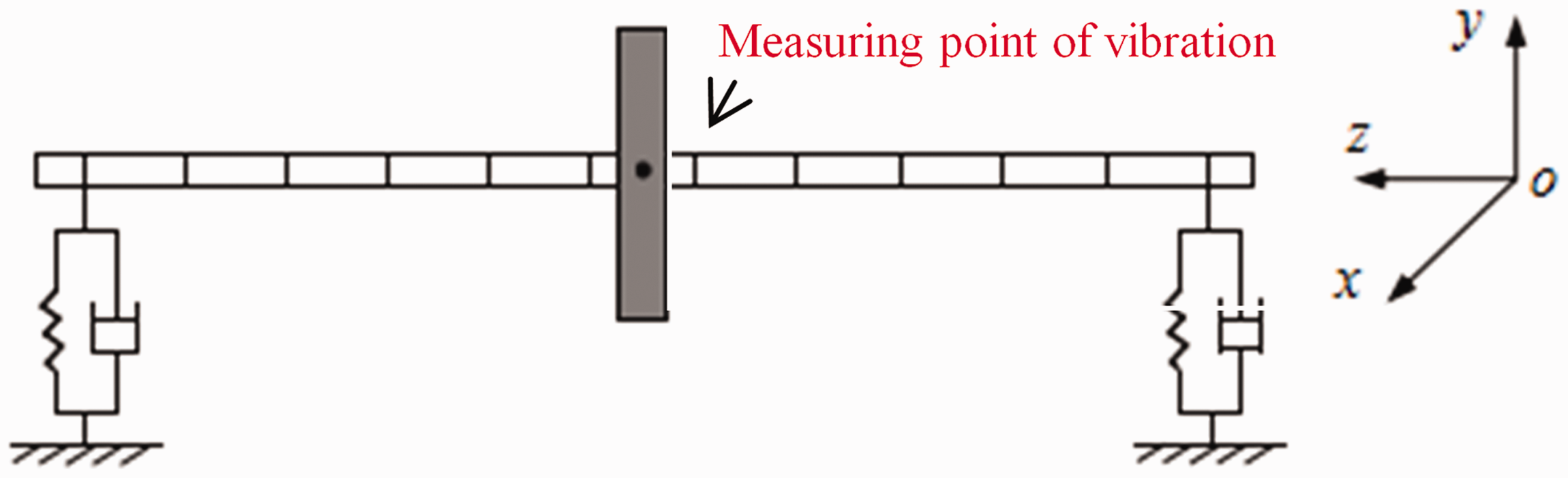
FE model of the test rotor. (a) Test rotor; (b) sensors of x and y (c) rotor disc.

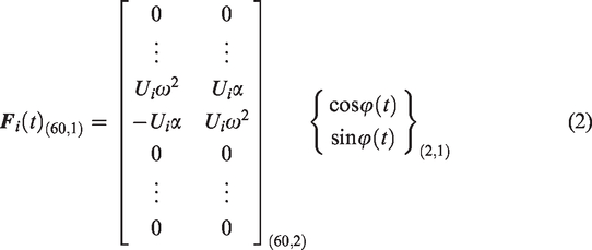
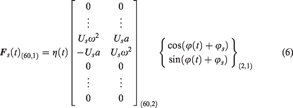
Both the initial unbalance force and the sudden unbalance force are exerted on the disk of rotor, since the disk is considered as the source of unbalance. They can be given by

$${\mathit{F}}_i{\left(t\right)}_{\left(60,1\right)}={\left[\begin{array}{cc}0& 0\\ ⋮& ⋮\\ U_i{\omega }^2& U_i\alpha \\ -U_i\alpha & U_i{\omega }^2\\ 0& 0\\ ⋮& ⋮\\ 0& 0\end{array}\right]}_{\left(60,2\right)}{\left\{\begin{array}{c}\cos \phi (t)\\ \sin \phi (t)\end{array}\right\}}_{\left(2,1\right)}$$

(2)

where U_i is the initial unbalance moment, ω is the rotation angular velocity, ɑ is the angular acceleration and φ(t) is the rotation angle.

For the steady-state case, the rotation angle φ(t) is given by

$$\phi \left(t\right)=\omega t+{\phi }_i$$

(3)

For the transient-state case, the rotation angular velocity ω and the rotation angle φ(t) could be given by

$$\omega ={\omega }_0+at$$

(4)

$$\phi \left(t\right)={\omega }_{0}t+\text{1}/\text{2}\left(a{t}^{\text{2}}\right)+{\phi }_i$$

(5)

where ω₀ is the initial rotation angular velocity and φ_i is the phase angle of initial unbalance. Then equation (2) takes the form as follows

$${\mathit{F}}_s{\left(t\right)}_{\left(60,1\right)}=\eta \left(t\right){\left[\begin{array}{cc}0& 0\\ ⋮& ⋮\\ U_s{\omega }^2& U_{s}a\\ -U_{s}a& U_s{\omega }^2\\ 0& 0\\ ⋮& ⋮\\ 0& 0\end{array}\right]}_{\left(60,2\right)}{\left\{\begin{array}{c}\cos \left(\phi (t)+{\phi }_s\right)\\ \sin \left(\phi (t)+{\phi }_s\right)\end{array}\right\}}_{\left(2,1\right)}$$

(6)

where U_s is the sudden unbalance moment, φ_s is the phase angle of sudden unbalance relative to initial unbalance and η(t) is a time-dependent function which represents the loading process of sudden unbalance load.

Model validation

Description of the test rotor

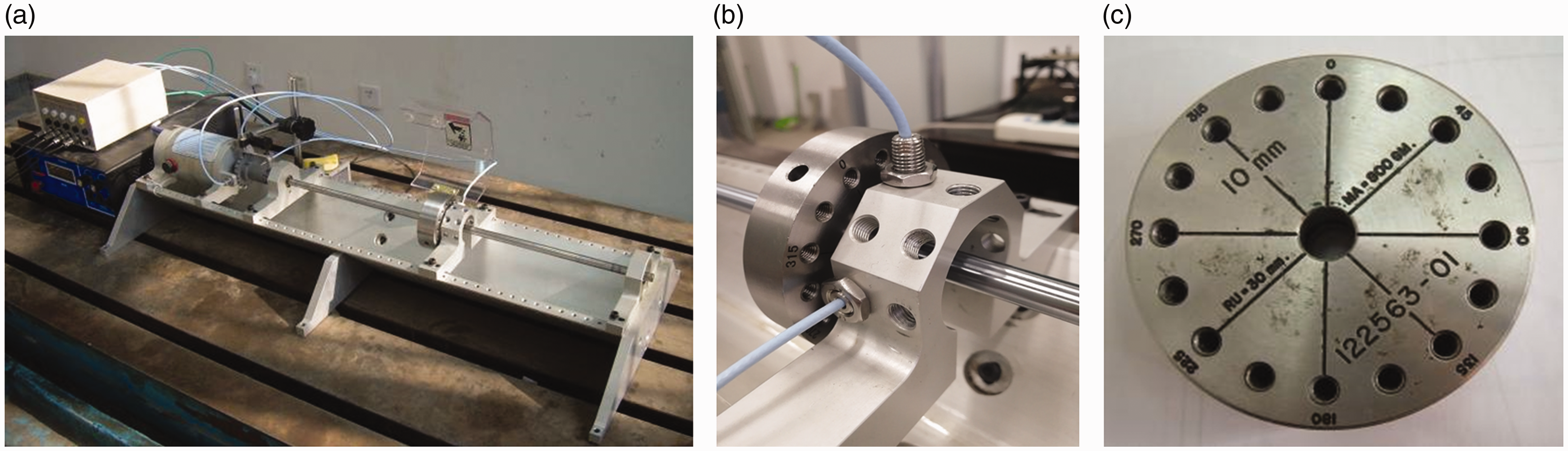
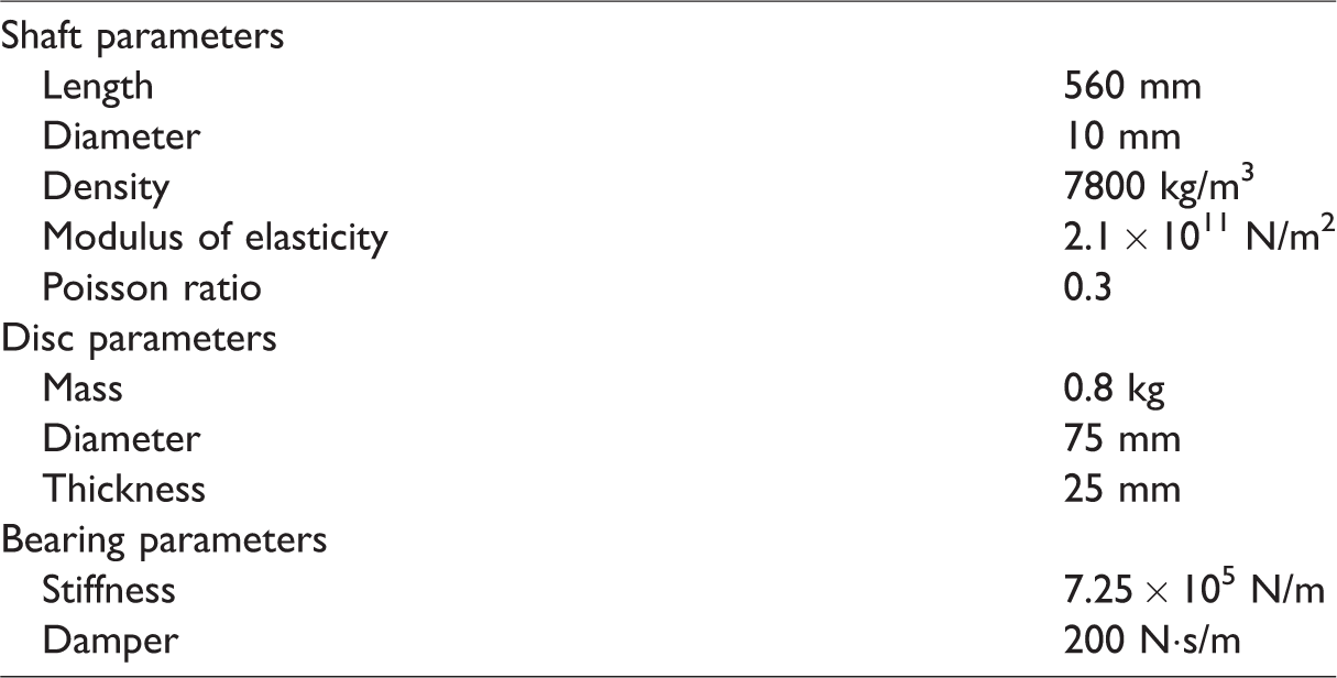
The test rotor is shown in Figure 2(a). It is supported on two bush bearings, and driven by an AC electric motor with the maximum speed of 10,000 r/min. The shaft is connected to the motor by a flexible coupling. The vibration displacements of the rotor are monitored by two eddy current displacement sensors, as shown in Figure 2(b). The disk has 16 holes spaced 22.5° from each other, and the radial distance d from the center of holes to the shaft center-line is 30 mm, as shown in Figure 2(c). The unbalance mass m is placed at one specific hole in which the phase angle of unbalance can be determined directly. The unbalance moment U can be given by multiplying m and d. The main parameters of the test rotor are listed in Table 1.

Figure 2.

Experimental set-up. (a) Run-up response; (b) FFT.

Table 1.

Rotor system parameters.

Shaft parameters
Length	560 mm
Diameter	10 mm
Density	7800 kg/m3
Modulus of elasticity	2.1 × 1011 N/m2
Poisson ratio	0.3
Disc parameters
Mass	0.8 kg
Diameter	75 mm
Thickness	25 mm
Bearing parameters
Stiffness	7.25 × 105 N/m
Damper	200 N·s/m

Validation of FE model

The practical rotor disk was initially balanced first, then an unbalance mass of 0.4 g was placed in the hole at 0° to generate an unbalance moment of 12 g·mm. The rotor was run and the run-up response was measured. The simulated response calculated by the FE model is compared with the measured experiment response to check its accuracy, as shown in Figure 3(a), while the spectrum comparison is shown in Figure 3(b). It can be seen that the simulated curves agree well with the experimental curves. The critical speed calculated is 1680 r/min for the FE model, while the practical critical speed is 1688 r/min. The relative error is only 0.42%, which proved the accuracy of rotor FE model.

Figure 3.

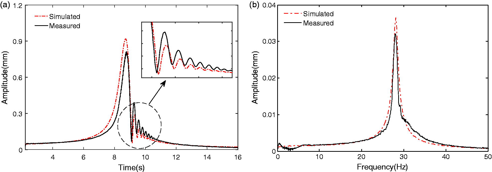
Comparisons of simulated response and measured response. (a) Installation diagram; (b) equivalence test.

Time-dependent function of sudden unbalance

In most studies, the sudden unbalance was considered as an instantly completed process so that the sudden unbalance load is modeled by a unit step function. Some researchers considered the sudden unbalance as a continuous process and use the continuous function to express the loading process, such as the cycloidal front function ⁴⁷ and the infinitely differentiable real function. ⁴⁸ However, the systematic experimental investigation and simulation study are still needed on the following points, i.e. the difference between the measured response and the simulated response using unit step function and continuous function, respectively, the influencing factors on the duration of sudden unbalance process and the applicability of the unit step function and the continuous function. These are also the main concerns in this section.

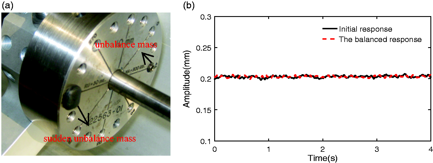
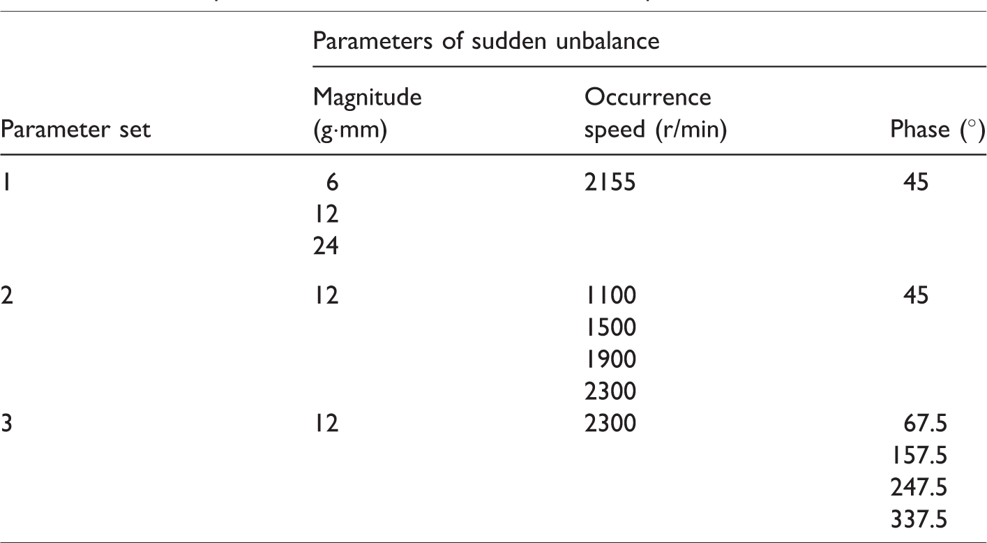
In experiment, an unbalance mass and a sudden unbalance mass were added diametrically opposite each other about the disk center as shown in Figure 4(a), then the rotor was driven to run, and the balanced response of rotor was checked to ensure that the two unbalance moments are equal, as shown in Figure 4(b). When the rotor ran to a predetermined speed, the sudden unbalance mass will be released due to centrifugal force. At this instant, the unbalance mass will generate a sudden load to the rotor system. Three groups of experiments were conducted respectively to analyze the influences of different parameters of sudden unbalance to the transient response, i.e. the magnitude, the occurrence speed and phase. The experimental parameter sets are listed in Table 2.

Figure 4.

Simulation diagram of sudden unbalance. (a) 6 g·mm; (b) 12 g·mm and (c) 24 g·mm.

Table 2.

Different parameter sets for sudden unbalance experiments.

Parameter set	Parameters of sudden unbalance
	Magnitude (g·mm)	Occurrence speed (r/min)	Phase (°)
1	6	2155	45
	12
	24
2	12	1100	45
		1500
		1900
		2300
3	12	2300	67.5
			157.5
			247.5
			337.5

Meanwhile, three types of time-dependent functions used in the numerical simulation are given as follows:

Unit step function

$$\eta \left(t\right)=\{\begin{array}{c}0,t<t_{\mathit{start}}\\ 1,t\ge t_{\mathit{start}}\end{array}$$

(7)

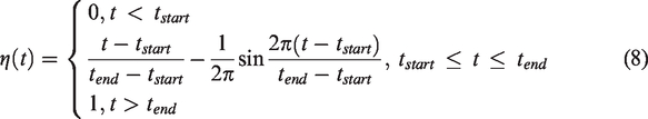
Cycloidal front function

$$\eta \left(t\right)=\{\begin{array}{l}0,t<t_{\mathit{start}}\hfill \\ \frac{t-t_{\mathit{start}}}{t_{\mathit{end}}-t_{\mathit{start}}}-\frac{1}{2\pi }\sin \frac{2\pi \left(t-t_{\mathit{start}}\right)}{t_{\mathit{end}}-t_{\mathit{start}}},t_{\mathit{start}}\le t\le t_{\mathit{end}}\hfill \\ 1,t>t_{\mathit{end}}\hfill \end{array}$$

(8)

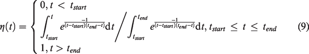
Infinitely differentiable real function

$$\eta \left(t\right)=\{\begin{array}{l}0,t<t_{\mathit{start}}\hfill \\ {\displaystyle {\int }_{t_{\mathit{start}}}^t{e}^{\frac{-1}{(t-t_{\mathit{start}})(t_{\mathit{end}}-t)}}}\text{d}t/{\displaystyle {\int }_{t_{\mathit{start}}}^{t_{\mathit{end}}}{e}^{\frac{-1}{(t-t_{\mathit{start}})(t_{\mathit{end}}-t)}}}\text{d}t,t_{\mathit{start}}\le t\le t_{\mathit{end}}\hfill \\ 1,t>t_{\mathit{end}}\hfill \end{array}$$

(9)

where t_start represents the start time of sudden unbalance and its value can be identified from the mutation point of the measured response of sudden unbalance. t_end represents the end time of sudden unbalance, so the duration of the loading process can be expressed by (t_end-t_start). Once the value of t_start is determined, we can give and adjust the duration value until the fluctuation period of simulated transient response curve is consistent with the measured transient response curve. For convenience, we take t_start as the zero point of the time coordinate axis.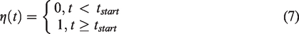

The parameters of sudden unbalance used in the simulations are exactly the same as those in Table 2. Figures 5 to 7 show the comparison results between the simulated responses and the measured responses, obtained by different parameters of sudden unbalance, respectively. The value of (t_end-t_start) selected are marked on each figure.

Figure 5.

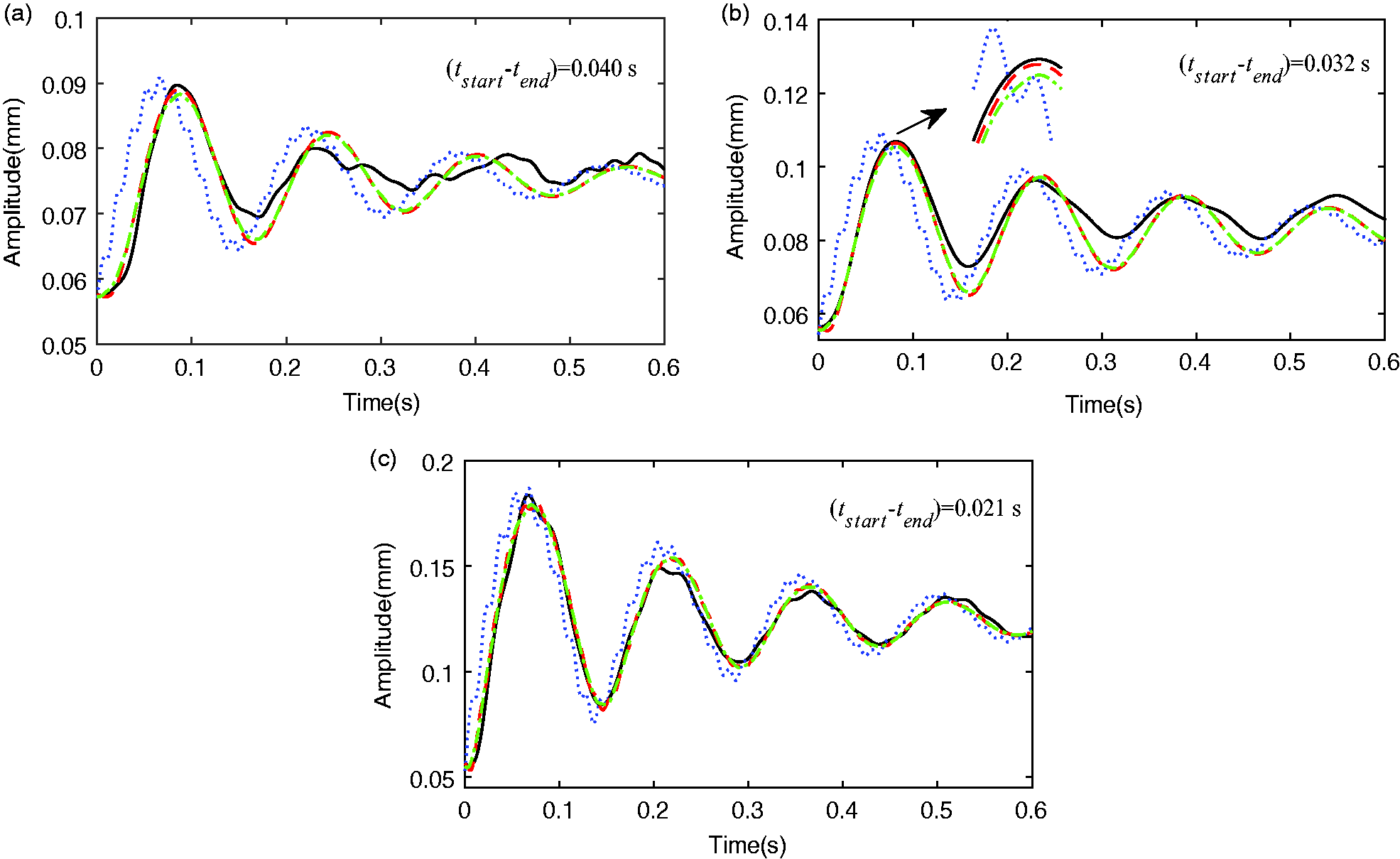
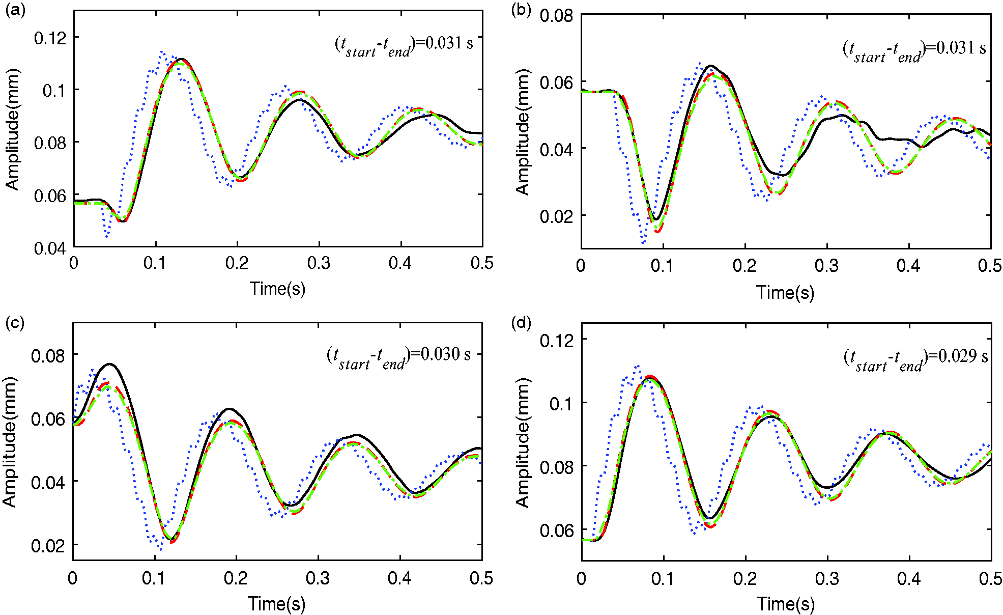
The comparison of transient response with different unbalance magnitudes, the measured response (solid line), the simulated response with Unit step function (dotted line), the simulated response with Cycloidal front function (dashed line) and simulated response with Infinitely differentiable real function (dot-dash line). (a) 1100 r/min; (b) 1500 r/min; (c) 1900 r/min; (d) 2300 r/min.

Figure 6.

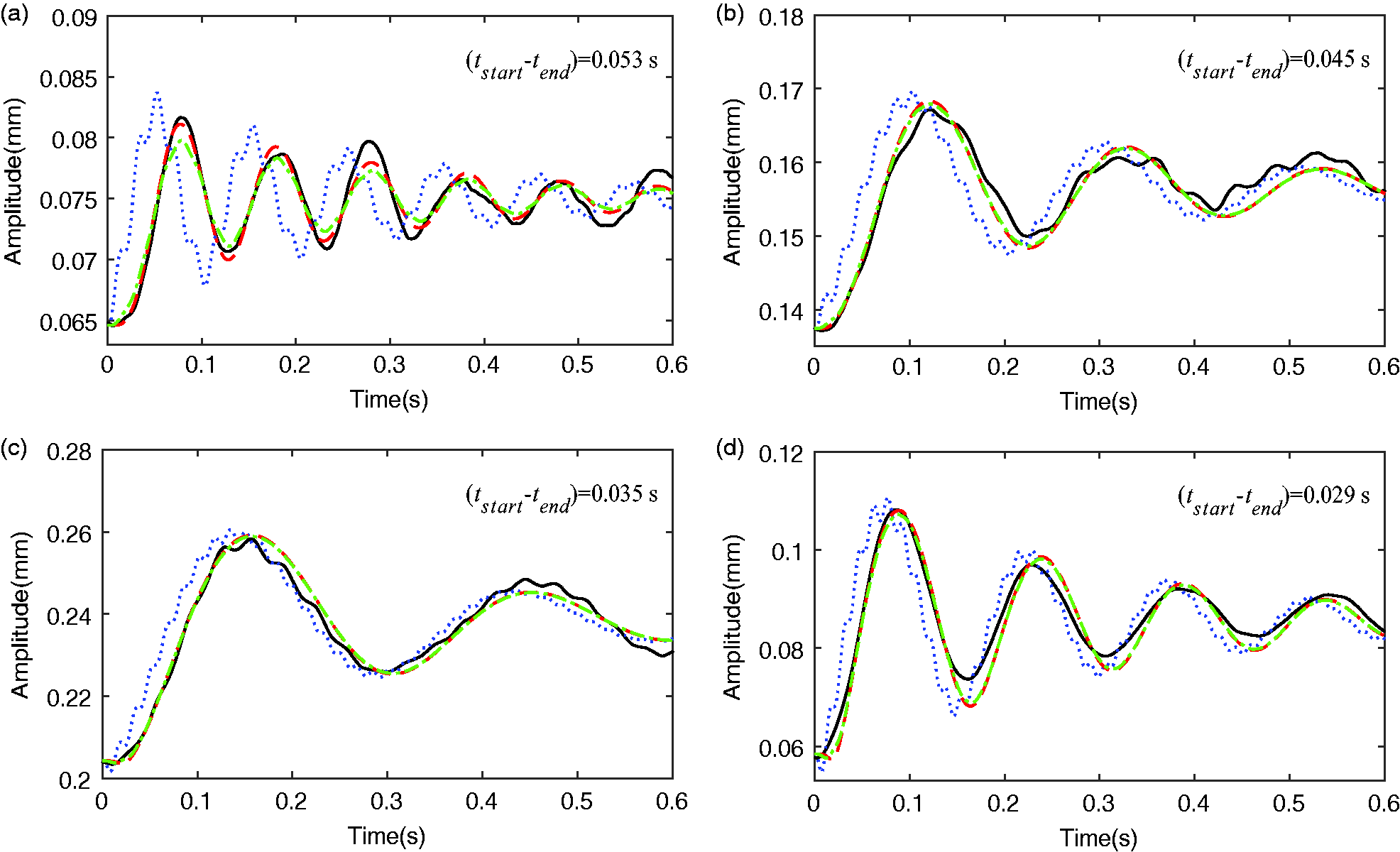
The comparison of transient response with different occurrence speeds, the measured response (solid line), the simulated response with Unit step function (dotted line), the simulated response with Cycloidal front function (dashed line) and simulated response with infinitely differentiable real function (dot-dash line). (a) 67.5°; (b) 157.5°; (c) 247.5°; (d) 337.5°.

Figure 7.

The comparison of transient response with different phase positions, the measured response (solid line), the simulated response with Unit step function (dotted line), the simulated response with Cycloidal front function (dashed line) and simulated response with Infinitely differentiable real function (dot-dash line). (a) Superposition result; (b) local amplification result.

The following conclusions can be drawn from the above comparison results:

In all cases, the simulated responses using unit step function show an obvious difference with the measured responses, especially in some significant parameters such as the peak amplitude and the fluctuation period.

The simulated responses obtained by using two continuous functions both are in good agreement with the measured responses, e.g. the subsequent fluctuation periods and the peak amplitude. It should be noted that the response obtained with the cycloidal front function are slightly larger than that with the infinitely differentiable real function, as shown in the local amplification of Figure 5(b).

The value of (t_end-t_start) varies according to different parameters. In Figure 5, it decreases from 0.040 s to 0.021 s when the magnitude increases from 6 g·mm to 24 g·mm. In Figure 6, it decreases from 0.053 s to 0.029 s when the occurrence speed increases from 1100 r/min to 2300 r/min. In Figure 7, it has no obvious change when the phase increases from 67.5° to 337.5°. As can be seen in the experiments, the magnitude and occurrence speed are the main factors affecting the total temporal duration of loading process, whereas the phase only has a weak effect. As mentioned before, the sudden unbalance mass would be released in a flying-out way when the centrifugal force overcomes the bonding force. Consequently, the greater the instantaneous centrifugal force, the shorter the duration of loading process, since the centrifugal force is mainly proportional to the magnitude and the occurrence speed of sudden unbalance, but not to the phase.

The unit step function is suitable in the case of sudden unbalance with high occurrence speed and large magnitude, because the duration of loading process is very short and even approaches zero. In the case of low occurrence speed and small magnitude, the effect of duration cannot be neglected, implying that now the continuous function should be used rather than the unit step function.

It should be noted that the above experiments and simulations are carried out in a steady-state condition. In the condition of run-up with small acceleration, the rotor motion can be approximately regarded as a steady state in a period of time. Therefore, above conclusions and values within (t_end−t_start) can still be used as a reference to the following simulations.

Transient response characteristics of sudden unbalance for a speed-varying rotor

Characteristic quantities of the transient response

For a speed-varying rotor, the response signal is amplitude modulated and frequency modulated, which has strong transient characteristics. The transient response characteristic quantities can be applied to describe the transient motion from different aspects, including the dynamic deflection, the rotation angular velocity, the precession angular velocity, the rotation angle, the precession angle and phase angle. For the rotor system, the characteristic quantities of transient response are given as follows:

Dynamic deflection r(t)

$$r\left(t\right)=\sqrt{x^2\left(t\right)+y^2\left(t\right)}$$

(10)

x(t) and y(t) are transient displacements in the x and y directions, respectively.

2. Rotation angular velocity $\dot{\phi }(t)$ and rotation angle $\phi (t)$

They have been explained in the Mathematical modeling section.

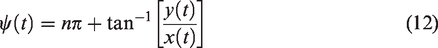
3. Precession angular velocity $\dot{\psi }(t)$

$$\dot{\psi }\left(t\right)={\left[{\tan }^{-1}\left(\frac{y\left(t\right)}{x\left(t\right)}\right)\right]}^{\prime }=\frac{\dot{y}\left(t\right)x\left(t\right)-\dot{x}\left(t\right)y\left(t\right)}{x^2\left(t\right)+y^2\left(t\right)}$$

(11)

4. Precession angle $\psi (t)$

$$\psi \left(t\right)=n\pi +{\tan }^{-1}\left[\frac{y\left(t\right)}{x\left(t\right)}\right]$$

(12)

5. Phase angle $\theta (t)$

$$\theta \left(t\right)=\phi \left(t\right)-\psi \left(t\right)$$

(13)

Simulation results and characteristic analysis

In the present study, an initial unbalance with U_i = 6 g·mm and φ_i = 135° is adopted, then some alternative values of sudden unbalance parameters are tried. For the magnitude: U_i = 5 g·mm (less than the initial unbalance) and U_i = 12 g·mm (larger than the initial unbalance). For the occurrence speed: ω_start = 2300 r/min (equal to 240.85 rad/s, above the critical speed) and ω_start = 1100 r/min (equal to 115.19 rad/s, below the critical speed). For the phase: φ_s = 0° (corresponding to the largest unbalance increase and the smallest angular change) and φ_s = 180° (corresponding to the smallest unbalance increase and the largest angular change). Newmark-β method with an integration time step of 0.0001s is used to solve the differential equations of motion. Four typical transient responses are calculated with different combinations of sudden unbalance parameters, and then the varying laws of characteristic quantities of the transient response and their correlations are analyzed.

Case 1: Sudden unbalance with U_s = 12 g·mm, ω_start = 2300 r/min and φ_s = 180°

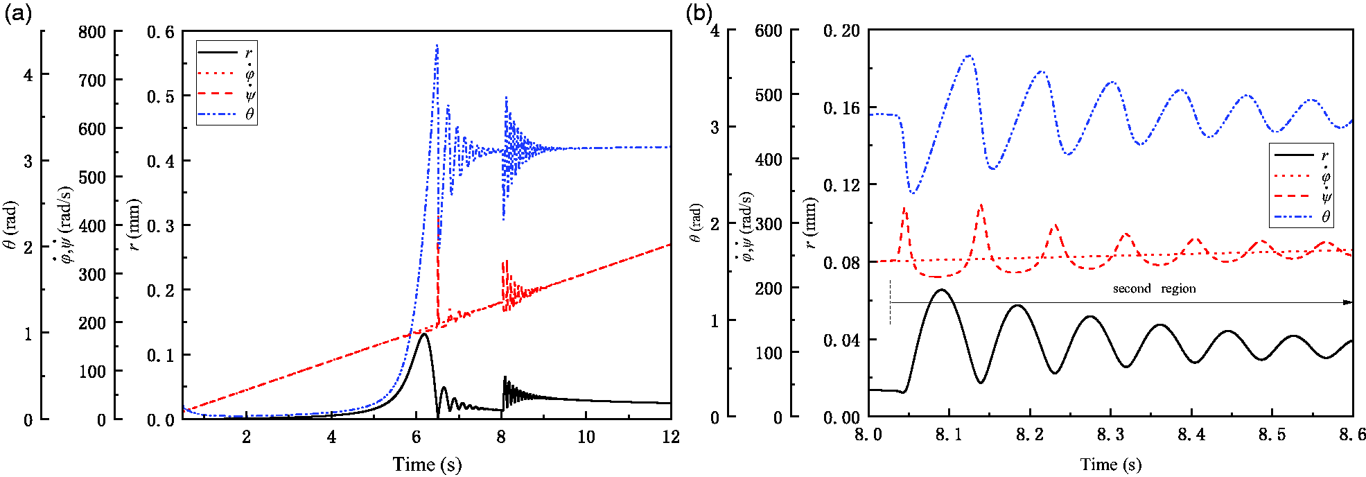
Refer to the test results in the Time-dependent function of sudden unbalance section, the value of duration is selected as (t_end-t_start) = 0.030 s. The superposition result and the local amplification result of transient responses are shown in Figure 8, and the calculation results at some key time nodes are listed in Table 3.

For convenience, the transient response of sudden unbalance can be divided into two regions in time history, according to the relationship between the precession angular velocity and rotation angular velocity, and the variation trend of phase angle, as shown in Figure 8(b). Combined with Table 3, the variations of the precession angular velocity, the phase angle and dynamic deflection in each region and corresponding relationships among them will be described in detail.

Figure 8.

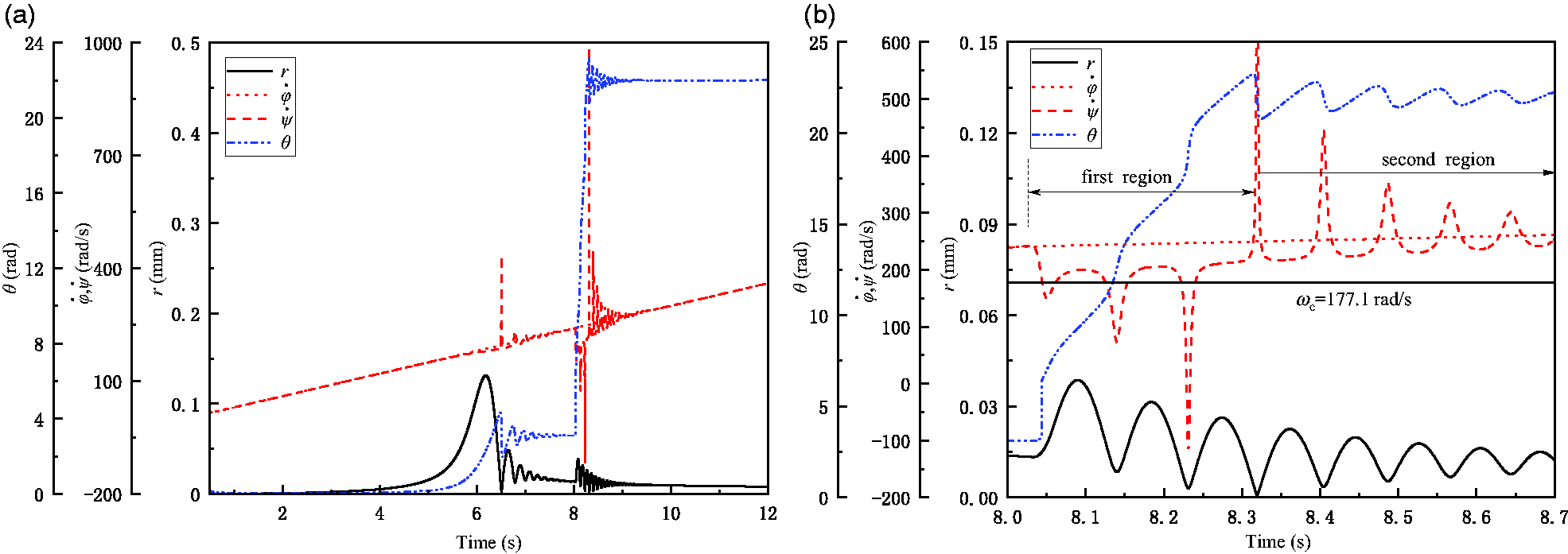
Rotor transient responses of sudden unbalance for case 1 with a = 30 rad/s², U_s = 12 g·mm, ω_start = 2300 r/min and φ_s = 180°. (a) Superposition result and (b) local amplification result.

Table 3.

Calculation results for case 1.

Region	Characteristic	$t\text{ (s)}$	$r(\text{µm})$	$\dot{\phi }(\text{rad}/\text{s)}$	$\dot{\psi }(\text{rad/s})$	$\theta (\text{rad})$
First	Occurrence	8.0285	13.36	240.85	241.57	0.981π
	$\dot{\psi }={\omega }_c$	8.0441	15.13	241.32	177.10	2.065π
	$\dot{\psi }=\min$	8.0502	17.71	241.50	149.47	2.227π
	$\dot{\psi }={\omega }_c$	8.0610	25.33	241.83	177.09	2.500π
	$r_{\max 1}$ , $\dot{\psi }\hspace{0.17em}\hspace{0.17em}\approx \hspace{0.17em}\hspace{0.17em}\max$	8.0896	38.66	242.69	199.32	2.951π
	$\dot{\psi }={\omega }_c$	8.1257	17.79	243.77	177.10	3.499π
	$r_{\min 1}$ , $\dot{\psi }=\min$	8.1397	8.43	244.19	72.86	4.002π
	$\dot{\psi }={\omega }_c$	8.1530	16.48	244.59	177.10	4.498π
	$r_{\max 2}$ , $\dot{\psi }\hspace{0.17em}\approx \hspace{0.17em}\max$	8.1837	31.44	245.51	205.01	4.959π
	$\dot{\psi }={\omega }_c$	8.2221	9.47	246.66	177.07	5.499π
	$r_{\min 2}$ , $\dot{\psi }=\min$	8.2312	3.03	246.93	−118.22	6.001π
	$\dot{\psi }={\omega }_c$	8.2401	9.11	247.20	177.07	6.499π
	$r_{\max 3}$	8.2740	26.29	248.22	211.15	6.966π
	$\dot{\psi }=\dot{\phi }$	8.3144	4.32	249.43	249.41	7.386π
Second	$r_{\min 3}$ , $\dot{\psi }=\max$	8.3193	0.75	249.58	1378.51	6.998π
	$r_{\max 4}$ , $\dot{\psi }\hspace{0.17em}\approx \hspace{0.17em}\min$	8.3610	22.57	250.83	217.38	6.971π
	$r_{\min 4}$ , $\dot{\psi }=\max$	8.4043	3.44	252.13	444.38	7.000π
	$r_{\max 5}$ , $\dot{\psi }\hspace{0.17em}\approx \hspace{0.17em}\min$	8.4450	19.82	253.35	223.65	6.975π
	$r_{\min 5}$ , $\dot{\psi }=\max$	8.4866	5.34	254.60	351.60	7.001π

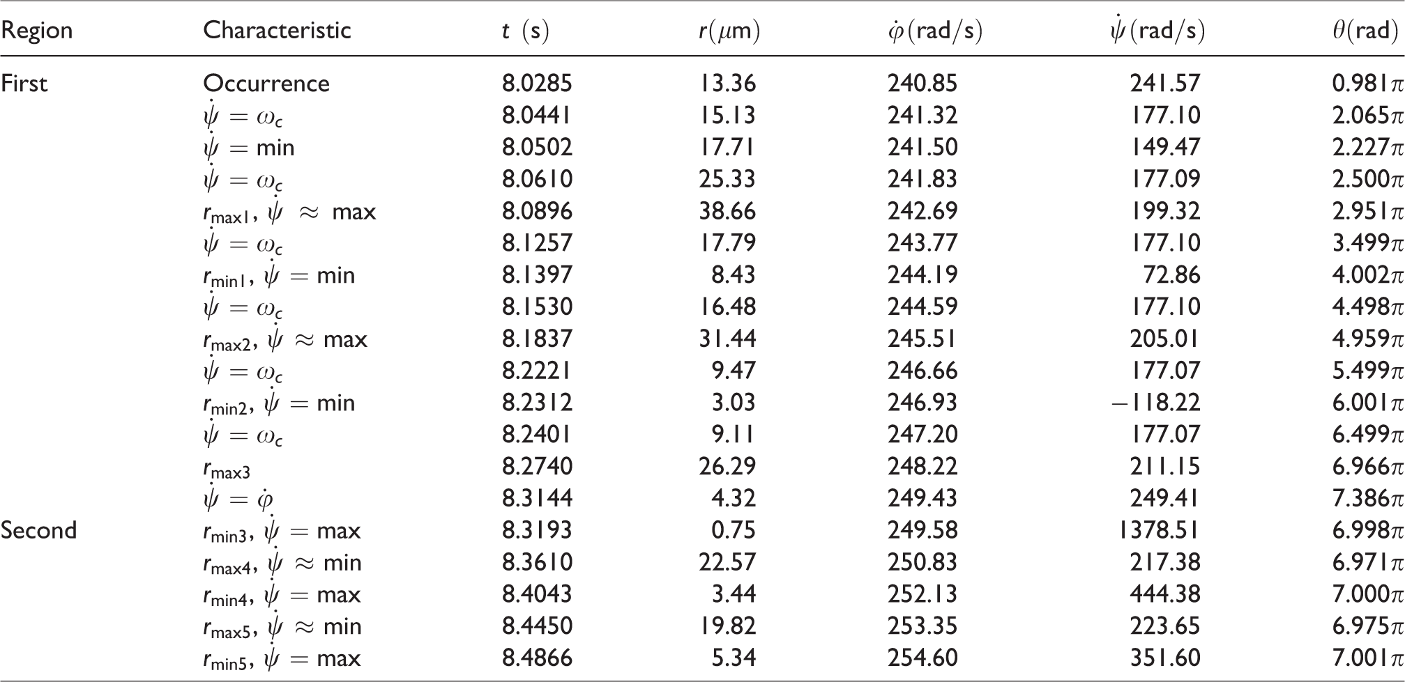
In the first region, i.e. from t  =  8.0285 s to t = 8.3144 s, the precession angular velocity is smaller than the rotation angular velocity and fluctuates around the critical speed (here the undamped critical speed is taken as ω_c = 177.1 rad/s). The fluctuation amplitude increases with time while the fluctuation period decreases with time.

The phase angle keeps jumping and increasing continually. More concretely, during the first period (incompleted) of precession angular velocity fluctuation, from t = 8.0285 s to t = 8.0610 s, the variation of phase angle at the time nodes does not follow a fixed law. It is mainly affected by the initial phase angle and the sudden unbalance phase. From t = 8.0610 s to t = 8.2401 s, the precession angular velocity fluctuation passes through two periods, and the phase angle increases by 2π rad per period. In this process, the variation of phase angle between the time nodes follows a fixed law: when the precession angular velocity is higher than the critical speed, the phase angle falls in between (2n + 1)π−0.5π rad and (2n + 1)π + 0.5π rad where n is a positive integer; when the precession angular velocity is lower than the critical speed, the phase angle falls in between 2nπ − 0.5π rad and 2nπ + 0.5π rad.

The corresponding relationships among the extreme points (maximum or minimum value) of dynamic deflection, the precession angular velocity and the phase angle are as follows: when the dynamic deflection reaches the local maximum point, the precession angular velocity will approach the local maximum point and the phase angle approximately equals to (2n + 1)π rad; when the dynamic deflection reaches the local minimum point, the precession angular velocity will reach the local minimum point with the phase angle equals to 2nπ rad.

In the second region, after t = 8.3144 s, the precession angular velocity fluctuates around the rotation angular velocity. Both the period and amplitude of fluctuation decrease with time and eventually coincide with the rotation angular velocity.

The jump finishes and the phase angle begins to fluctuate around the central value of θ = 7π rad. Similarly, both the period and amplitude of fluctuation decrease with the time and eventually tend to θ = 7π rad. Compared with the initial value of phase angle before sudden unbalance occurs, it has increased by a total of (2 × 3π) rad, which indicates the phase angle will increase by 2nπ rad at the end of the transient process, where n is the number of troughs below the critical speed of precession angular velocity fluctuation in the first region.

The corresponding relationships among the extreme points of dynamic deflection, the precession angular velocity and the phase angle are as follows: when the dynamic deflection reaches the local maximum point, the precession angular velocity will approach the local minimum point with the phase angle approximately equals to (2 × 3 + 1)π rad; when the dynamic deflection reaches the local minimum point, the precession angular velocity will reach the local maximum point with the phase angle equal to (2 × 3 + 1)π rad.

It illustrates that the corresponding relationships among the local minimum point of dynamic deflection, the precession angular velocity and the phase angle are more accurate than those of the local maximum point.

Case2: Sudden unbalance with U_s = 12 g·mm, ω_start = 2300 r/min, φ_s = 0° and (t_end-t_start) = 0.030 s

The superposition result and the local amplification result of transient responses are shown in Figure 9, and the calculation results at some key time nodes are listed in Table 4.

Table 4.

Calculation results for case 2.

Region	Characteristic	$t\left(\text{s}\right)$	$r\left(\mu \text{m}\right)$	$\dot{\phi }\left(\text{rad}/\text{s}\right)$	$\dot{\psi }\left(\text{rad}/\text{s}\right)$	$\theta \left(\text{rad}\right)$
Second	Occurrence	8.0285	13.36	240.85	241.57	0.981π
	$r_{\max 1}$	8.0904	65.49	242.71	216.84	0.971π
	$r_{\min 1}$ , $\dot{\psi }=\max$	8.1389	17.49	244.17	327.84	0.999π
	$r_{\max 2}$ , $\dot{\psi }\hspace{0.17em}\approx \hspace{0.17em}\max$	8.1842	57.53	245.53	223.17	0.975π
	$r_{\min 2}$ , $\dot{\psi }=\min$	8.2306	22.34	246.92	297.10	0.998π
	$r_{\max 3}$ , $\dot{\psi }\hspace{0.17em}\approx \hspace{0.17em}\max$	8.2744	51.74	248.23	229.18	0.978π
	$r_{\min 3}$ , $\dot{\psi }=\min$	8.3189	25.62	249.57	283.27	0.998π
	$r_{\max 4}$ , $\dot{\psi }\hspace{0.17em}\approx \hspace{0.17em}\max$	8.3612	47.45	250.83	234.73	0.980π
	$r_{\min 4}$ , $\dot{\psi }=\min$	8.4041	27.85	252.12	276.15	0.999π

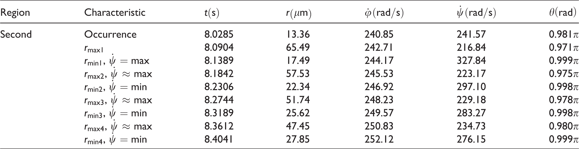
As shown in Figure 9, the precession angular velocity directly enters into the second region. Correspondingly, the phase angle fluctuates around the central value of θ = π rad without the leap increase.

Figure 9.

Rotor transient responses of sudden unbalance for case 2 with a = 30 rad/s², U_s = 12 g·mm, ω_start = 2300 r/min and φ_s = 0°. (a) Superposition result; (b) local amplification result.

In the second region, the corresponding relationships among the extreme points of dynamic deflection, the precession angular velocity and the phase angle are consistent with those in Case 1. Similarly, the corresponding relationships among the local minimum point of dynamic deflection, the precession angular velocity and the phase angle are more accurate than those of the local maximum point.

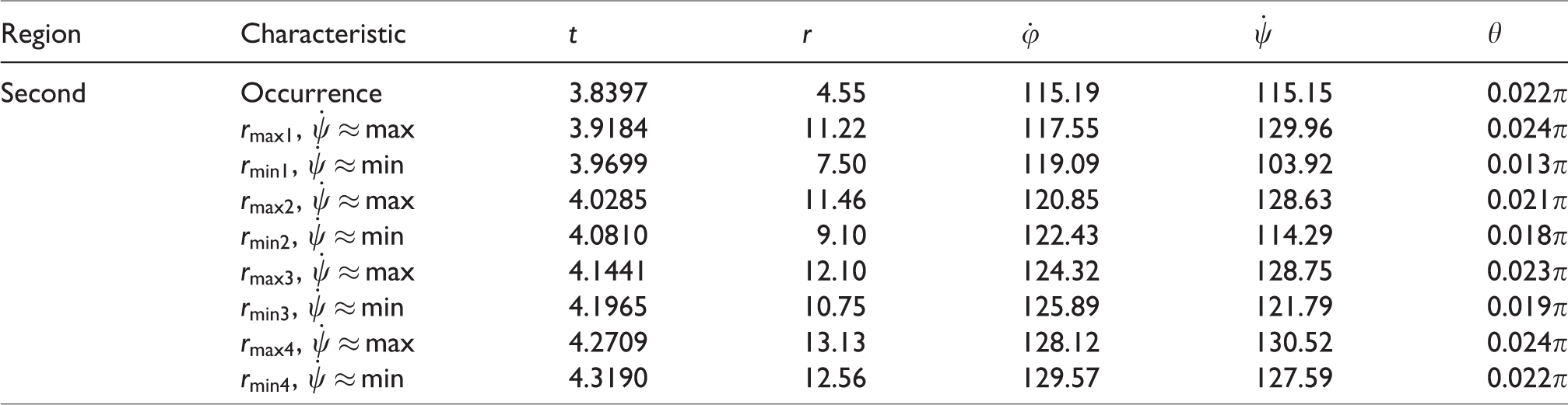
Case3: Sudden unbalance with U_s = 5 g·mm, ω_start = 1100 r/min, φ_s = 180° and (t_end-t_start) = 0.059 s

The superposition result and the local amplification result of transient responses are shown in Figure 10, and the calculation results at some key time nodes are listed in Table 5.

Table 5.

Calculation results for case 3.

Region	Characteristic	$t\left(\text{s}\right)$	$r\left(\mu \text{m}\right)$	$\dot{\phi }(\text{rad/s})$	$\dot{\psi }(\text{rad/s})$	$\theta (\text{rad})$
First	Occurrence	3.8397	4.55	115.19	115.15	0.022π
	$\dot{\psi }={\omega }_c$	3.8989	2.24	116.96	177.14	−0.493π
	$r_{\min 1}$ , $\dot{\psi }\hspace{0.17em}\approx \hspace{0.17em}\max$	3.9201	1.44	117.60	214.25	−1.021π
	$\dot{\psi }={\omega }_c$	3.9398	2.01	118.19	177.21	−1.505π
	$r_{\max 1}$ , $\dot{\psi }\hspace{0.17em}\approx \hspace{0.17em}\min$	3.9672	2.76	119.01	159.30	−1.912π
	$\dot{\psi }={\omega }_c$	4.0092	1.41	120.27	177.11	−2.476π
	$r_{\min 2}$ , $\dot{\psi }=\max$	4.0276	0.67	120.82	257.36	−2.999π
	$\dot{\psi }={\omega }_c$	4.0451	1.26	121.35	177.03	−3.508π
	$r_{\max 2}$ , $\dot{\psi }\hspace{0.17em}\approx \hspace{0.17em}\min$	4.0833	2.25	122.49	154.26	−3.971π
	$\dot{\psi }={\omega }_c$	4.1347	0.42	124.04	177.30	−4.485π
	$r_{\min 3}$ , $\dot{\psi }=\max$	4.1424	0.07	124.27	847.41	−5.001π
	$\dot{\psi }={\omega }_c$	4.1493	0.37	124.47	177.45	−5.506π
	$r_{\max 3}$	4.1998	1.93	125.99	149.69	−5.950π
	$\dot{\psi }=\dot{\phi }$	4.2471	0.87	127.41	127.47	−6.210π
Second	$r_{\min 4}$ , $\dot{\psi }\hspace{0.17em}\approx \hspace{0.17em}\min$	4.2647	0.41	127.94	46.57	−5.989π
	$r_{\max 4}$ , $\dot{\psi }\hspace{0.17em}\approx \hspace{0.17em}\max$	4.3310	1.76	129.93	145.22	−5.972π
	$r_{\min 5}$ , $\dot{\psi }\hspace{0.17em}\approx \hspace{0.17em}\min$	4.3963	0.83	131.88	106.18	−5.987π
	$r_{\max 5}$ , $\dot{\psi }\hspace{0.17em}\approx \hspace{0.17em}\max$	4.4709	1.73	134.12	143.14	−5.969π
	$r_{\min 6}$ , $\dot{\psi }\hspace{0.17em}\approx \hspace{0.17em}\min$	4.5406	1.21	136.21	126.25	−5.976π
	$r_{\max 6}$ , $\dot{\psi }\hspace{0.17em}\approx \hspace{0.17em}\max$	4.6268	1.84	138.80	143.12	−5.965π

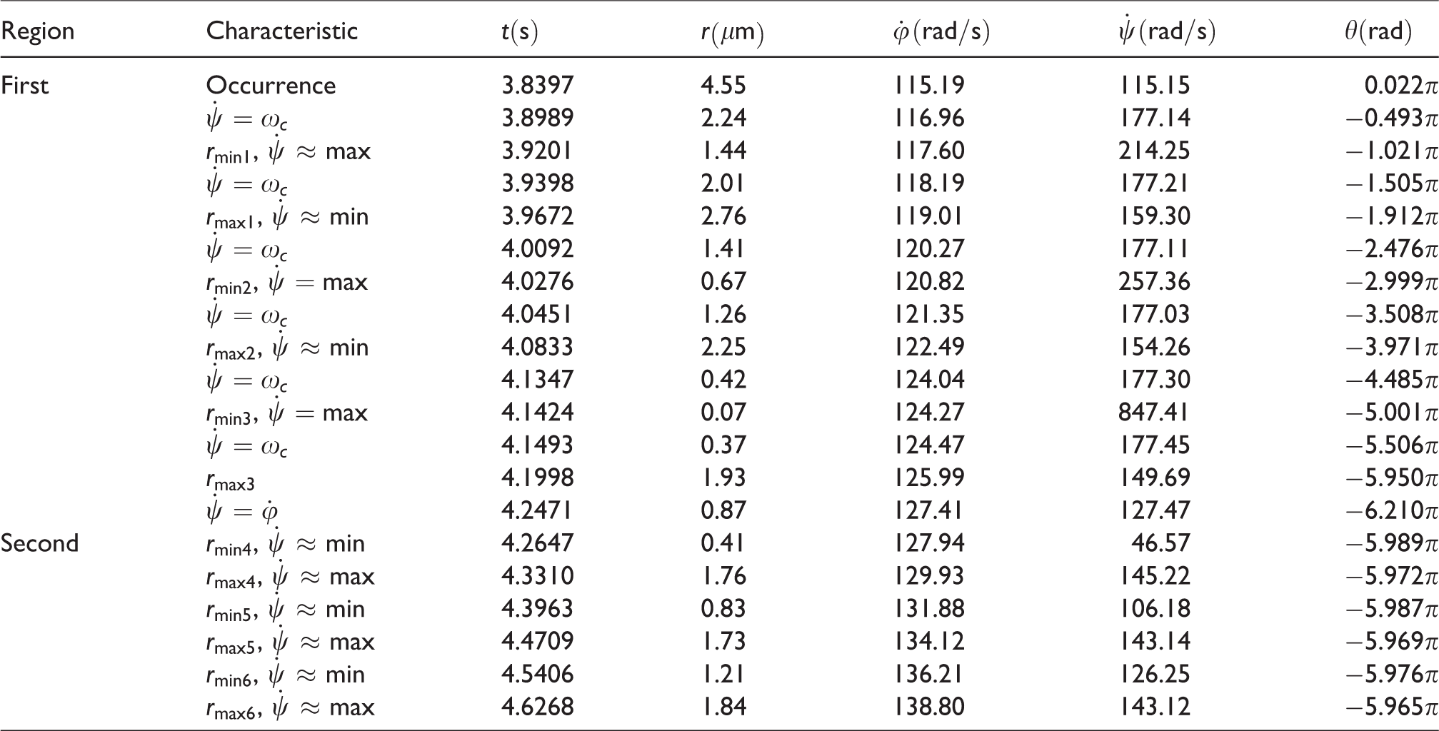
Same as in Case 1, two regions are divided as shown in Figure 10(b). The first region is between t = 3.8397 s and t = 4.2471 s, in which the precession angular velocity is always higher than the rotation angular velocity and fluctuates around the critical speed. Corresponding to the variation of precession angular velocity, the phase angle keeps diving and decreasing continually. During the first period (incompleted) of precession angular velocity fluctuation, between t = 3.8397 s and t = 3.9398 s, the variation of phase angle at the time nodes does not follow a fixed law. From t = 3.9398 s to t = 4.1493 s, the precession angular velocity fluctuation passes through two periods and the phase angle decreases by 2π rad per period. In this process, the phase angle variation between the time nodes approximately follows the following law: when the precession angular velocity is lower than the critical speed, the phase angle falls in between −2nπ + 0.5π rad and −2nπ−0.5π rad where the n is a positive integer; when the precession angular velocity is higher than the critical speed, the phase angle falls in between − (2n + 1)π + 0.5π rad and −(2n + 1)π−0.5π rad.

Figure 10.

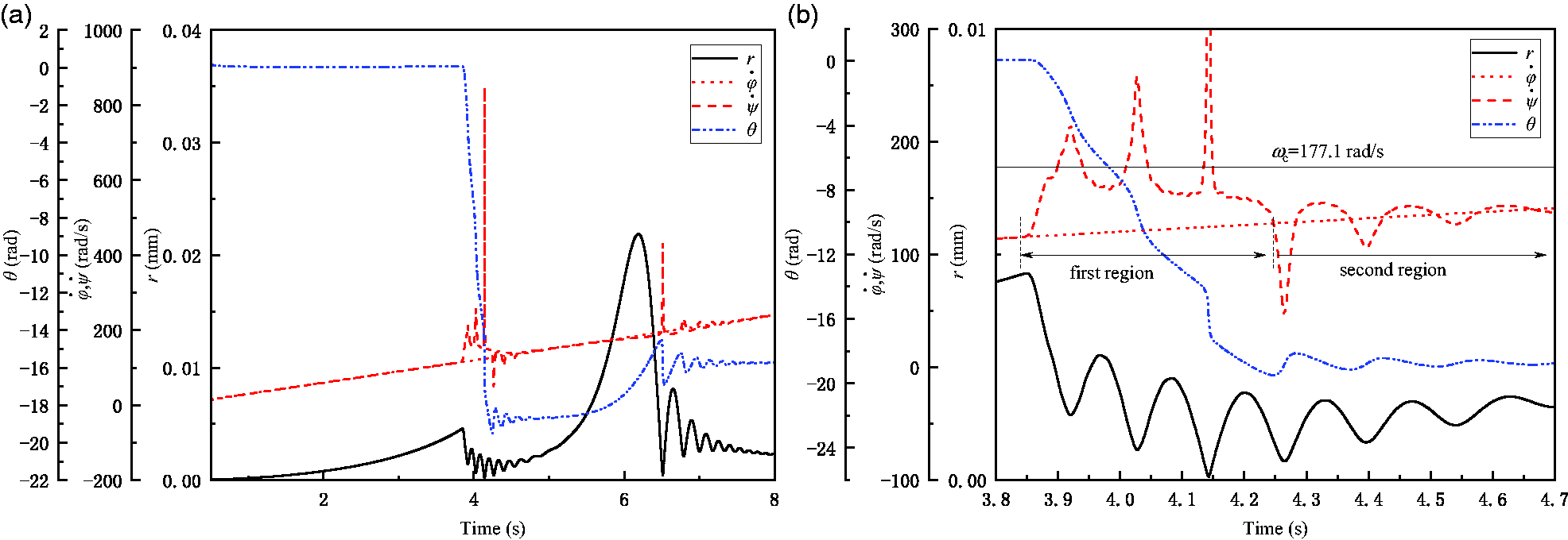
Rotor transient responses of sudden unbalance for case 3 with a = 30 rad/s², U_s = 5 g·mm, ω_start = 1100 r/min and φ_s = 180°. (a) Superposition result; (b) local amplification result.

The corresponding relationships among the extreme points of dynamic deflection, the precession angular velocity and phase angle can be summarized as follows: when the dynamic deflection reaches the local maximum point, the precession angular velocity will approach the local minimum point with the phase angle approximately equals to -2nπ rad; when the dynamic deflection reaches the local minimum point, the precession angular velocity will reach the local maximum point with the phase angle equals to −(2n + 1)π rad.

In the second region, after t = 4.2471 s, the precession angular velocity fluctuates around the rotation angular velocity, while the phase angle fluctuates around a central value of θ=−6π rad. Compared with the initial value of phase angle before the sudden unbalance occurs, it has decreased by a total of (2 × 3π) rad, implying the phase angle would decrease by 2nπ rad at the end of the transient process, where n is the number of troughs above the critical speed of precession angular velocity fluctuation in the first region.

The corresponding relationships among the extreme points of dynamic deflection, the precession angular velocity and the phase angle are as follows: when the dynamic deflection reaches its local maximum point, the precession angular velocity will approach the local maximum point with the phase angle approximately equal to −(2 × 3)π rad; when the dynamic deflection reaches its local minimum point, the precession angular velocity will approach the local minimum point with the phase angle approximately equal to −(2 × 3)π rad.

The above results indicate that the corresponding relationships among the extreme points of dynamic deflection, the precession angular velocity and phase angle are approximate, not accurate as those in Case 1.

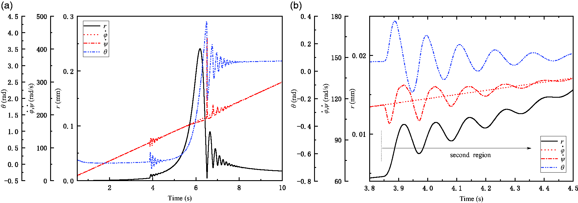
Case4: Sudden unbalance with U_s = 5 g·mm, ω_start = 1100 r/min, φ_s = 0° and (t_end-t_start) = 0.059 s

The superposition result and the local amplification result of the transient responses are shown in Figure 11, and the calculation results at some critical time nodes are listed in Table 6.

From Figure 11 and Table 6, it can be seen that the variation characteristics of transient response are similar to those in Case 2. The difference is that the phase angle fluctuates around zero line before critical speed, so the phase angle corresponding to the maximum and minimum points of the transient dynamic deflection fluctuation is close to zero.

Figure 11.

Rotor transient responses of sudden unbalance for case 4 with a = 30 rad/s², U_s = 5 g·mm, ω_start = 1100 r/min and φ_s = 0°. (a) 1 g·mm; (b) 4 g·mm; (c) 5 g·mm; (d) 7 g·mm; (e) 10 g·mm; (f) 12 g·mm.

Table 6.

Calculation results for case 4.

Region	Characteristic	$t$	$r$	$\dot{\phi }$	$\dot{\psi }$	$\theta$
Second	Occurrence	3.8397	4.55	115.19	115.15	0.022π
	$r_{\max 1}$ , $\dot{\psi }\approx \max$	3.9184	11.22	117.55	129.96	0.024π
	$r_{\min 1}$ , $\dot{\psi }\approx \min$	3.9699	7.50	119.09	103.92	0.013π
	$r_{\max 2}$ , $\dot{\psi }\approx \max$	4.0285	11.46	120.85	128.63	0.021π
	$r_{\min 2}$ , $\dot{\psi }\approx \min$	4.0810	9.10	122.43	114.29	0.018π
	$r_{\max 3}$ , $\dot{\psi }\approx \max$	4.1441	12.10	124.32	128.75	0.023π
	$r_{\min 3}$ , $\dot{\psi }\approx \min$	4.1965	10.75	125.89	121.79	0.019π
	$r_{\max 4}$ , $\dot{\psi }\approx \max$	4.2709	13.13	128.12	130.52	0.024π
	$r_{\min 4}$ , $\dot{\psi }\approx \min$	4.3190	12.56	129.57	127.59	0.022π

Sudden unbalance parameter region

From the previous analysis, it can be seen that the transient response characteristics of rotor system has an obvious change for different sudden unbalance parameters. Three variation forms of transient response characteristics can be summarized as below:

The transient process has a type of first region where the precession angular velocity fluctuates around the critical speed and always be less than the rotation angular velocity, while the phase angle has a leap increase by 2nπ rad. Detailed varying laws in the first and second regions can be seen in Case 1.

The transient process has a type of first region where the precession angular fluctuates around the critical speed and always be higher than the rotation angular velocity, while the phase angle has a leap decrease by 2nπ rad. Detailed varying laws in the first and second region can be seen in Case 3.

The transient process has the unique second region where the precession angular fluctuates around the rotation angular velocity, while the phase angle fluctuates around a central value. The central value is 0 rad when the occurrence speed is subcritical and 2(n+1)π rad when the occurrence speed is supercritical. Detailed varying laws can be seen in Cases 2 and 4.

In this section, the correspondences between the transient response characteristics of rotor system and the sudden unbalance parameters are studied. The sudden unbalance parameter regions corresponding to different variation forms are calculated as shown in Figure 12. Six levels of sudden unbalance are chosen: 1 g·mm, 4 g·mm, 5 g·mm, 7 g·mm, 10 g·mm and 12 g·mm. The abscissa represents the phase of sudden unbalance, and the ordinate represents the occurrence speed (expressed by the speed ratio ω_start/ω_c here). The phase and the occurrence speed studied are in the range of φ_s  ∈  [0°, 180°] and ω_start/ω_c ∈ [0.2, 2.0], respectively.

Figure 12.

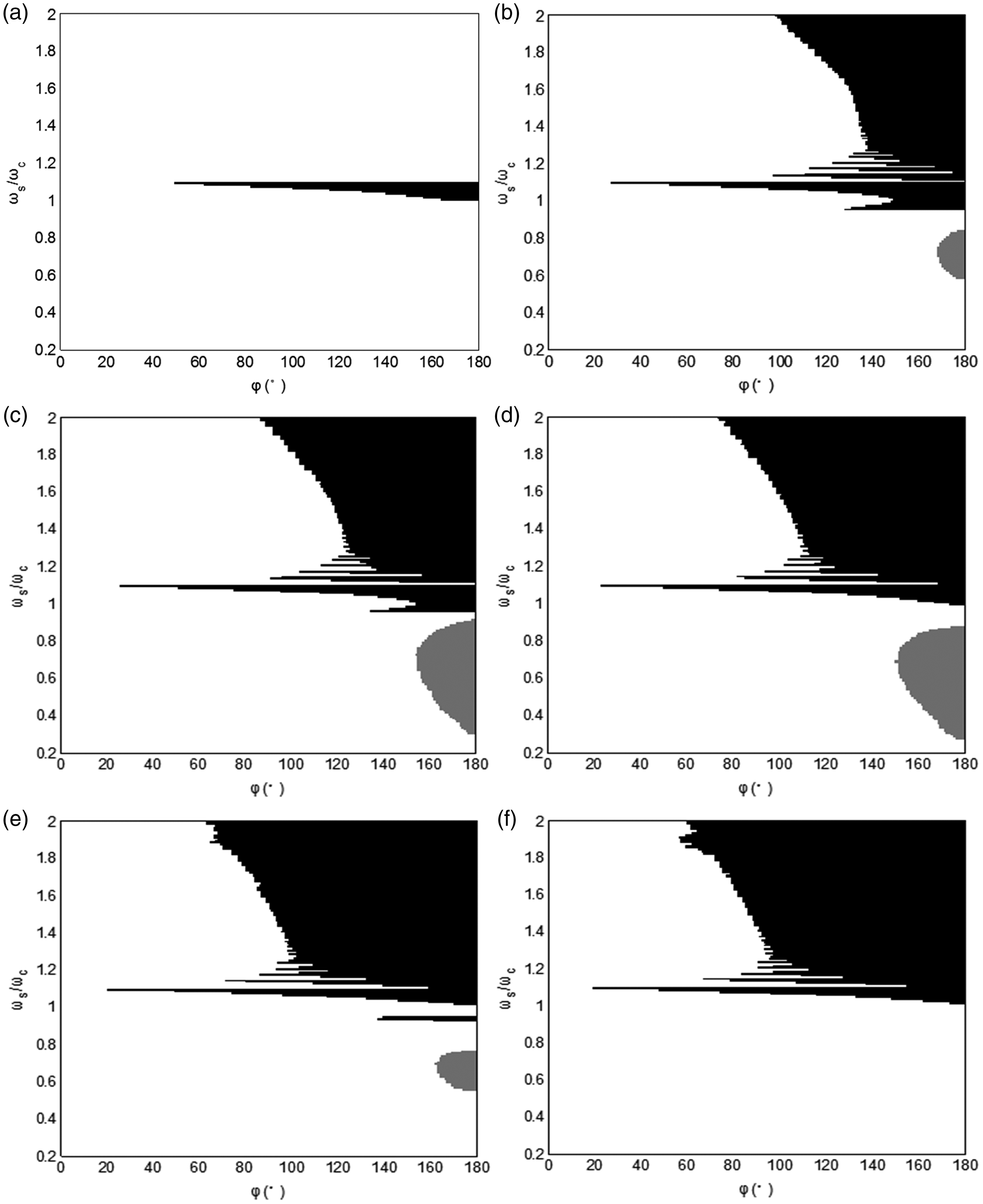
Sudden unbalance parameter region, variation form I (black area), variation form II (gray area) and variation form III (white area).(a) 1 g·mm, (b) 4 g·mm, (c) 5 g·mm, (d) 7 g·mm, (e) 10 g·mm and (f) 12 g·mm.

From Figure 12, the distribution range of the phase and occurrence speed corresponding to different variation forms is shown intuitively for different cases of sudden unbalance magnitude. It should be noted that the variation form I can occur in the critical area or over the critical speed, while the variation form II will only appear before the critical speed. When the magnitude of sudden unbalance is much less or much larger than the initial unbalance (e.g. 1 g·mm, 12 g·mm), the parameter region corresponding to variation form 2 will disappear.

Identification of initial unbalance based on the transient response data of sudden unbalance

From the above analysis, it can be found that a certain correspondence exists between the minimum point of dynamic deflection fluctuation and the phase angle during the transient process of sudden unbalance. Based on the above conclusion, the momentary positions of geometric and mass center of the disc at different time instants are illustrated via introducing the key-phase signal. The angular variations between different momentary positions are analyzed so as to identify the phase and magnitude of unbalance.

Identification of synthetic unbalance angle δ

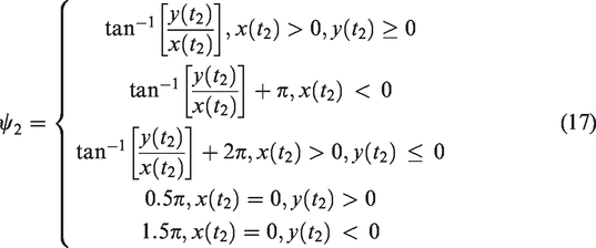
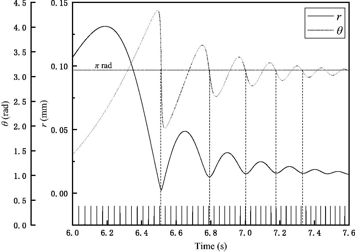
The transient response data of sudden unbalance contains the information of synthetic unbalance which is composed of initial unbalance and sudden unbalance. Take Case 1 in Sudden unbalance parameter region section for example, Figure 13 shows the relationship between the transient dynamic deflection and the key-phase signal. As shown in Table 3, the corresponding phase angle of the first two minimum points of dynamic deflection fluctuation is 2nπ rad. Denote the corresponding moment of the minimum point by t₂. The solid line in Figure 14(a) represents the momentary position of disc at instant t₂. The three points including the origin of coordinates O, the center of mass C₂ and the geometric center O₂ are collinear, and C₂ is located at the outer end of the connecting line between O and O₂. t₁ represents the corresponding instant of adjacent key-phase signal before the minimum point, and the momentary position of disc at t₁ is denoted by the dashed line in Figure 14(a). In a similar way, the corresponding phase angle of the third and following minimum points of dynamic deflection response fluctuation is (2 × 3 + 1)π rad. Denote the corresponding moment of the minimum point by ${t^{\prime }}_2$ . The solid line in Figure 14(b) represents the momentary position of disc at ${t^{\prime }}_2$ . The three points including the origin of coordinates O, the center of mass C₂ and the geometric center O₂ are collinear; C₂ is located in the middle of the connecting line between O and O₂. ${t^{\prime }}_1$ represents the corresponding instant of adjacent key-phase signal before the minimum point, and the momentary position at ${t^{\prime }}_1$ is denoted by the dashed line in Figure 14(b).

Figure 13.

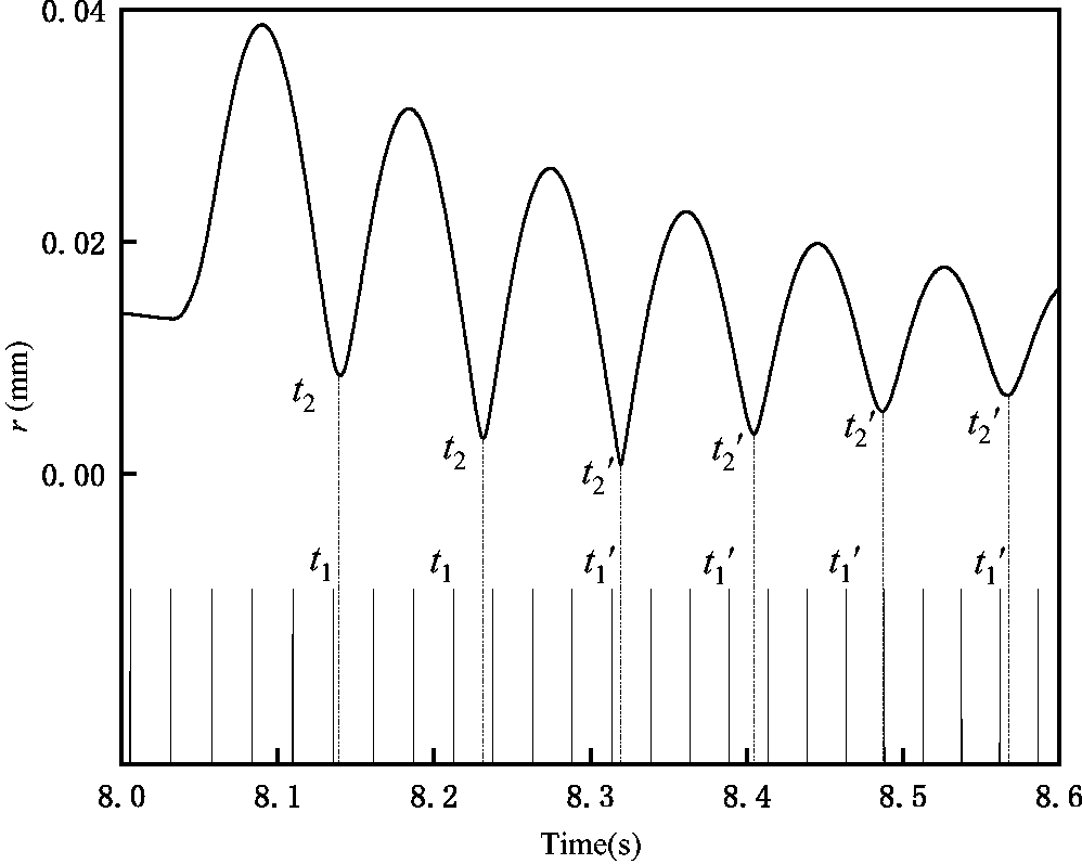
The relationship between transient dynamic deflection and key-phase signal. (a) t₁ and t₂ moment and (b) ${t^{\prime }}_1$ and ${t^{\prime }}_2$ moment.

Figure 14.

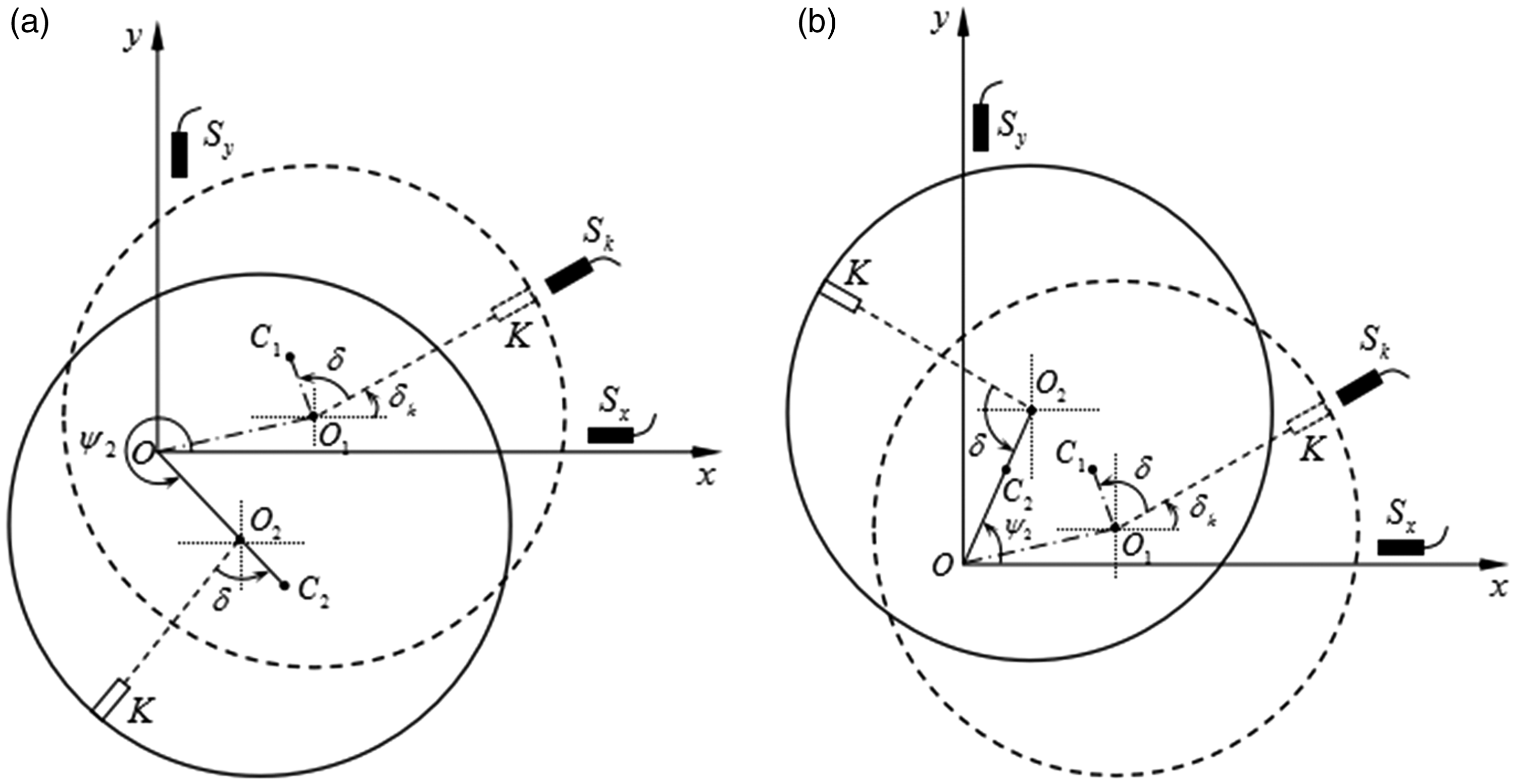
Schematic diagram of momentary position of the disc at different moments. (a) t₁ and t₂ moment; (b) ${t^{\prime }}_1$ and ${t^{\prime }}_2$ moment.

As shown in Figure 15(a), the angular relationship of momentary position of the disc at t₁ and t₂ can be obtained through a translation, and the relationship of ${t^{\prime }}_1$ and ${t^{\prime }}_2$ is drawn in Figure 15(b). In Figure 14 and 15, K, S_k and δ_k represent the key slot, the key-phase signal sensor and the intersection angle (the horizontal installation angle is 0°) between the key-phase signal sensor and x axis; S_x and S_y are the displacement sensors of x and y directions; ψ₂ represents precession angle of the rotor at t₂ or ${t^{\prime }}_2$ . δ is the synthetic unbalance angle which represents the angular position of synthetic unbalance to the key-slot.

Figure 15.

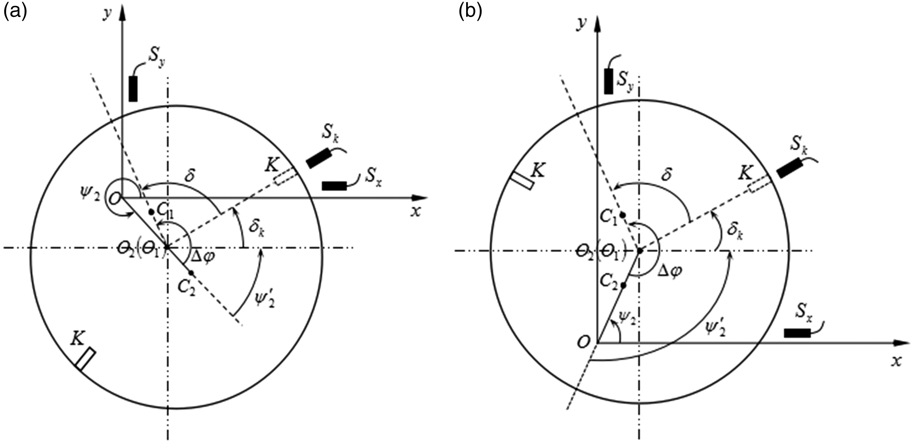
Schematic diagram of angular relationships of momentary position at different moments.

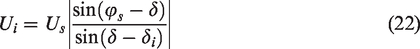
As shown in Figure 15(a), at t₁ and t₂, the δ can be expressed as

$$\delta =2\pi -\left({\phi }_2-{\phi }_1\right)-{{\psi }^{\prime }}_2-{\delta }_k$$

(14)

$${{\psi }^{\prime }}_2=2\pi -{\psi }_2$$

(15)

Hence

$$\delta ={\psi }_2-\left({\phi }_2-{\phi }_1\right)-{\delta }_k$$

(16)

where ψ₂ can be obtained by

$${\psi }_2=\{\begin{array}{c}{\tan }^{-1}\left[\frac{y(t_2)}{x(t_2)}\right],x(t_2)>0,y(t_2)\ge 0\\ {\tan }^{-1}\left[\frac{y(t_2)}{x(t_2)}\right]+\pi ,x(t_2)<0\\ {\tan }^{-1}\left[\frac{y(t_2)}{x(t_2)}\right]+2\pi ,x(t_2)>0,y(t_2)\le 0\\ 0.5\pi ,x(t_2)=0,y(t_2)>0\\ 1.5\pi ,x(t_2)=0,y(t_2)<0\end{array}$$

(17)

(φ₂−φ₁) represents the rotation angle from t₁ to t₂ moment, here we consider that angular acceleration a is constant, thus

$${\phi }_2-{\phi }_1=\frac{1}{2}a\left(t_2^2-t_1^2\right)$$

(18)

As shown in Figure 15(b), at ${t^{\prime }}_1$ and ${t^{\prime }}_2$ , δ would be expressed as

$$\delta =2\pi -\left({\phi }_2-{\phi }_1\right)-{{\psi }^{\prime }}_2-{\delta }_k$$

(19)

while

$${{\psi }^{\prime }}_2=\pi -{\psi }_2$$

(20)

Hence

$$\delta =\pi +{\psi }_2-\left({\phi }_2-{\phi }_1\right)-{\delta }_k$$

(21)

Identification of initial unbalance angle δ_i

Figure 16 shows the relationship among the dynamic deflection, the phase angle and the key-phase signal when the rotor runs across the critical speed region. The transient response data only contains the initial unbalance information since the sudden unbalance does not occur. The corresponding phase angle of minimum points of transient dynamic deflection fluctuation is π rad in the critical speed region. Therefore, the momentary positions and angular relationships of the disc in the corresponding moments of minimum point and adjacent key-phase signal pulse before minimum point are the same as shown in Figures 14(b) and 15(b). Thus, the initial unbalance angle δ_i can be identified by equation (21).

Figure 16.

The relationship among transient dynamic deflection, phase angle and key-phase signal in critical speed region.

Identification of initial unbalance magnitude U_i

Since magnitude U_s and phase φ_s of sudden unbalance are known, and initial unbalance angel δ_i and synthetic unbalance angle δ both have been identified, the magnitude of initial unbalance can be obtained by the vector composition relation as follows

$$U_i=U_s\left|\frac{\sin ({\phi }_s-\delta )}{\sin (\delta -{\delta }_i)}\right|$$

(22)

As a result, the angle(phase) and magnitude of the initial unbalance could be identified by utilizing the transient response data in the critical region and the sudden unbalance response data. All information is collected in just one single run-up.

Identification results and discussions

In this section, the identification procedure is performed by numerical simulations. The proposed identification method is examined by comparing the identified value with the set value. The initial unbalance is set as U_i = 6 g·mm and φ_i = 135°. The transient response calculated from the FE model is adopted as the measured response. The first six minimum points of dynamic deflection in the sudden unbalance process are selected to identify the synthetic unbalance angle. Similarly, we take the first six minimum points of dynamic deflection in the critical resonance region to identify the initial unbalance angle. The influences due to different parameters of sudden unbalance on the identification error are analyzed, including the magnitude, the occurrence speed and the phase.

The effect of magnitude is investigated while fixing the occurrence speed and phase: ω_start = 2400 r/min and φ_s = 135°. Here, the magnitude is described by the ratio U_s/U_i, which increases from 0.05 to 5.0. The results of identification are shown in Table 7.

Table 7.

Identification results with different U_s/U_i.

Us/Ui	Unbalance magnitude (g·mm)	Magnitude error (%)	Phase (degree)	Phase error (%)
0.05	5.35	−10.83
0.5	6.10	1.66
1.0	6.07	1.16	135.85	0.63
3.0	6.11	1.83
5.0	6.04	0.67

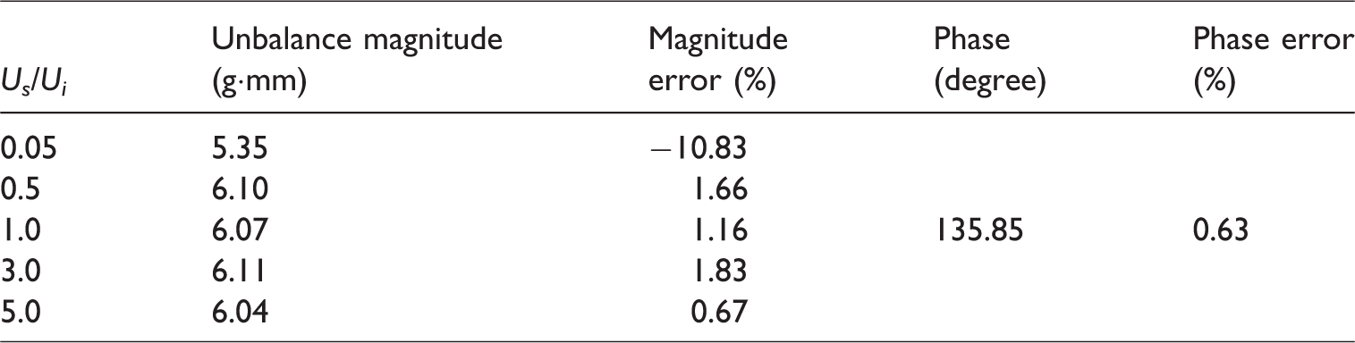
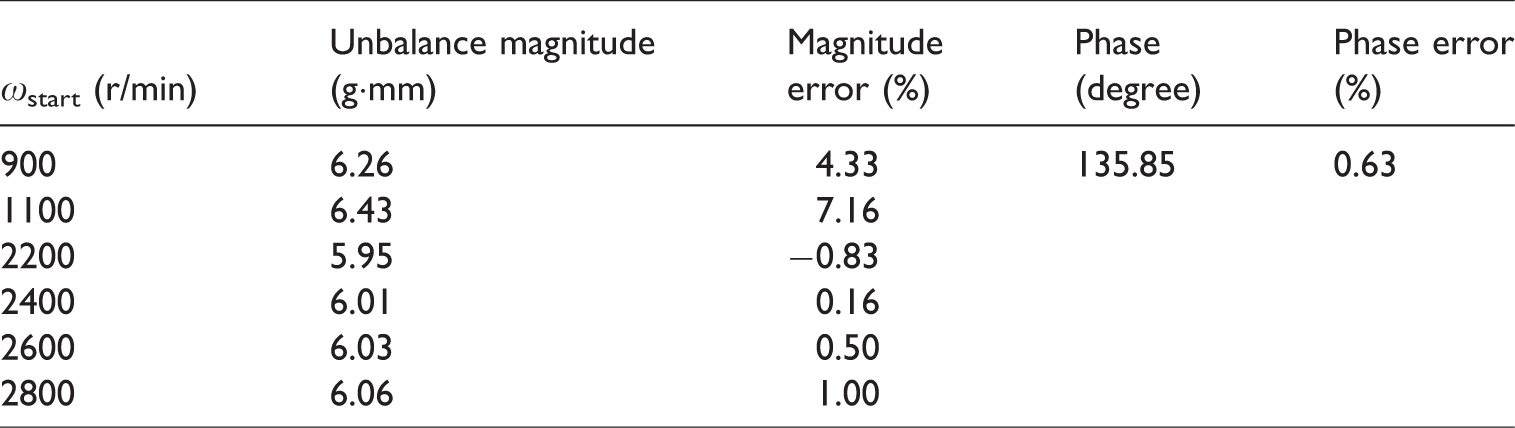
Table 8 shows the identification results for different occurrence speeds. The identification procedure is performed using two occurrence speeds below the critical speed (900 and 1100 r/min), and four speeds above the critical speed (2200, 2400, 2600 and 2800 r/min). The magnitude and the phase are kept fixed: U_s = 12 g·mm and φ_s = 135°.

Table 8

Identification results with different ω_start.

ωstart (r/min)	Unbalance magnitude (g·mm)	Magnitude error (%)	Phase (degree)	Phase error (%)
900	6.26	4.33	135.85	0.63
1100	6.43	7.16
2200	5.95	−0.83
2400	6.01	0.16
2600	6.03	0.50
2800	6.06	1.00

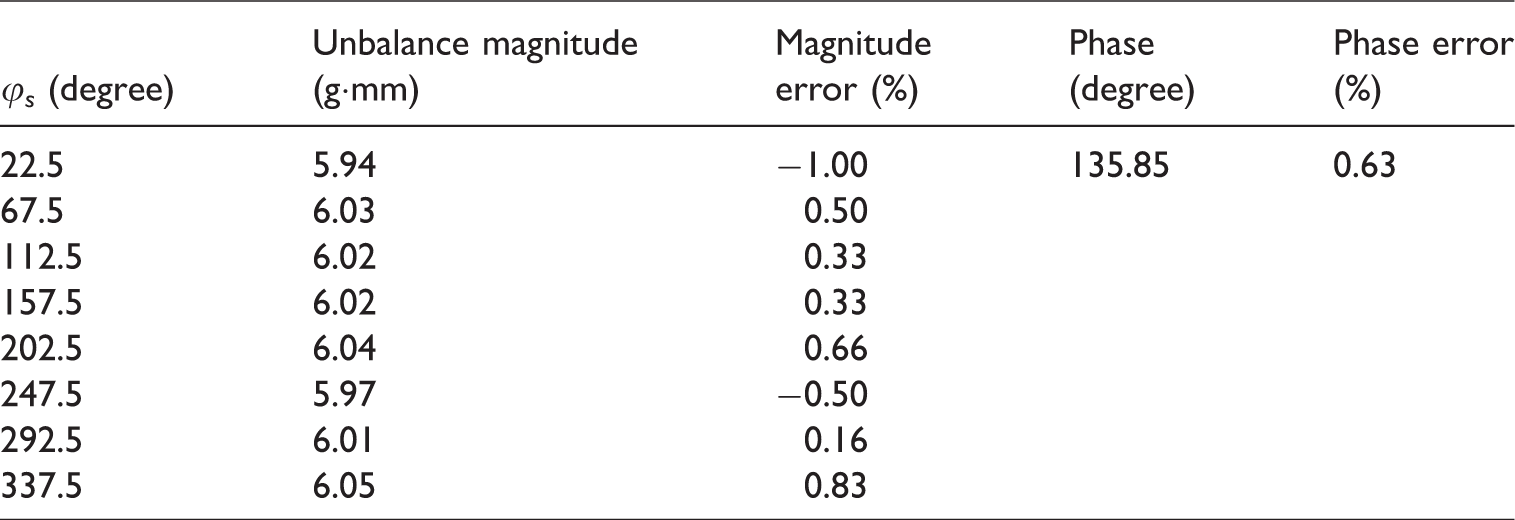
The identification results are presented with the phase varying from 22.5° to 337.5° with 45° spacing, as shown in Table 9. The magnitude and the occurrence speed are kept constant which are 12 g·mm and 2400 r/min, respectively.

Table 9.

Identification results with different φ_s.

φs (degree)	Unbalance magnitude (g·mm)	Magnitude error (%)	Phase (degree)	Phase error (%)
22.5	5.94	−1.00	135.85	0.63
67.5	6.03	0.50
112.5	6.02	0.33
157.5	6.02	0.33
202.5	6.04	0.66
247.5	5.97	−0.50
292.5	6.01	0.16
337.5	6.05	0.83

From the above numerical simulations, we can draw the conclusions as follows:

As can be seen in Tables 7 to 9, the identification of initial unbalance phase keeps the same value and shows a good accuracy. It is noted that the change of sudden unbalance only affects the identification of initial unbalance magnitude.

According to Table 7, it can be observed the results of the identification are all satisfactory when the ratio U_s/U_i varies from 0.5 to 5.0. When the ratio is U_s/U_i = 0.05, the identification shows a poor result. This is due to the reason that the transient fluctuation of dynamic deflection is not obvious when the sudden unbalance is too small relative to the initial unbalance, making it difficult to identify the synthetic unbalance angle.

As can be seen in Table 8, the identification all show good results with occurrence speeds above the critical speed (2200, 2400, 2600, 2800 r/min). With occurrence speeds below the critical speed (900 and 1100 r/min), the identification accuracy will decrease to some degree. The fact is consistent with the comparison of the corresponding relationships between the extreme points of the dynamic deflection and the phase angle with different occurrence speed above or below the critical speed, which has been analyzed in the Sudden unbalance parameter region section.

It is observed from Table 9 that the identification is not affected with the phase of sudden unbalance. All the results remain excellent.

Conclusion

The paper presents a study on different time-dependent functions which can express the loading process of sudden unbalance to simulate the transient responses more accurately, and analyzes the transient response characteristics of sudden unbalance for the speed-varying rotor with different parameters. In addition, a method to identify the initial unbalance from the transient response data obtained from a single run-up process is proposed. Numerical experiments verify the effectiveness of the method. Some conclusions drawn from the study can be summarized as follows:

For the numerical simulation of transient response under sudden unbalance, the duration of the loading process is a critical parameter which should be taken into account in dynamical modelling, in particular in the case when the sudden unbalance is small-amount and low-occurrence-speed. The experimental results show that the total temporal duration is mainly affected by the magnitude and the occurrence speed.

There are three variation forms of transient response characteristics under sudden unbalance. In variation form I and II, the transient process can be divided into two regions in time history, while in variation form III, the transient process has the unique second region. The varying laws and interrelations of characteristic quantities in each region, as well as the sudden unbalance parameter region corresponding to each variation form, have been described in detail in the paper.

It is noted that the corresponding relationships among the local minimum point of dynamic deflection, the precession angular velocity and the phase angle are more accurate than those of the local maximum point. Thus, the unbalance angle is identified only by the minimum point of the transient dynamic deflection.

The numerical experiments indicate that the identification of initial unbalance shows a good result when the parameters of sudden unbalance are selected reasonably. The magnitude of sudden unbalance should not be too small relative to the initial unbalance, so that the dynamical deflection fluctuation can be distinguished clearly. The occurrence speed of sudden unbalance should be selected above the critical speed region. The phase of sudden unbalance has a little effect.

The single-disc rotor is simple and fundamental. As in practical, the rotor with multi-disc or different shaft elements is more complicated. In addition, for the practical vibration signal in the rotor system, there always exist some noises which will affect the accuracy of unbalance identification. In order to investigate the identification method further, it is necessary to take the dynamic analysis and experiments for a complicated rotor.