
Abstract
Fault diagnosis of rolling bearings can effectively prevent sudden accidents and is an important factor for the safe operation of mechanical systems. However, traditional time–frequency analysis techniques cannot effectively obtain the fault feature information. In this paper, a flat variational modal decomposition denoising method based on wavelet transform and variational modal decomposition is proposed to solve susceptibility of vibration signal to noise interference and easily obtain fault features. In this method, first, a series of mother wavelets with different periods are designed based on tone-burst signals, in the decomposition process of variational modal decomposition. This method is based on the designed mother wavelet along with wavelet correlation coefficient for the elimination of the components that are superfluous and frequent from each intrinsic mode function. Then, the regression coefficients of the denoise components and the original signal are calculated, and we select the corresponding components with higher regression coefficients to reconstruct the signal. The reconstructed signal is taken as the new original signal to be decomposed again by variational modal decomposition, and the relevant components are analyzed by enveloping the spectrum, so as to effectively remove noise interference and ensure accurate acquisition of fault feature frequency. We apply this method to the rolling bearing fault data and a comparative study is made with variational modal decomposition and empirical mode decomposition algorithms. The results show that the signal-to-noise ratio of the signal is improved by 77% and 44% after being processed by the flat variational modal decomposition method, compared to the empirical mode decomposition and the variational modal decomposition methods.
Introduction
Rolling bearing monitoring and diagnosis have always been a focus of engineering and academic studies both at home and abroad. Until now, monitoring and diagnostic technologies based on different mechanisms such as vibration, acoustics, static electricity, temperature, and ferromagnetic spectrum have been continuously developed.1,2 In the fault diagnosis of rolling bearing, vibration analysis is the frequently used method, whose procedure mainly includes the following steps: original signal preprocessing, bearing fault feature extraction, and fault feature recognition. The key of vibration analysis is to extract the feature information from the vibration signal. 3 However, the vibration signal obtained by the data acquisition device contains various noises. Therefore, it is necessary to effectively filter the noise signal, increase the SNR, and extract useful information contained in the noise, so that we can obtain correct analysis results. However, optimal utilization of signal processing techniques and algorithms, extraction of effective bearing fault signatures from vibration signals comprising interfering signals and weak bearing fault signals for detection and diagnosis of faults have always been a challenge for condition monitoring and fault diagnosis of rolling bearings. 4
Rolling bearing vibration signal frequency band analysis is performed based on various locations of the fault and the degree of failure. Further, the frequency of the fault features generated must also be different. Fault feature frequency has a wide frequency range, but we can use the corresponding analysis to accurately obtain fault features of bearings based on the characteristics of different frequency bands of the signal. In general, spectrum analysis can be performed directly on the collected vibration signal using an appropriate method, and combining the frequency spectrum of the vibration signal, the operating state of the bearing can be confirmed. However, because of the non-stationary and heavy background noise caused by complicated work conditions, the extraction of the early fault feature from practical signals becomes impossible.5,6 Therefore, a novel method is desired which can identify the weak fault more accurately and distinguish the various fault features adaptively. 7
In previous researches, many fault signal processing methods have been proposed. Ali et al. 8 use empirical mode decomposition and artificial neural network to realize automatic rolling bearings fault diagnosis. Pang et al. 9 combined Hilbert transform and principal component analysis, and proposed an improved bearing fault diagnosis method. By analyzing the dynamic characteristics of bearings, Farzin and Kim 10 proposed a reliable FDD model reference observer technology based on bearing vibration data modeling and a high-order super-torsional sliding mode observer (HOSTSMO) technology for diagnostic decision-making. As a new time–frequency analysis technique, empirical mode decomposition (EMD) can decompose non-stationary signals into some intrinsic mode functions (IMFs) self-adaptively. 11 For the first proposal put forward in 1998, a great attention raised by EMD could be attributed to its time–frequency and non-stationary processing ability. Wang et al. 12 through the establishment of IMF energy distribution and bearing state mapping for bearing state identification. Cheng et al. 13 presented a method which combined support vector machine (SVM) and EMD for diagnosis of a rolling bearing’s fault envelop spectrum. In 2005, inspired by EMD, Smith 14 proposed another adaptive signal decomposition method, which named local mean decomposition (LMD); researchers also showed significant attention for this method, while numerous LMD-based diagnosis methods were continuously being proposed. Liu and Han 15 proposed a new method for bearing fault diagnosis under the combination of LMD and multi-scale entropy. Liu et al. 16 proposed a new hybrid fault diagnosis algorithm combining the second-generation wavelet de-noising and LMD, and the application of the bearing fault diagnosis of a locomotive was performed. However, these two methods are easily affected by mode aliasing, end effect and sampling frequency because they are both depend on recursive mode decomposition. 17
Variational mode decomposition is a recently proposed by Dragomiretskiy and Zosso, which can decompose signals adaptively. It eliminates mode mixing through performing decomposition by solving a constrained variational problem. Viswanath et al. 18 proposed a new method to detect spike of disturbed power signal based on VMD, and experiment shows that the proposed methodology has a great perform in case of single tone signals. Upadhyay and Pachori 19 detected instantaneous voiced/non-voiced of speech signals using VMD and found that the proposed method at different signal-to-noise ratios indicated the effectiveness. Chang et al. 20 proposed a decomposition based on VMD, singular value decomposition (SVD) and the convolutional neural network (CNN) local weak feature information and planetary gear fault diagnosis methods, to accurately identify the different fault types. Zhipeng et al. 21 based on VMD–SVD proposed an adaptive fault diagnosis method of rotating machinery, freed from the prior knowledge and the disadvantages of manual intervention. In Aneesh et al. and Salim,22,23 a comparison between VMD and other signal decomposition methods such as EMD, EWT, EEMD, etc. were performed, and the experimental results show that both in signal decomposition and feature extraction, the VMD is superior to these traditional decomposition methods. In this paper, based on wavelet transform and variational modal decomposition algorithm, we have proposed a flat variational modal decomposition denoising method. This method constructs a flat wavelet function during the decomposition of the VMD and applies the constructed flat wavelet denoising for the elimination of the components that are superfluous and frequent from IMF. Finally, the regression coefficients between the denoised components and the original signal are calculated, and the components with high regression coefficients are selected for reconstruction. The reconstructed signal is again subjected to VMD as the new original signal, and envelope analysis of the relevant components is performed. The main innovation of this paper is not limited to the traditional VMD signal analysis method, but the introduction of smooth wavelet operator in the decomposition process, and the design of wavelet operator to achieve denoising. In the simulation experiment, we found that the FVMD method can effectively solve the problem of complete removal of noise due to mode mixing. Compared with the traditional VMD and the EMD algorithms, the FVMD method has obviously improved on the SNR and kurtosis.
This rest part of paper is organized as follows: The next section introduces the principle of VMD and methods for related parameter selection; the subsequent section constructs a new smooth wavelet function, and the proposed smooth wavelet solution for eliminating IMF redundant noise is discussed; then, the algorithm flow of FVMD is discussed in detail and its superior performance with simulation signals is verified. Furthermore, the ability of the proposed method on rolling bearing diagnosis is validated through analysis; the penultimate section deals with the acquisition of fault characteristic frequency of rolling bearing inner ring and outer ring; finally, we summarized the whole manuscript and given our conclusions in the last section.
Variational mode decomposition
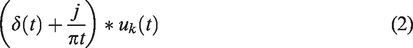
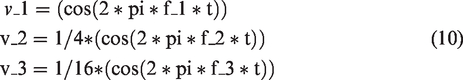
The overall framework of the VMD is a constrained variational problem. The VMD algorithm assumes that each modal component closely surrounds a certain center frequency, transforming the modal bandwidth determination process into a constrained variational problem, thereby separating the modal components through its solution. In the VMD algorithm, each component consists of a series of amplitude-modulated and frequency-modulated signals (AM-FM signals or modes), and its expression is given by
24

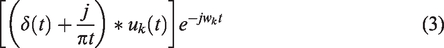
In the expression: Each mode undergoes a Hilbert transformation and calculates the analytical signal to obtain the unilateral spectrum corresponding to the component, given by
where, 2. Estimation of the center frequency 3. Calculating the square norm
where
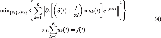
In order to solve the above variation problem, a penalty factor
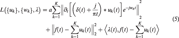
Iteration of
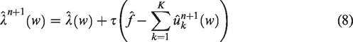
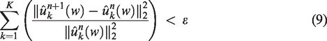
Iteration of the variational model is performed while the frequency center and bandwidth of each IMF component are updated until the iterative stopping condition is satisfied
The corresponding algorithm process can be described as follows:
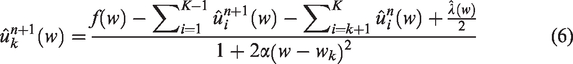
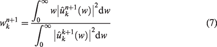
Initialization of According to the formulae (6) and (7) The noise margin parameter Repeat steps (2) through (3) until it can satisfy the iteration stop condition, then stopping iteration and obtaining the K IMF components.
When using the VMD algorithm for signal decomposition, it is necessary to manually set the number of decompositions in advance. The study found that in the decomposition, when

The signal
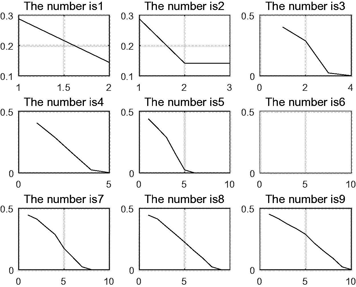
The average value of the instantaneous frequency of the component.
As seen from Figure 1, when K = 5, the curve bends largely downwards. This is because, to obtain the optimal solution for modality, the VMD algorithm searches the frequency domain in cycles. If the number of decompositions is too large, the component will break and flocculate, especially at high frequencies. This way, even at high frequencies, the average instantaneous frequency is lower, which is also the root cause of the downturn. If the decomposition continues, the signal will be destroyed, as shown in Figure 1(5), and the average instantaneous frequency drops rapidly. Therefore, the optimal decomposition number of the above signal is K = 4.
Flat wavelet denoising algorithm
Wavelet transform
25
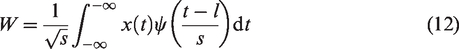
(WT) is a method that can analyze and transform locally in time (space) frequency, and can gradually multi-scale the signal (function) through the telescoping translation operation, and thereby achieving time division at high frequencies and frequency subdivision at low frequencies, which can automatically adapt to the requirements of time–frequency signal analysis. The expression of the wavelet transform is shown as follows. It can be seen as the sum of the whole signal

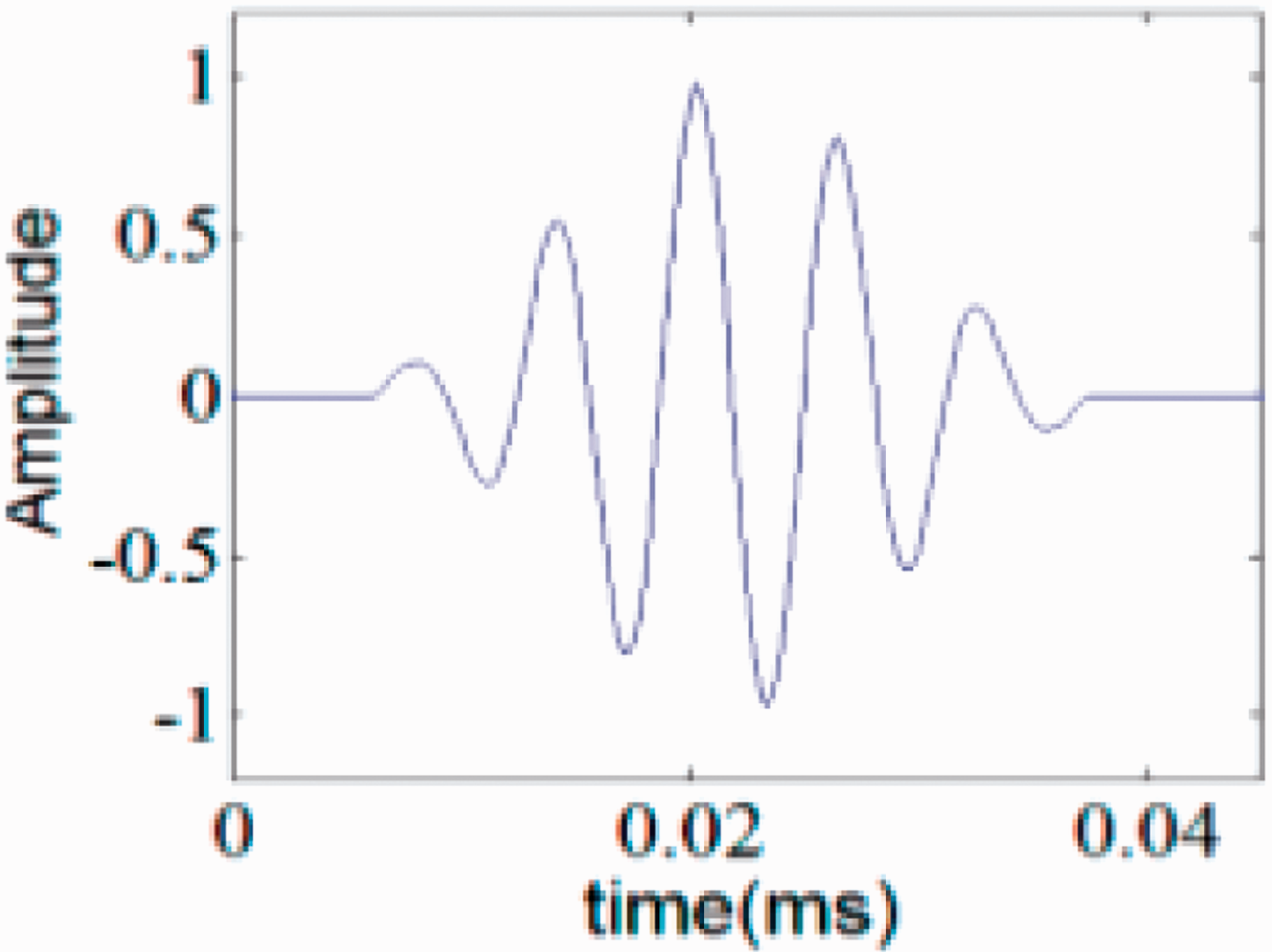
Five-cycle tone-burst.
Noisy signal is produced after wavelet transform, and the noise cannot be completely removed. But its wavelet coefficient has a strong correlation at each scale, especially in the vicinity of sudden change of the signal, and this correlation is more obvious. However, the noise-corresponding wavelet coefficients have no obvious correlation among the scales. Therefore, the correlation between the corresponding points of the wavelet coefficients at different scales can be used to determine whether the point is the signal coefficient or the noise coefficient, so that it can be chosen. 28 At the same time, after the noisy signal is denoised by the wavelet coefficient correlation, some noise corresponding wavelet coefficients may still remain in the vicinity of the signal mutation, so threshold denoising and smoothing processing are also required. Therefore, in this paper, we propose a cross-correlation threshold smoothing denoising algorithm based on wavelet correlation coefficients.
Consider a noisy signal,

Here,

Comparison of the absolute value of normalized correlation coefficient and wavelet coefficient is done, by which: if

Here, this paper refers to the threshold of noise level defined in Zhao et al.,
29
where
Flat variational modal decomposition
From ‘Variational mode decomposition’ section, it is seen that the IMF component obtained from the VMD method contains the main fault feature information. Spectrum analysis of the IMF component can effectively extract fault features. But the IMF component also contains a large number of noise signals. Under strong noise background, useful information may be submerged in frequency spectrum analysis of IMF components, thereby reducing the accuracy of fault diagnosis. To overcome these restrictions, in this paper, we propose a flat variational modal decomposition method based on wavelet coefficient correlation denoising. In FVMD, we applied the wavelet transform discussed in the previous section to IMFs during the shifting process just like the following equation
Obtain IMF according to VMD which has been discussed in ‘Variational mode decomposition’ section. The choice of the decomposition modulus K follows the method described in ‘Variational mode decomposition’ section. The flat wavelet coefficients are calculated according to the mother wavelet based on tone-burst signal and the smoothing denoising method described in ‘Flat wavelet denoising algorithm’ section
where 3. The threshold denoising method described in ‘Flat wavelet denoising algorithm’ section’ is used to perform threshold filtering on the wavelet coefficients in step (2), to filter out the noise signal near the signal mutation and obtain smooth wavelet coefficients 4. Reconstruct FIMF from the smooth coefficients through the inverse wavelet transform. 5. The regression coefficient between the FIMF component and the original signal in step (4) is calculated and the FIMF with a higher correlation coefficient is selected to reconstruct signal. Then, the reconstructed signal is used as the original signal to perform VMD, and the envelope spectrum analysis of the decomposed FIMF is performed so as to clearly extract fault information.
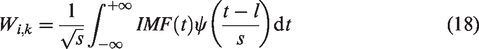
The FVMD-based fault diagnosis process can be represented as a flowchart as shown in Figure 3.
Flat variational modal decomposition algorithm fault diagnosis process.
Experiment analysis
Data collection
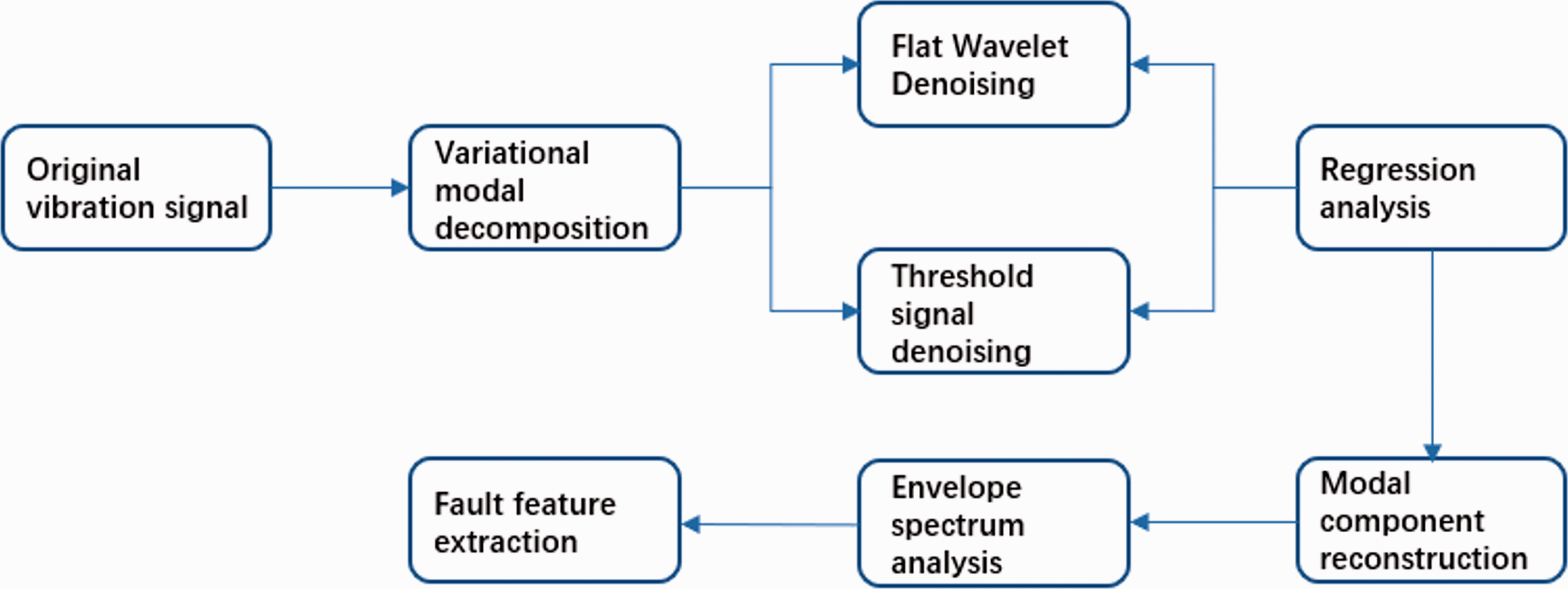
In order to verify the validity of the method proposed in this paper for the analysis of measured vibration signals, we analyzed a rolling bearing fault signal of inner ring and outer ring. The experimental data for bearing were provided by the Case Western Reserve University. The experimental equipment is shown in Figure 4. This experiment takes the bearing of the motor drive end as the diagnostic object. Single point damage is introduced into the inner ring and outer ring of the test bearing by means of electro discharge machining to simulate the three faults of the bearing. with fault diameters of 0.1778 mm, depth of 0.2794 mm, the data acquisition system consists of an acceleration sensor mounted on the upper side of the motor drive end with a sampling frequency of 12 kHz per channel. The motor speed was 1797 r/min and the length of the sample was 10240. In Ali et al., 8 there is a detailed description about the experimental data collection. In this study, we only consider the bearing states covering outer race fault (ORF) and inner race fault (IRF). The rolling bearing inner ring damage fault characteristic frequency is f1 = 162 Hz, and the outer ring damage fault characteristic frequency is f2 = 107 Hz. Their time domain waveforms and frequency domain waveforms are shown in Figure 5.
American West Reserve University bearing fault diagnosis test system.
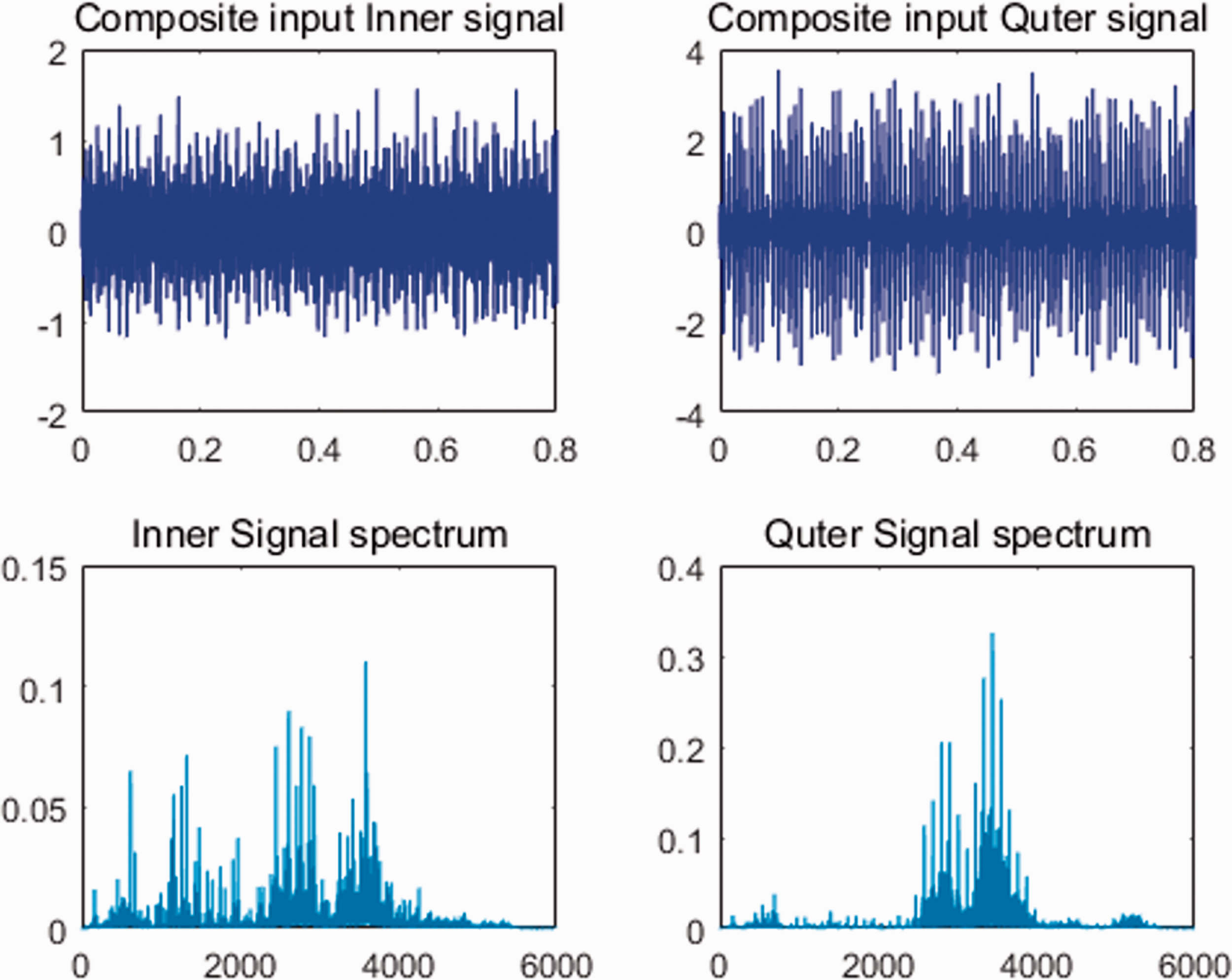
Input signal composition and its spectrum.
In this paper, the performance of FVMD algorithm is analyzed from the aspects of signal decomposition effect and signal de-noising, and the effectiveness and superiority of the FVMD method are illustrated by comparison with the EMD and the VMD methods.
Experiment with the proposed method
When FVMD is employed to decompose signals, first we must set three parameters, which are the balancing parameter of the data-fidelity constraint D, decomposing mode number K and time-step of the dual ascent W. In this study, D was set with the default value 2000, while W was set as 0.1 to avoid distortion. 31 The decomposition modulus K was chosen according to the method described in ‘Variational mode decomposition’ section. The inner ring fault signal is selected to perform VMD decomposition with 10,240 signal points. The mean value of the instantaneous frequency of the components under different K values is shown in Figure 6.
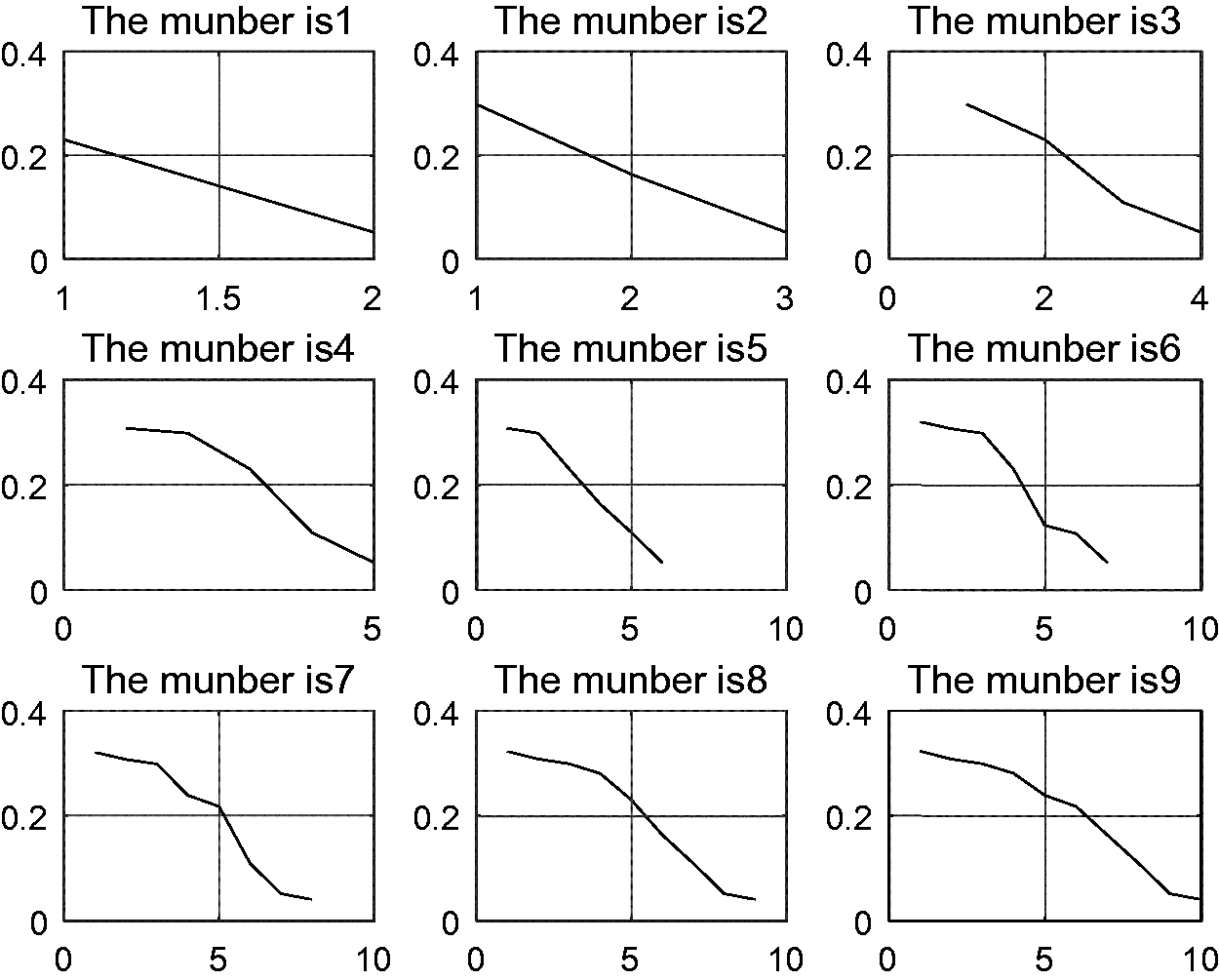
The average value of the instantaneous frequency of the Input signal.
Starting from K = 5, the mean value curve of the instantaneous frequency of the component decreases rapidly. This paper considers that over-decomposition has occurred. Therefore, the modal number is selected as 4. The fault signal of the outer ring and the inner ring of the rolling bearing is decomposed by VMD in the time domain as shown in Figure 7.
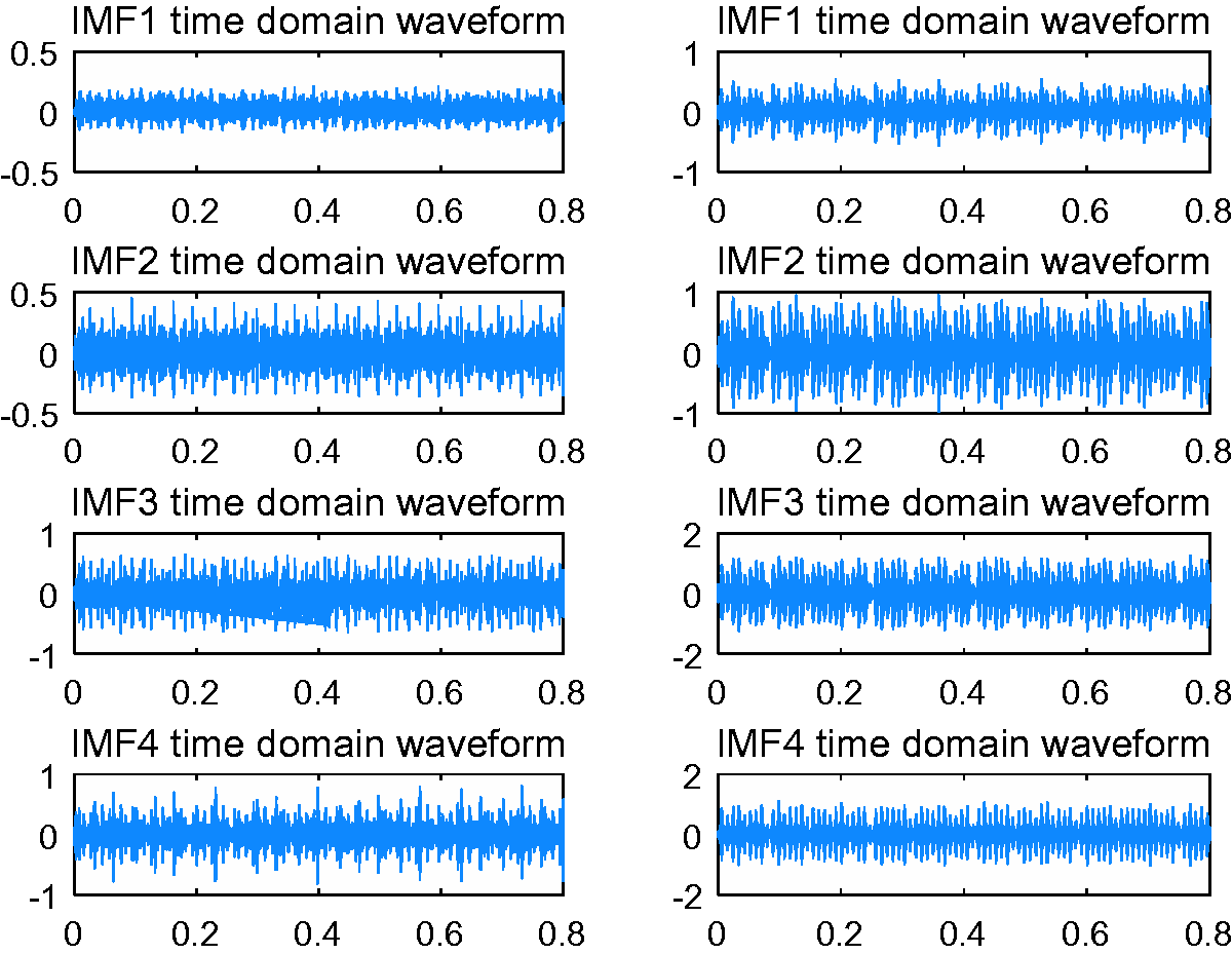
Time domain spectrum of each modal component after VMD processing. (a) Inner ring. (b) Outer ring. VMD: variational modal decomposition.
It can be seen from the time domain diagram that the signal decomposed by the VMD method has impulse components, and the periodic characteristics are not conspicuous, In addition, there is still a lot of noise interference, and the state information of the bearing is basically submerged. Therefore, the useful bearing state information cannot be obtained through the time domain waveform. The signal is further enveloped for spectral analysis, and the results are shown in Figure 8. Although there is a frequency component
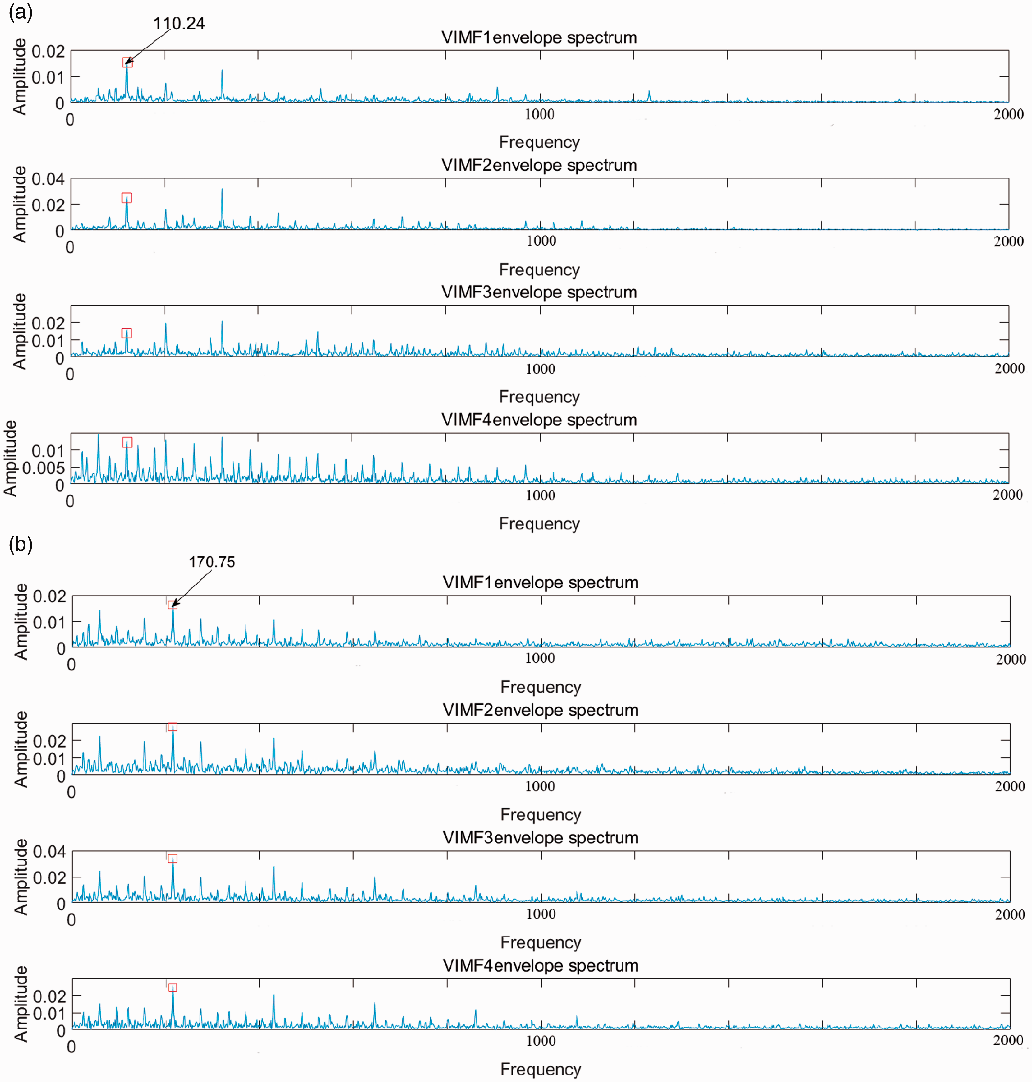
Envelope spectrum of each modal component after VMD processing. (a) Inner ring. (b) Outer ring. VMD: variational modal decomposition.
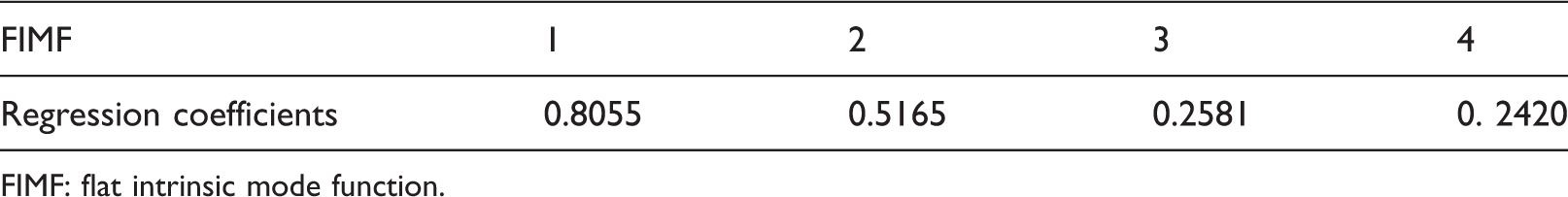
The signal is analyzed using the proposed method. First, the modal parameter is set using the component instantaneous frequency index, and the number of decomposition modes is determined to be 4. Then the parameters D and W are set using the VMD method to process the measured signal to obtain four IMF components. Then, the four IMF components are smoothened and denoised by the proposed method to obtain the smoothened FIMF. In order to ensure that the reconstructed signal can retain more information, finally, the regression coefficients of each FIMF component and the original signal after smooth denoising are calculated and the results are shown in Tables 1 and Table 2, and for the regression coefficient calculation method, the reader is referred to the algorithm in Montoril et al. 32
Regression coefficients of each component of the inner ring.

FIMF: flat intrinsic mode function.
Regression coefficients of each component of the outer ring.
FIMF: flat intrinsic mode function.
As shown in Tables 1 and 2, the regression coefficients of IMF1 and IMF2 are large, indicating that they retain the most significant characteristics in the original signal. So, these two IMF components are extracted for original signal reconstruction, which are decomposed and executed by the VMD. The envelope spectrum analysis was performed and the results are shown in Figure 9.
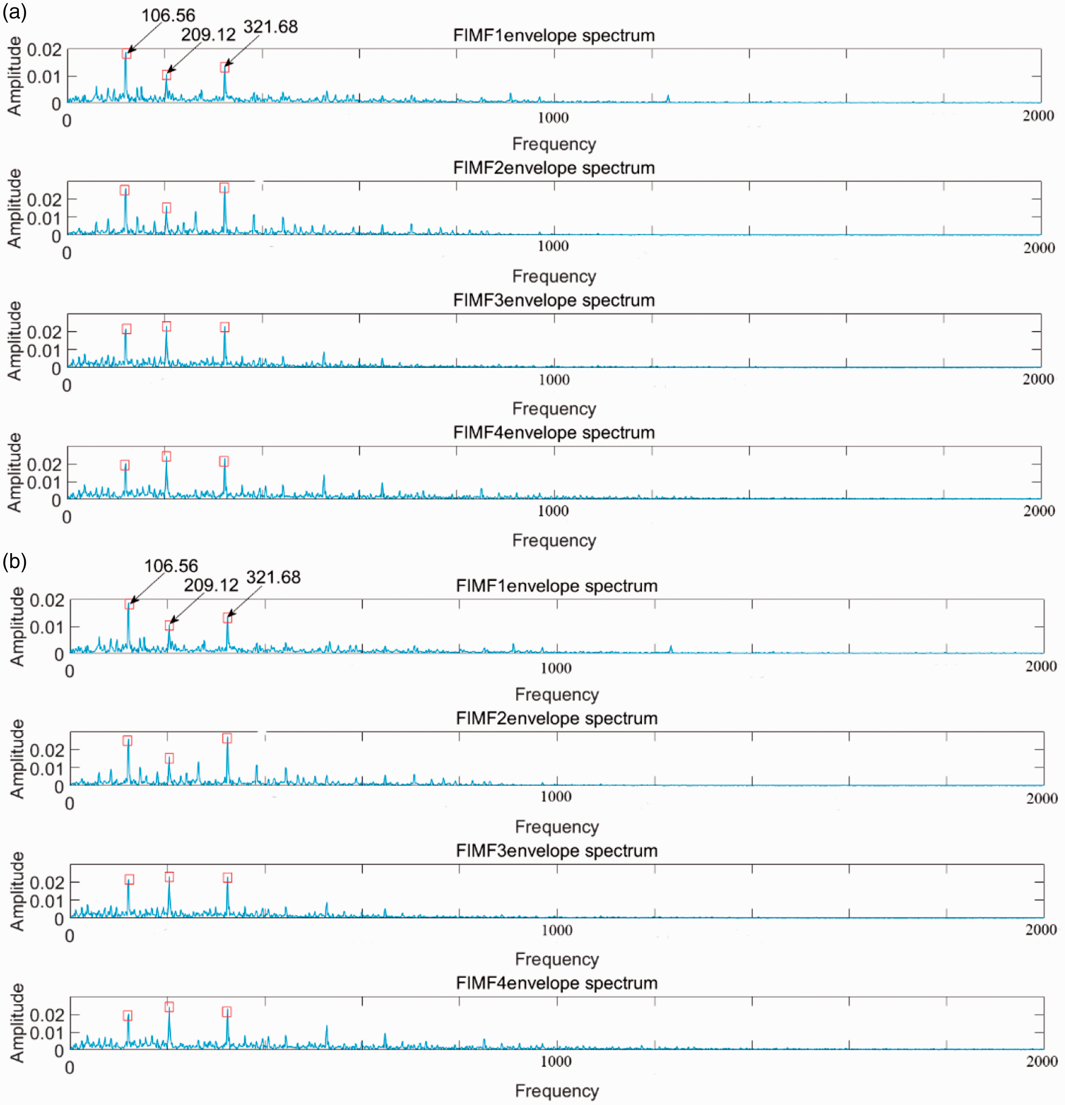
Envelope spectrum of each modal component after FVMD processing. FVMD: flat variational modal decomposition.
As shown in Figure 9, Figure 9(a) corresponds to the inner ring fault of the rolling bearing. Figure 8(a) shows a peak at 163.83 Hz, which is closer to the inner ring fault 162 Hz, and multiplier generation occurs, which is attributed to the correctness of the inner ring fault. It can be seen from Figure 9(b) in the bearing outer ring fault that a peak appears at 106.56 Hz, which is closer to the bearing outer ring fault frequency 107 Hz, and multiplier generation occurs here too, indicating that the bearing outer ring is faulty. It can be seen from the figure that after FVMD algorithm processing, the noise of the original signal is basically removed, and the fault information can be obviously extracted. Furthermore, there are local defects on the rolling elements of the bearing, and the analysis results are completely consistent with the actual situation. The actual diagnosis shows that the method in this paper can effectively remove redundant noise interference and ensure accurate fault diagnosis.
In order to verify the advantages of the method described in this paper, the EMD method and the VMD method are compared. In order to facilitate the comparative analysis, we take only the first four components after EMD and VMD processing.
It can be seen from the spectrum of EMD analysis (as shown in Figure 10) that there is a certain aliasing of the frequencies of the EMD components, which may cause the feature information to be decomposed into different modal components, so that it is submerged in the noise and weak fault information cannot be obtained. Therefore, the EMD method cannot completely remove the influence of noise and has some disadvantages. In the envelope spectrum of EMD which is shown in Figure 11, the frequency doubling of the first and the second components in the EMD decomposition signal is very obvious, but it also contains other frequency components and is accompanied by noise interference. The characteristic line is subtle. Using FVMD, the 162 Hz and the 107 Hz lines can be quickly found, which are consistent with the fault frequency of the inner and the outer rings of the bearing.
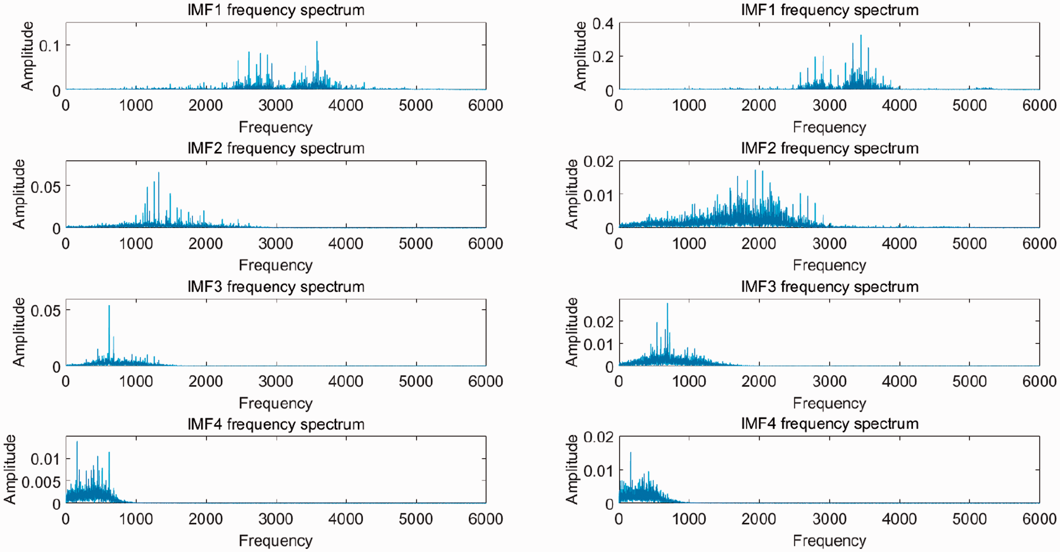
Spectrogram of each modal component after EMD processing. EMD: empirical mode decomposition.
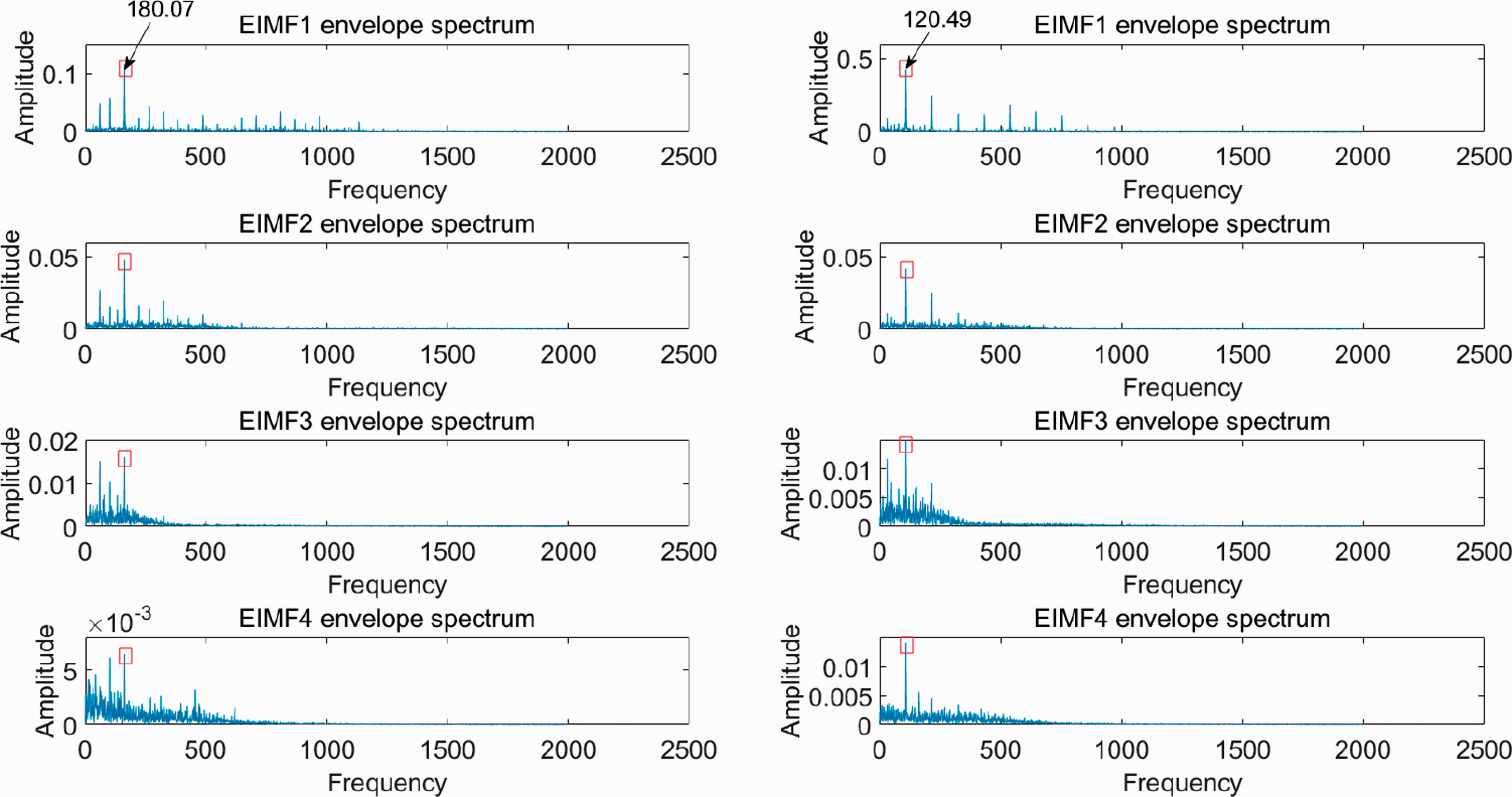
Envelope spectrum of each modal component after EMD processing. EMD: empirical mode decomposition.
In order to quantitatively analyze the denoising effect of the signal after noise reduction in the above two methods, the kurtosis value and the signal-to-noise ratio are selected as the evaluation indices after noise reduction. The kurtosis value indicates the fault characteristic information contained in the reconstructed signal. The larger the absolute value of the kurtosis index is, the higher the number of components containing the fault impact in the IMF, and the easier it is to extract more fault information. The signal-to-noise ratio reflects the denoising ability of the signal. The larger the signal-to-noise ratio, the better the denoising effect. The kurtosis values of the modal components after the fault signal has been denoised by the three methods are shown in Tables 3 to 5.
The kurtosis value of each modal component after EMD processing.
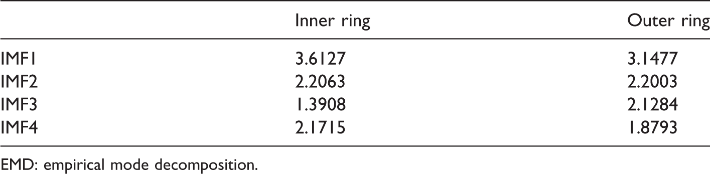
EMD: empirical mode decomposition.
The kurtosis value of each modal component after VMD processing.
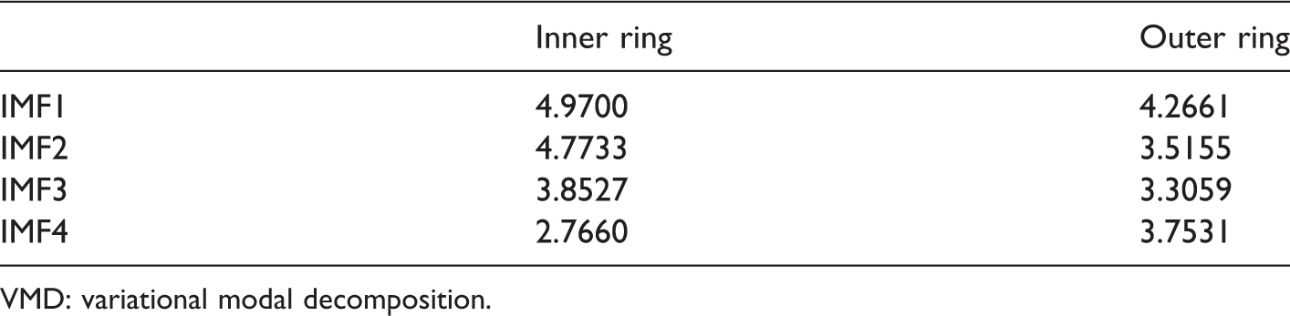
VMD: variational modal decomposition.
The kurtosis value of each modal component after FVMD processing.
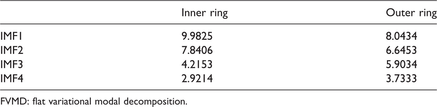
FVMD: flat variational modal decomposition.
It can be seen from Table 3 to 5 that after the original fault signal is processed by the FVMD method, the kurtosis values of the modal components are significantly higher than the EMD method and the VMD method, indicating that the FVMD method can effectively remove noise interference and retain more multiple original fault information. It can be seen from Table 6 that the signal-to-noise ratio of the signal after the FVMD processing has been significantly improved. Compared with the EMD and the VMD methods, the signal-to-noise ratio has increased by 77% and 44%, respectively, proving the effectiveness of the FVMD method.
Comparison of signal-to-noise ratio after denoising.
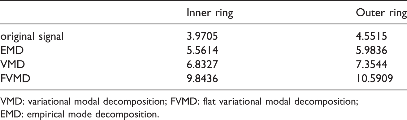
VMD: variational modal decomposition; FVMD: flat variational modal decomposition; EMD: empirical mode decomposition.
In order to make the results more convincing, we selected the fault signal under different working conditions for FVMD, EMD and VMD experiments, and calculated the kurtosis value of the reconstructed signal and the signal-to-noise ratio of the reconstructed signal after denoising. The results are shown in Tables 7 to 10.
Inner ring signal-to-noise ratio at different speeds.
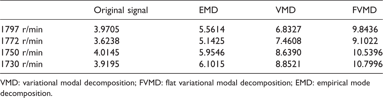
VMD: variational modal decomposition; FVMD: flat variational modal decomposition; EMD: empirical mode decomposition.
Outer ring signal-to-noise ratio at different speeds.
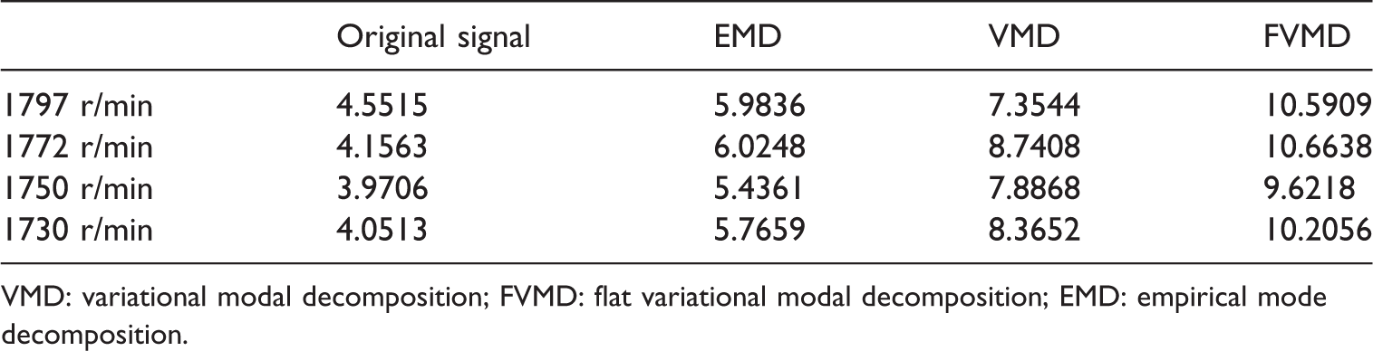
VMD: variational modal decomposition; FVMD: flat variational modal decomposition; EMD: empirical mode decomposition.
The kurtosis value of the inner ring reconstruction signal at different speeds.
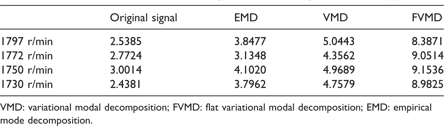
VMD: variational modal decomposition; FVMD: flat variational modal decomposition; EMD: empirical mode decomposition.
The kurtosis value of the outer ring reconstruction signal at different speeds.
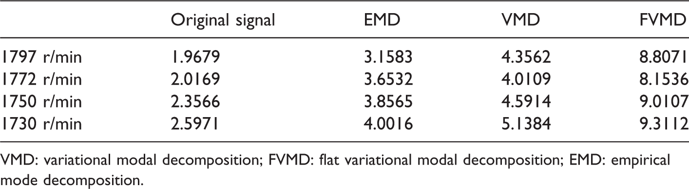
VMD: variational modal decomposition; FVMD: flat variational modal decomposition; EMD: empirical mode decomposition.
It can be seen from Tables 7 and 8 that at different speeds, the signal-to-noise ratio of the original signal has been significantly improved after being processed by the FVMD method, and is 77% higher than the EMD algorithm and 44% higher than the VMD algorithm. This indicates that the FVMD method can effectively remove noise interference. At the same time, it can be seen from Tables 9 and 10 that at different speeds, the kurtosis value processed by FVMD algorithm is much higher than that of EMD and VMD algorithm, indicating the FVMD method can retain the fault information in the original signal while removing noise interference. Thus, the superiority of the FVMD algorithm in noise reduction is verified by comparison with EMD and VMD algorithms.
Conclusion
Considering the susceptibility of vibration signal-to-noise interference, which may cause the normal signal to be submerged in the interference, in this paper, we proposed a new smoothing denoising algorithm based on the traditional VMD algorithm. In this paper, the smoothing wavelet operator is designed and innovatively introduced into the decomposition process in the process of VMD decomposition. In the traditional VMD decomposition process, the fault signal is denoised by the construction of a new set of mother wavelets, and the threshold signal denoising method is used to process the noise at the signal mutation to obtain the FIMF. Then, by calculating the regression coefficient, the FIMF component was selected to reconstruct the new signal, and then the signal was de-noised by performing the VMD decomposition again. The algorithm is applied to the bearing fault diagnosis experiment and compared with the traditional EMD and VMD algorithms. The simulation results show that the proposed algorithm has a significant improvement in signal-to-noise ratio after denoising, compared with the traditional algorithm. The signal-to-noise ratio of the original signal has been significantly improved after being processed by the FVMD method, which is 77% higher than the EMD algorithm and 44% higher than the VMD algorithm. Simulations and experimental results have proved the effectiveness of the proposed method in this paper. In terms of application prospect, the smooth wavelet designed in this paper can be applied to a variety of complex objects. For different signal types, the algorithm in this paper can be tried to be extended to a broader field.
Footnotes
Data availability
Data from this manuscript may be made available upon request to the corresponding author.
Declaration of conflicting interests
The author(s) declared no potential conflicts of interest with respect to the research, authorship, and/or publication of this article.
Funding
The author(s) disclosed receipt of the following financial support for the research, authorship, and/or publication of thisarticle: This study was supported by the Basic Research Projects for Colleges and Universities of Liaoning Province(LJZ2017035); Science and Technology fund of Liaoning Province (20180550002); Liaoning Province Key Research and Development Project(2017225016);National Science Foundation of China (51705341).