
Abstract
In recent years, the opposed high-speed gas bearing system has been gradually valued and used in the field of precision machinery, especially for precision instruments and mechanisms requiring high speed, high precision, and high rigidity. Although the bearing capacity is not as good as the oil film bearings, it can provide a working environment where the rotor can generate high speed and low heat without deformation of the shaft, and the gas pressure distribution of clearance in bearing also has better stability. Due to the strong nonlinearity of the gas film pressure function of gas bearings and the fact that the actual shaft system possesses dynamic problems including critical speed, spindle imbalance or improper bearing design, it will cause the rotation process of the shaft to produce a nonperiodic motion and instability, and even chaotic motion under certain parameters. And these irregular movements can even cause machine damage or process delays when serious, so in order to understand the process of working under the conditions where the system will have a nonperiodic phenomenon and to avoid the occurrence of irregular vibration especially chaos. In this paper, the opposed high-speed gas bearing system feature will be discussed in detail with three different numerical analysis methods, i.e. the finite difference method, perturbation method, and mixing method. The relevant theories include dynamic trajectories, spectrum analysis, bifurcation diagram, Poincare map, and the maximum Lyapunov exponents. From the results of nonlinear dynamic behavior of the rotor center, periodic and nonperiodic motions occur at different rotor masses and bearing parameters, respectively. Especially, for the chaos of shaft exists at specific intervals and can be distinguished efficiently. Meanwhile, it is found to ensure that the bearing system can suppress the phenomena of chaos actively by adjusting the bearing parameters, and reduce the system loss caused by irregular vibration. It is expected to be an important basis for designing a precision shaft or mechanism and to enhance the stability and performance of bearing system.
Introduction
Nowadays, ultra-precision machining and measuring technologies for precision instruments and equipment components have been further developed to the nanometer level. In addition to the substantial increase in measurement accuracy requirements, the need has arisen for nanometer-scale displacement and positioning, such as precision processing machines and semiconductor wafer cutting machines, high-speed hard drives, etc. Besides, a system in need of clean, ultra-high speed, accurate positioning also has a large number of applications.1,2 In order to meet the relevant requirements, such as requiring the rotation accuracy of the gauges to reach the nanometer level, and requiring the maintenance of a high degree of stability, the application of the opposed high-speed gas bearing system among the key components is gaining more and more attention. For example, the high accuracy supporting techniques for gyro motor becomes increasingly using the opposed high-speed gas bearing to replace the mechanical bearing, and performs higher stiffness, longer life and higher precision. Gyroscopes applied opposed high-speed lubrication bearing of gyro motor is currently the highest precision gyroscope. Especially for the wedge-shaped type of opposed high-speed gas bearing, it could work in high speed, high structure stability, strong anti-overload ability, good and centroid stability, etc. 3 In the research on gas bearings, how to accurately calculate the gas film pressure distribution has always been an important issue. Nguyen et al.4–6 has proposed to solve the gas bearing pressure distribution problem of complex boundaries, using the finite element method (FEM) after 1991. In contrast, the opposed bearings studied in this paper have grooves on their surface, and the related research in this area is quite rare. In 1958, Whipple 7 was the first to study the characteristics of gas bearings for herringbone grooves. Vohr 8 studied gas bearings with helical grooves in 1963 and deduced the differential equation of the gas film pressure on the assumption that the number of grooves is close to infinity. This theory is called “Narrow Groove Theory”. Until 1991, Absi and Bonneau 9 used the FEM to solve the pressure distribution function of herringbone bearings and studied their related characteristics, including stability analysis, pressure distribution, and the influence of key parameters on the system. It can be seen from the above literature that the gas film dynamic characteristics of gas bearings have a great influence on the entire bearing support system, especially the pressure of the gas film, the rigidity of the gas film, and the damping effect. In the literature of the rotor dynamic behavior, in 1974 it was found by Bently 10 through experimentation that a rotor bearing system has subharmonic vibration of order 2 and order 3. Choi and Noah 11 then used the analytic method to prove the existence of subharmonic vibration in rotor bearing systems.
Recently, many electromechanical and opto-electric devices are downsizing and printed-circuit boards used in these devices have also been made smaller and smaller. So, the diameters of the small holes for fixing electric parts to the printed-circuit board had to be reduced. Opposed conical bearings with spiral grooves were designed for a high-speed spindle to drill these small holes in printed-circuit boards. Compared with oil bearings, opposed conical bearing system has much lower power consumption at high speeds and without causing environmental problems. Moreover, opposed conical gas bearing has a larger load capacity than aerostatic bearings, as a higher supply pressure can be used to suppress the rotor instability. About the research of this gas bearing, in 1972, Kazimierski 12 studied the conical (wedge-shaped) gas bearing system and considered the rotor dynamic behaviors mounted in two hybrid conical gas lubricated bearings. It was found an optimum angle of conical gas bearings gives the maximum stability of the motion of the rotor with respect to the self-excited, cylindrical vibrations is important and can be obtained. Meanwhile, the existence of an optimum stiffness of elastic elements of support with respect to the creation of self-excited whirl vibrations of the rotor and foundation is proved. In 2002, Yoshimoto et al. 13 applied the conical bearings with spiral grooves for high-speed spindles to investigate the performance of bearing system theoretically and experimentally. They first presented these bearing types for pressurized water fed to the inside of the rotating shaft and then introduced into spiral grooves through holes located at one end of each spiral groove. The stability of the proposed bearing was also theoretically predicted by the perturbation method, and the numerical results were compared with experimental results. In 1993, Agrawal 14 studied the power-shaped multipad hydrodynamic conical gas bearings working in a compressible fluid that is suitable for high speed turbomachines. The results revealed that the bearing has higher load capacity both in the radial and axial directions than traditional aerostatic bearings. Especially, the radial load is three times that of an axial groove bearing under high rotational speed. This conical gas bearing is more stable and the friction factor is about one-third that of an axial groove bearing. It is concluded that the radial load is approximately a function of compressibility number and eccentricity only, and the axial load is approximately a function of compressibility number only. In 2007, Pan et al. 15 presented the five degrees-of-freedom characterization of the stability of a conical gas bearing with the spiral-groove design for bearing numbers up to 500. The stability thresholds of bearing system with respect to each mode including axial, cylindrical, and conical modes are analyzed as functions of the bearing number and rotor mass, respectively.
Wang16,17 used a mixing method to solve the gas film pressure of high-speed rotor gas bearings and grooved gas shaft systems. At the same time, the dynamic action of the rotor and journal centers was analyzed by the trajectory, spectrogram, and bifurcation diagrams. The study shows that the rotor center and journal center have periodic, quasi-periodic, or sub-harmonic motion under different operating conditions. Subsequent applicants successively analyzed other gas shaft systems and found that the system may even occur nonlinear chaotic motion under certain operating ranges.18,19
In addition, in the related experiments, Young 20 used ultrasonic technology to detect abnormal rotation precision and spindle vibration instability produced by special operating conditions in 1992, but it was still in the experimental stage and lacked theoretical analysis and verification. There are still many scholars in the follow-up research, but most of them have focused on the discovery and experimental analysis of the abnormal vibration behavior of the oil film bearing system. There have only been a few developments on the experimental planning and testing platform technology for gas bearing systems. In 2002, Nikolaou 21 designed a test platform and performed spectrum analysis on the vibration and noise signals of the spindles supported by the ball bearings, and attempted to compare them with the theoretical values, but the effect was limited. In the Taguchi Experimental Planning Section, Wu and Kung 22 used the Taguchi method in 2005 for an experimental hybrid oil film bearing design test factor and level, containing the oil film viscosity, the amount of oil and orifice size, etc. to analyze normal and abnormal behavior of the rotor bearing operation, but it could not confirm whether this state is chaos phenomenon. In 2008, Al-Raheem 23 carried out anomaly diagnosis analysis of ball bearings through theoretical analysis, but it was still at the theoretical stage. However, the related research and development of the above-mentioned literature for opposed high-speed gas bearing systems is quite scarce and lacking in theoretical integration and verification. Therefore, integrating theoretical analysis technology will become an important direction for academic research and industrial production in the future, but it is still needed to do sustained research and development on the related theories. Today, with emphasis on speed and efficiency in production, to discuss shafting of high-precision and high stability, which is easy to detect has become an important research direction of contemporary industry and academia, and is also the main focus of this paper.
Research methods
This paper researches on the opposed high-speed gas bearing (OHGB) systems required for the precision machinery industry, especially suitable for ultra-high-speed areas and environments in need of a high load-carrying capacity. At present, the opposed-type bearing is a traditional H-type bearing structure, as shown in Figure 1. This type of bearing is a combination of plain thrust bearings and cylindrical journal bearings, sometimes referred to as “closed linear bearings”, which have matured to date and which have grooves in the bearing surfaces that produce a larger bearing ability. However, if the application has a tapered bearing surface or a spherical surface shaft, it is not suitable. For this purpose the present paper mainly studies two shafts, which are different from conventional bearings, comprising an opposed wedge-shaped gas bearing and an opposed dome gas bearing, in order to summarize the optimization design criteria for the opposed-type high-speed gas bearings.
H-type bearing structure: (a) spiral groove type; (b) herringbone spiral groove type.
Governing equations of opposed wedge-shaped gas bearings
Opposed wedge-shaped gas bearings have the ability to support radial and axial loads, and can be used in the support of contact surfaces with special needs. There are two main forms of application: opposed obverse wedge-shaped and reverse wedge-shaped bearings, with the structure shown in Figure 2.
Opposed wedge-shaped bearing structure: (a)obverse wedge shape; (b) reverse wedge shape.
Since the bearing system is mainly gas-fluid-supported, the following basic assumptions have to be fulfilled:
The flow of the gas film is in an isothermal, laminar flow state. The gas viscosity coefficient does not change with the pressure and temperature, as a constant.
Therefore, the compressible Reynolds equation of the gas film pressure is as follows

This type of bearing in the wedge-shaped body parameters includes a half cone angle of
Opposed wedge-shaped bearings analyzed in this study are often used industrially. For realistic operating conditions, thereby simulating and analyzing the dynamic performance of the gas film pressure and the rotor, the groove angle is set to 161.7º–162.7º.
The thickness of the gas film can be expressed in terms of


Solution of instantaneous gas film supporting force
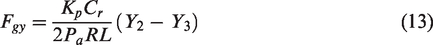
In Figure 1, the pressure distribution,

Rotor dynamic equations and computation procedure
The analysis presented in this paper considers a rotor-bearing system comprising a perfectly balanced, flexible rotor of mass mr supported symmetrically on opposed wedge-shaped bearings, which are mounted on rigid pedestals. With these idealizations, it is possible to consider one bearing in isolation. Hence, the system under investigation consists of a rotating rotor of mass mr with two degrees of translatory oscillation in the transverse plane. The idealized rotor-bearing model is shown in Figure 3, in which O1 is the geometric bearing center, O2 is the geometric rotor center, O3 is the geometric journal center,
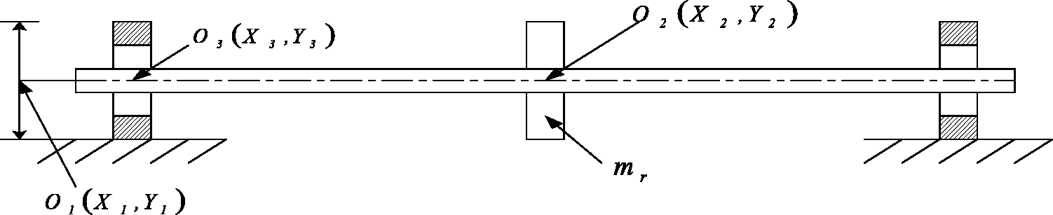
Model of flexible rotor supported by two gas bearings.
In the transient state, the equations of motion of O2 (i.e. the rotor center) can be written in Cartesian coordinates as


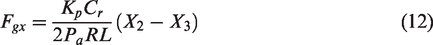
Regarding the journal center, O3, the resulting forces in the horizontal and vertical directions are as shown in Figure 3. From the equilibrium of forces, the forces applied to the journal center, O3, may be expressed as


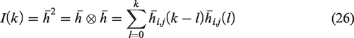
The following transformation is introduced
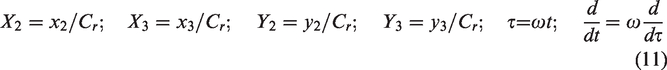
Additionally, the following nondimensional groups are defined
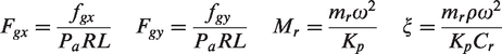
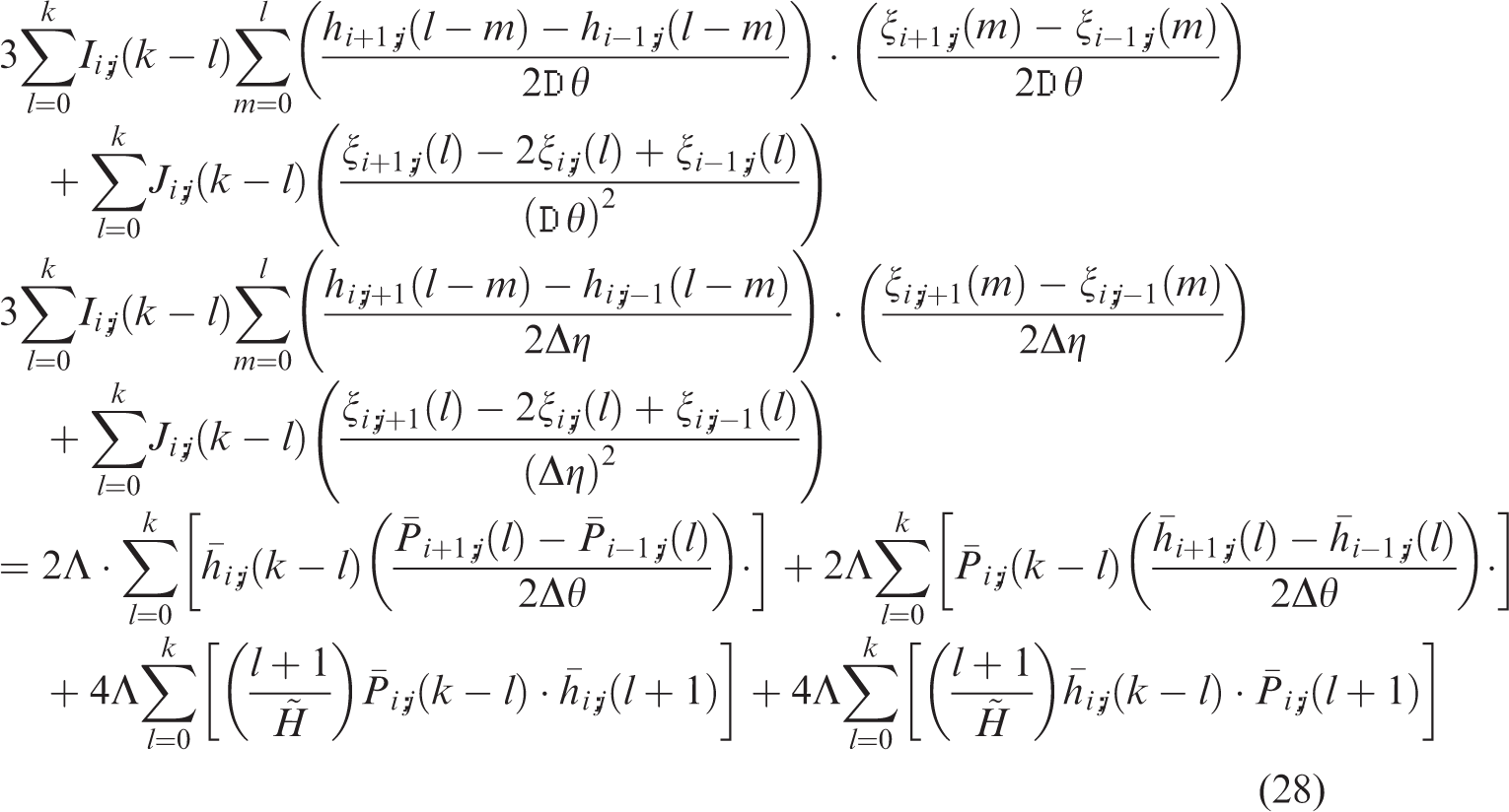
Substituting these nondimensional groups into equations (7) to (10) yields


Mathematical formulation of numerical simulation
In the model of the bearing, the Reynolds’ equation is a nonlinear partial differential equation, so a direct numerical method is used for its solution. To solve the bearing gas pressure distribution the perturbation method,
12
traditional finite difference method (FDM),
15
and a mixing method16,17 were used. For traditional FDM, let us first discretize equation (1) using the central-difference scheme in the
Then, the pressure distribution at each time step is obtained using an iterative calculation process from the above traditional numerical method.
In this paper, the mixing method is used and it is a combination of the differential transformation method (DTM) and the FDM. Differential transformation 19 is applied to deal with equation (1) and this method is also one of the most widely used techniques for solving differential equations due to its rapid convergence rate and minimal calculation error. A further advantage of this method over the integral transformation approach is its ability to solve nonlinear differential equations. The theoretical analysis is introduced in the following.
For the nonlinear Reynolds equation time domain, the DTM was first used to discretize the time into intervals and the central difference scheme of the FDM was then applied to the coordinates of the locations. The basic principle of the DTM is as follows.
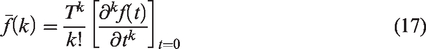
The differential transformation of the function of f(t) is defined as
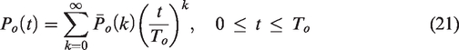
Calibration is needed to ensure precision during the calculation, therefore, when the second time interval is used, equations (19) and (20) are used to perform calibration
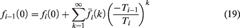
If
If the calculated values on each side of the equals’ signs in equations (19) and (20) vary greatly, precision is insufficient. Therefore, the time interval T needs to be reduced and re-calculation is necessary.
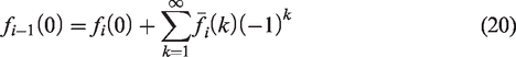
The basic arithmetic operation for the differential transformation is as shown in Table 1.
Basic arithmetic formula for the differential transformation.
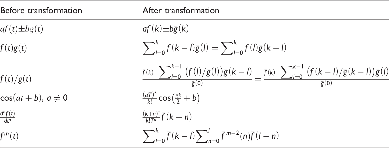
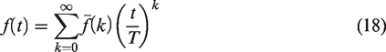
The differential transformation of the governing equation and the boundary condition are obtained and the pressure function theorem domain are divided into n number of sub-intervals, the pressure solution pf for each sub-internal is expressed as an inverse transformation equation. If the theorem domains of the sub-intervals are T0, T1, T2, T3, …, then the expression for the function in the first interval, based on equation (18), will be
If the initial value of 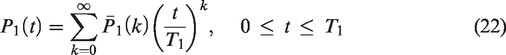
From 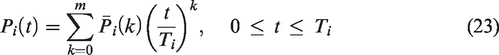
For solving the Reynolds equation for the current gas bearing system, the differential transformation method is used for taking transformation with respect to the time domain τ, and hence equation (1) becomes
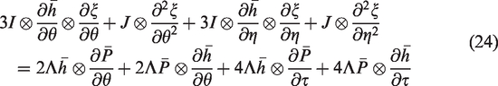

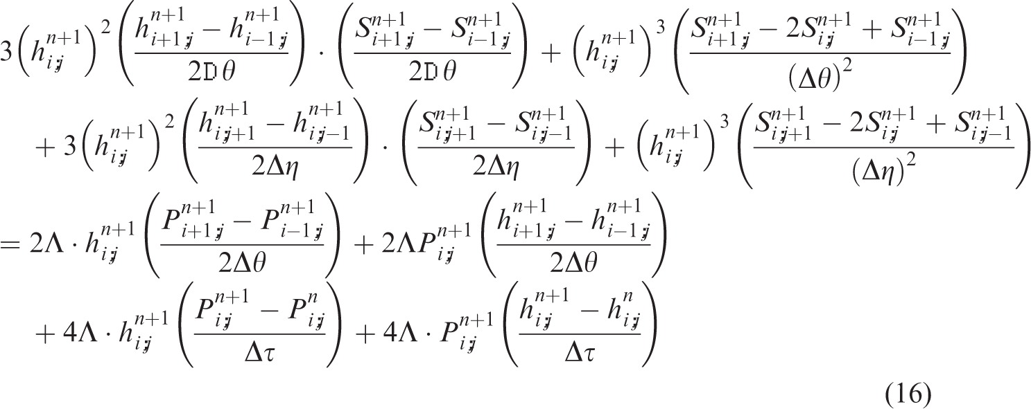
The FDM is then used to discretize equation (24) with respect to the θ and
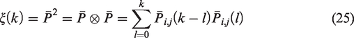
Substituting equations (25) to (27) into equation (24) yields
Computing the motions of the rotor center is an iterative procedure, which first determines the acceleration, then the velocity, and finally the displacement, step-by-step over time. The computation procedure begins by specifying an initial static equilibrium state. The initial displacement of the rotor (
The iterative computation procedure can be summarized as follows:
Step 1: Following a time increment
Step 2: The displacements of the rotor center obtained from Step 1 can then be determined and the corresponding change in the value of the gap (
Step 3: The pressure distribution obtained from Step 2 is integrated to estimate the internal force.
Step 4: The displacement and velocity values computed in Step 1, the pressure distribution calculated in Step 2, and the internal force obtained in Step 3 are taken as the new initial conditions. Using this new set of conditions, the calculation procedure returns to Step 1 to compute the changes in the gas bearing system during the time interval
These three steps allow determination of the pressure distribution, the relationship between the gas film thickness and change of position, variation of the gas film bearing force, and the dynamic orbits of the rotor, etc. at each time point. In addition, the maximum Lyapunov exponents can be used as a primary determination factor to predict periodic, quasi-periodic, aperiodic, and chaotic motion caused by such factors as the bearing number, mass of the rotor, and so on. By using the bearing number and the rotor mass of the air bearing as bifurcation parameters, a full view bifurcation diagram can be constructed. An analysis of stability can be conducted and the relationship between the maximum Lyapunov exponents and each of the previously mentioned factors can be interpreted. The parameters of the stable and the nonstable region of the system can be determined.
To further verify the accuracy of the numerical analysis, two different numerical methods were used (as previously mentioned) to ensure that the mixing method proposed in this paper was applicable and to increase the calculation precision.
Rotor dynamic analysis
In this study, the time series data of the first 1000 revolutions are excluded from the dynamic behavior investigation so as to ensure that the data used represent steady-state conditions. The resulting data include the orbital paths and velocity of the rotor center O2 and the orbits of the journal center O3. These data are used to generate the power spectra, Poincaré maps, and bifurcation diagrams.
Poincaré map
A Poincaré section (map) is a hypersurface in the state space that is transverse to the flow of a given dynamic system. In nonautonomous systems, a point on the Poincaré section is referred to as the return point of the time series at a constant interval of T, where T is the driving period of the exciting force. The projection of a Poincaré section on the X(nT)-Y(nT) plane is referred to as the Poincaré map of the dynamic system.
Power spectrum
The power spectra for the vertical and horizontal displacement of the journal center O3, and the rotor center O2, are obtained by using fast Fourier transformation to show the spectrum components of the motion. In this paper, the frequency axis of the power spectrum plot is normalized by using the rotor mass and rotational speed.
Bifurcation diagram
To generate a bifurcation diagram, the rotor mass (or speed) is varied with a constant step, and the state variables at the end of the integration process are used as the initial values for the next mass (or speed). This means that there is a tendency for the integration to follow a single response curve. Variation of the X(nT) and Y(nT) coordinates of the return in the Poincaré map with rotor mass(or speed) is then plotted to form the bifurcation diagram.
Results and discussion
Dynamic analysis of the bearing system with the results of different numerical methods
For the OHGB system, three different numerical methods including the FDM, perturbation method, and proposed method are used to compare the numerical simulation results for opposed wedge-shaped bearings (opposed obverse wedges and opposed reverse wedges). The result shows the proposed mixing method binding DTM and the FDM, the traditional FDM and perturbation method
12
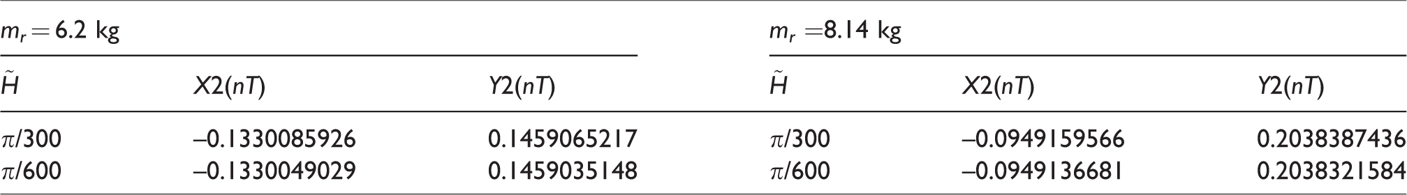
have a better fit when the rotor has a large mass. This also shows that the mixing method raised in this paper reveals higher accuracy and better convergence than the other methods with respect to different time steps and different opposed wedge-shaped bearings. The comparison of rotor center trajectory values on Poincaré map (X2(nT) vs. Y2(nT)) is as shown in Table 2 and the behaviors of rotor center with specific operational parameters are all periodic motions. Then the simulation results in Table 2 can be compared objectively and the differences were observed by three numerical methods. For numerical stability analysis, the impact of the different time steps is studied and the displacement changes are compared under different operating conditions by the numerical value of the Poincaré section, as shown in Table 3. From Tables 2 and 3, DTM and FDM (mixing method) is applied to obtain the dynamic orbits under different operating parameters for the OHGB system. For different values of the time step
Comparison of opposed wedge-shaped bearings (the opposite obverse wedge shape and opposite reverse wedge shape) system for rotor center displacement on Poincaré map with various numerical calculations.
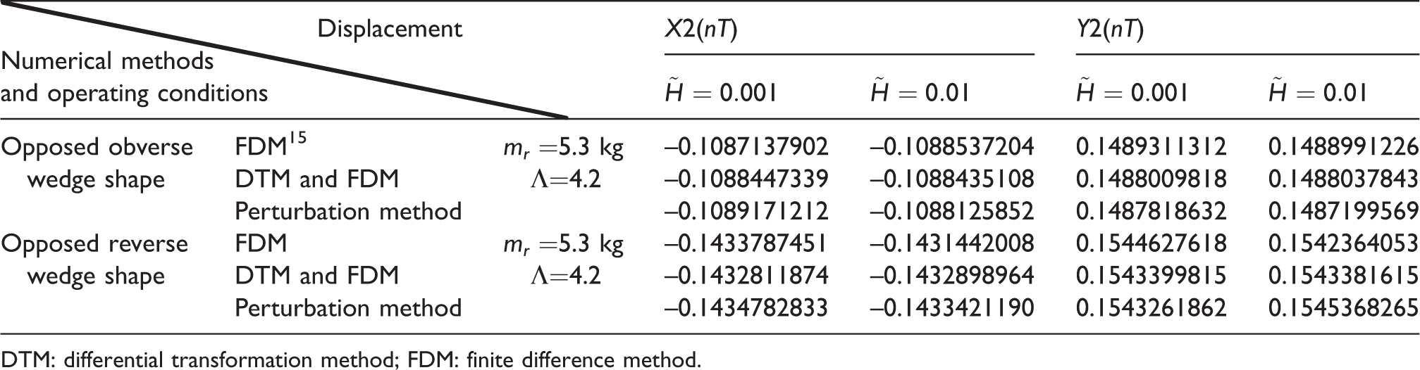
DTM: differential transformation method; FDM: finite difference method.
Poincaré map numerical comparison for different time steps
For the grid number analysis, the traditional FDM, perturbation, and mixing methods are used to solve equation (1) with uniform mesh size. Meanwhile, the three methods are calculated and compared with different values of the mesh size in space. It can be seen that the rotor center performs four decimal places by mixing method (DTM and FDM) better than the traditional FDM and perturbation method with different amount of grids shown in Table 4 (in the revised paper). It can also be seen that the rotor orbits are in agreement to approximately four decimal places for the different mesh sizes obtained by DTM and FDM at the values of bearing number (Λ = 4.2 and 7.1) as shown in Table 4.
Comparison of Poincaré maps of rotor center with different values of Λ and mesh size by FDM, mixing method, and perturbation method (time step: 0.01, mr =5.3 kg).
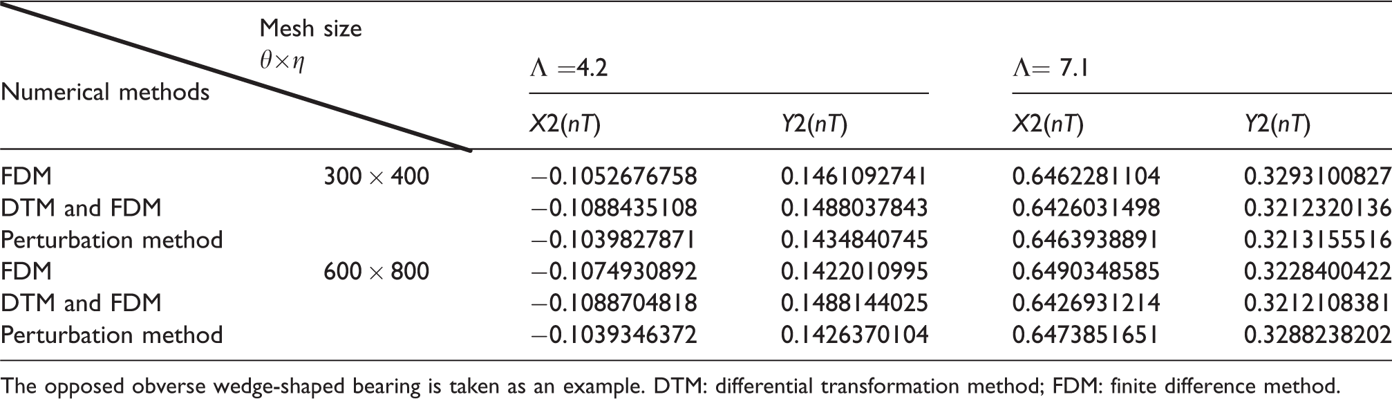
The opposed obverse wedge-shaped bearing is taken as an example. DTM: differential transformation method; FDM: finite difference method.
From the above numerical results, it can be seen that the mixing method of this study has the best accuracy than FDM and perturbation method. Meanwhile, it has better applicability for this OHGB system. Whether for different opposed-type bearings, the system trajectory can be calculated effectively and accurately by the mixing method. At the same time, in order to shorten the bifurcation characteristics of the subsequent calculation, the test results in Tables 2, 3, and 4 show that the simulations with sufficient accuracy can be obtained without too small time steps and too many grid numbers. Therefore, in the subsequent dynamic analysis section, π/300 is taken as a time step and 300 × 400 is taken as a grid number to calculate.
Rotor dynamic behavior analysis of the gas bearing system
Rotor impact on the system
Take the opposed obverse wedge-shaped bearing as an example, the bearing number in the system is (rotational speed) Λ = 4.5, and the mass of the rotor mr is taken as a bifurcation parameter.
Dynamic trajectories map
From Figure 4.1(a), (b), 4.2(a), (b),…, 4.6(a), (b) it can be observed that under the case of the lower mass of the rotor center and of the journal center (mr =5.3 kg), the trajectory shows the regular pattern, and when the mass raises to mr =6.98 kg, the nonperiodic phenomenon replaces the regular motion. At the same time when the rotor mass has reached mr =7.71 and 8.11 kg, the dynamic trajectory continues the cycle and the sub-cycle movement, but this cycle is in response to mr =8.25 kg, and then turns into nonperiodic motion. And when mr =9.39 kg, the bearing system remains unstable with nonperiodic behavior.
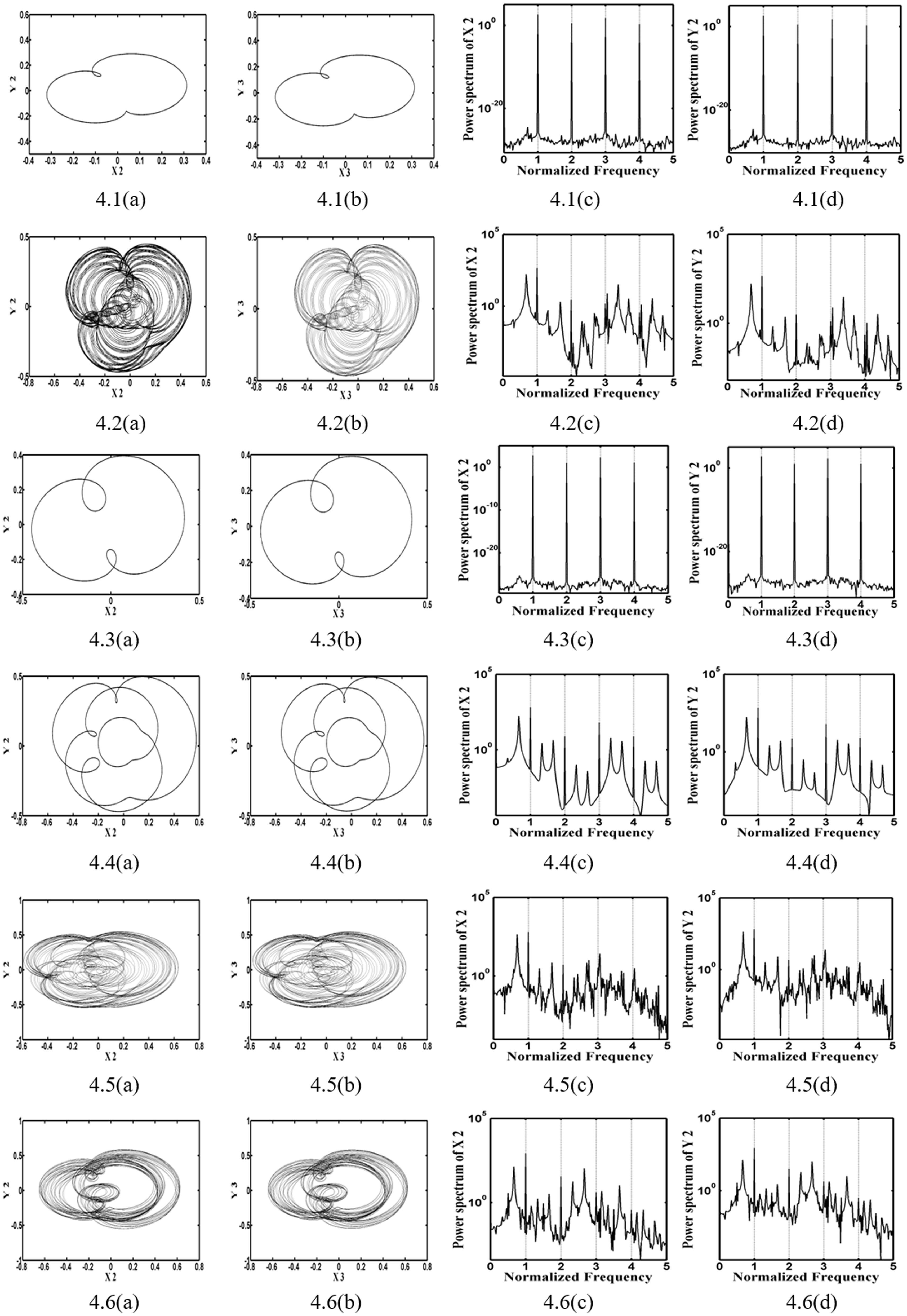
The dynamic trajectory (Figure 4.1(a) to 4.6(a)) of the rotor center when the rotor mass is mr = 5.3, 6.98, 7.71, 8.11, 8.25, 9.39, phase plan (Figure 4.1(b) to 4.6(b)), spectral response of the center of the rotor in the horizontal direction (Figure 4.1(c) to 4.6(c)), and the vertical direction (Figure 4.1(d) to 4.6(d)), the system bearing number is Λ = 4.5.
b. Spectrum analysis chart
Figure 4.1(c), (d), 4.2(c), (d),…, 4.6(c), (d) shows the dynamic response of the rotor center in the horizontal and vertical directions. The studies show when the rotor mass is mr = 5.3 kg, the rotor center shows T-periodic motion, and when mr = 6.98kg, the spectral response map (Figure 4.2(c) and (d)) displays the rotor center occurring as a quasi-periodic motion in both the horizontal and perpendicular direction. As the rotor mass changes to mr = 7.71 and 8.11 kg respectively, the motion turns into T-periodic motion and the 3T cycle motion of subharmonic vibrations. With the mass increased to mr = 8.25 and 9.39 kg, then the dynamic trajectory mutates into chaotic motion.
c. Bifurcation diagram
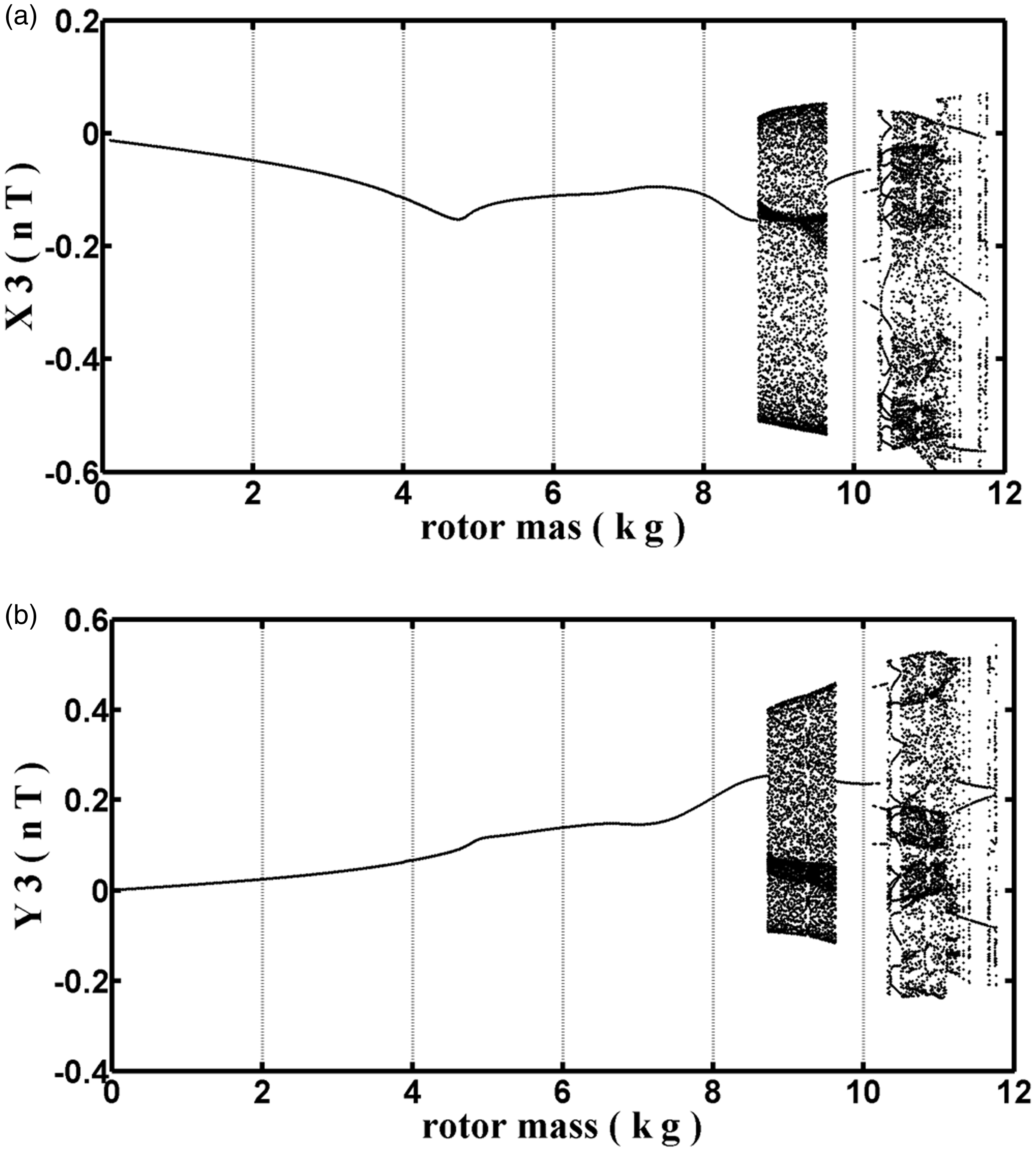
Shown in Figure 5, the rotor mass mr is taken as an analysis parameter to explore the effect of different rotor masses on the system, while setting the mass range from 0.01 to 9.4 kg for the actual operating conditions. From Figures 5 to 7, we can see that system instability will occur earlier when the number of bearings (rotation speed) is larger. Therefore, the paper analyzes the influence of the number of bearings (rotation speed) later. At the same time, as it can be seen from Figure 5 when mr < 6.97 kg, the rotor center of the system shows periodic motion in both the horizontal and vertical directions. This phenomenon of motion can be further proved by the Poincaré section (Figure 8(a)). However, as the mass of this cycle motion increased to mr = 6.98 kg, the rotor center will be replaced by quasi-periodic movement, as shown in Figure 8(b), and this state of motion is maintained within the 6.97≤ mr <7.71 kg range. But as the mass increases to mr =7.71 kg, quasi-periodic motion quickly changes to T-periodic motion, and this state can be further confirmed by Figure 8(c).
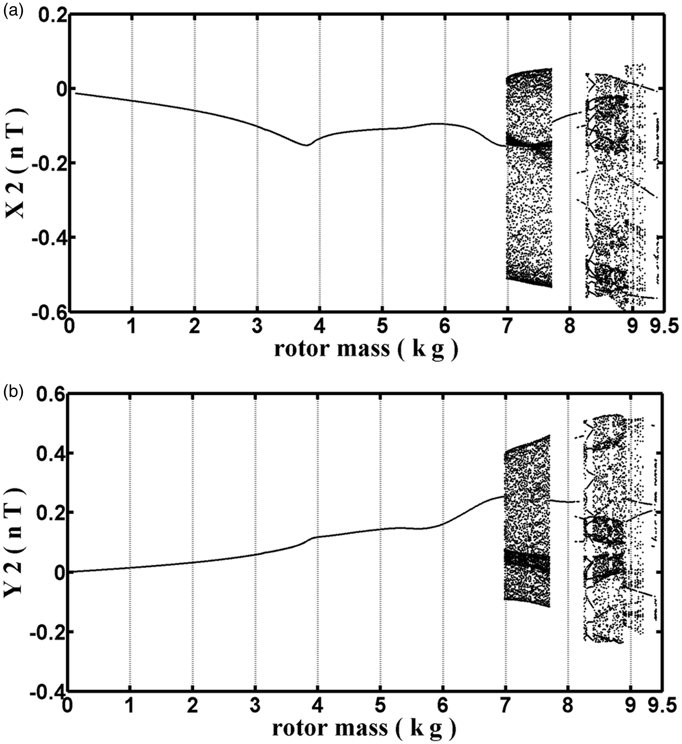
Bifurcation map of the rotor center to different rotor masses: (a) X2(nT); (b) Y2(nT), the number of system bearings Λ = 4.5.
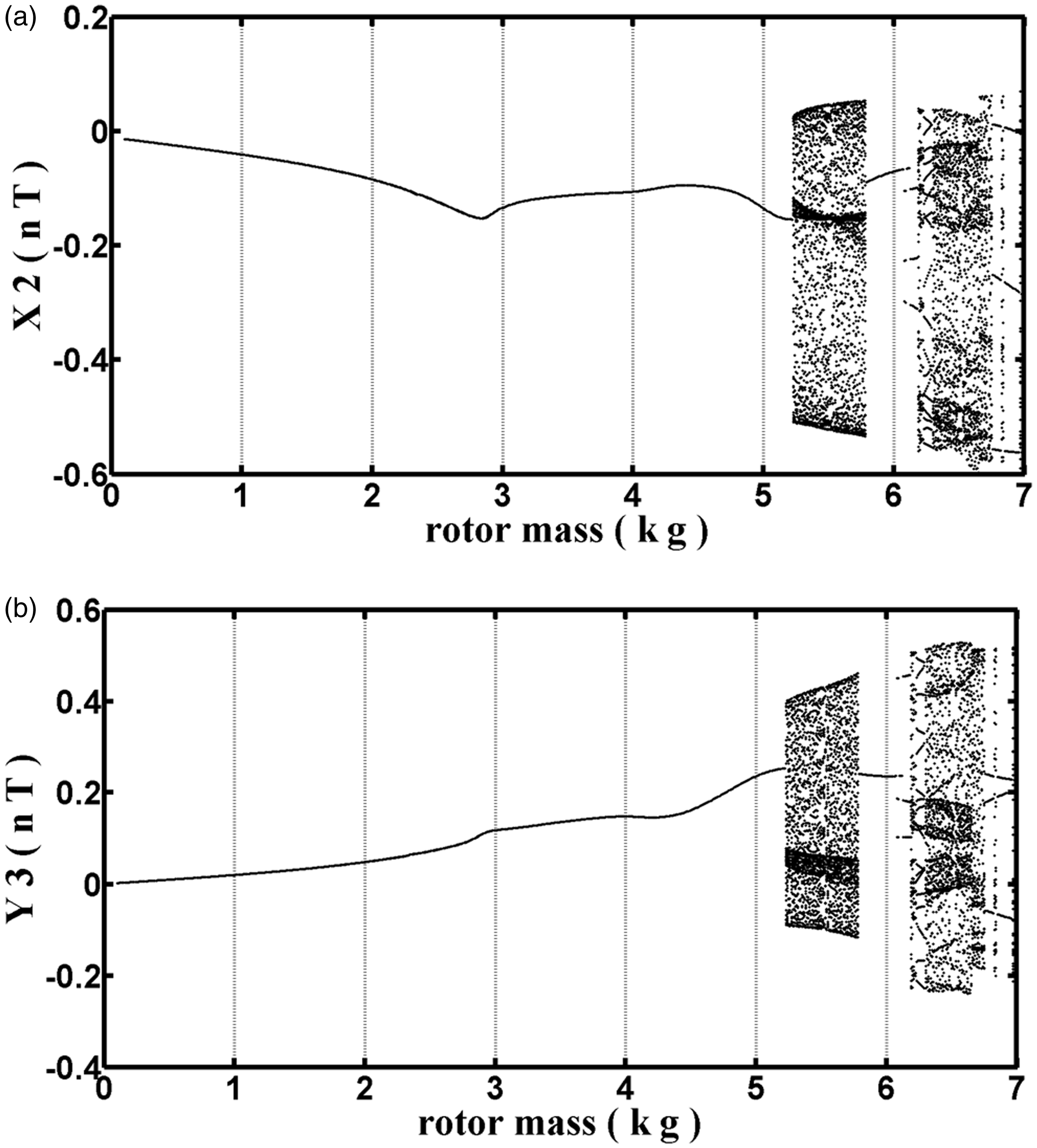
Bifurcation map of the rotor center to different rotor masses: (a) X2(nT); (b) Y2(nT), the number of the system bearing Λ = 6. 0.
Bifurcation map of the rotor center to different rotor masses: (a) X2(nT); (b) Y2(nT), the number of the system bearing Λ = 2.0.
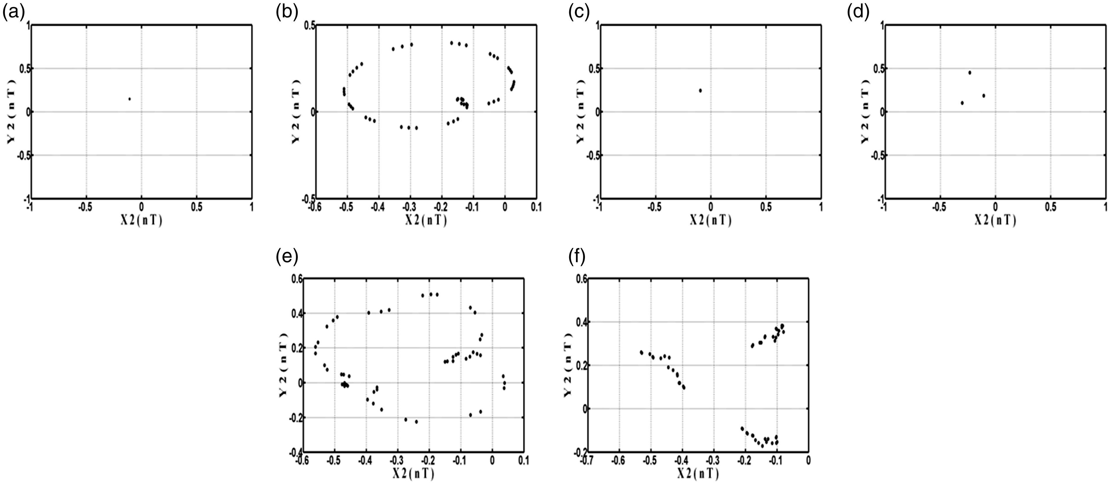
Poincaré sectional view of the rotor center at different rotor masses: (a) mr = 5.3; (b) 6.98; (c) 7.71; (d) 8.11; (e) 8.25; (f) 9.39 kg (system bearing number Λ = 4.5).
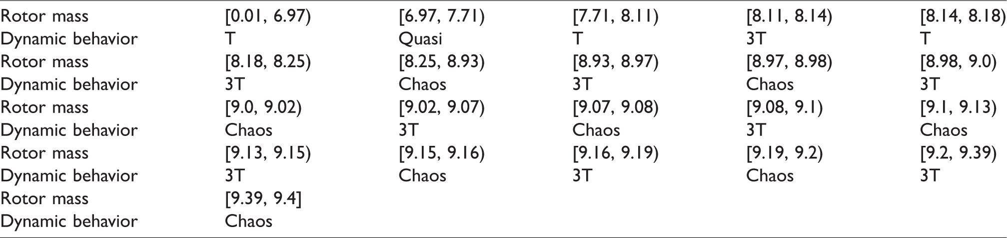
When the mass increases to mr =8.11 kg, the system turns to the sub-cycle motion, as shown in Figure 8(d), while the movement is only maintained at 8.11≤ mr <8.14kg range. As the mass continues to increase to mr =8.18 kg, the system’s motion behavior is T and 3T intermittent movement. This phenomenon occurs in the 7.71≤ mr <8.25kg range. When mr =8.25kg, the system turns from 3T cycle to chaotic movement. The movement is only maintained at 8.25≤ mr <8.93kg. Afterward the system presents the movement of Chaos and 3T vibration forms. The movement is only maintained at 8.25≤ mr ≤9.4 kg range. When mr =8.25 and 9.39 kg, the system is in a state of chaotic motion, which can be further proved by Figures 8(e) and (f). From the above results showing that the rotor movement patterns also showed a considerable degree of cyclical order, the following are the movement patterns presented by the system for rotors with different masses and makes a whole summary as shown in Table 5.
Rotor center dynamic behavior under the rotor mass change (system bearing number Λ = 4.5).
Shown by Figure 8(a), (c) and (d), while mr =5.3, 7.71, 8.11 kg, the motion of the bearing presented in a Poincaré sectional view is a single point or three discrete points, the system is in a single cycle movement or 3T periodic motion. If the motion state shown in Figure 8(b) is a single closed curve formed by multiple discrete points, it shows quasi-periodic motion, while Figure 8(e) and Figure 8(f) are irregular discrete points, which means the system is in chaotic movement.
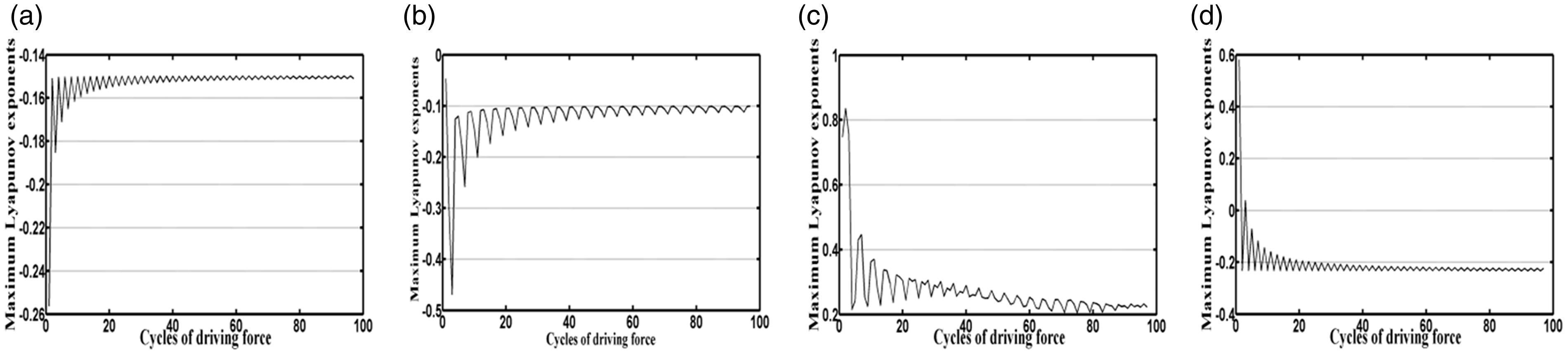
For the confirmation of chaos behavior, in the execution of this paper, interpret and further verify the maximum Lyapunov exponents. As it can be seen from Figure 9(a) to (d), as mr = 5.3, 6.98, 7.71, 8.11 kg, and the Lyapunov index tends to zero, then the system is nonchaotic behavior. And when mr =8.25 and 9.39, as shown in Figure 9(e) and (f), the index is greater than zero, so the system’s motion state is indeed chaotic behavior. At the same time, the overall Lyapunov exponent for the system is also shown in Figure 10, which shows that the region of chaos (index greater than zero) occurs in several intervals, especially within the 8.25≤ mr ≤9.4 kg range, which is consistent with the results summarized in Table 5.
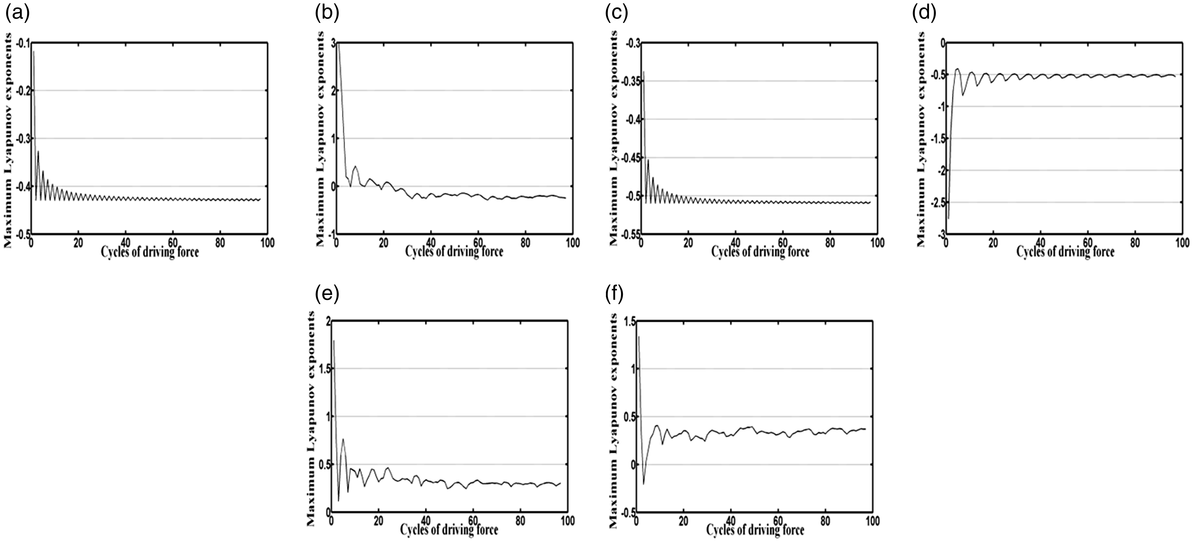
Lyapunov index of the rotor center at different rotor masses: (a) mr = 5.3; (b) 6.98; (c) 7.71; (d) 8.11; (e) 8.25; (f) 9.39 kg (system bearing number Λ = 4.5).
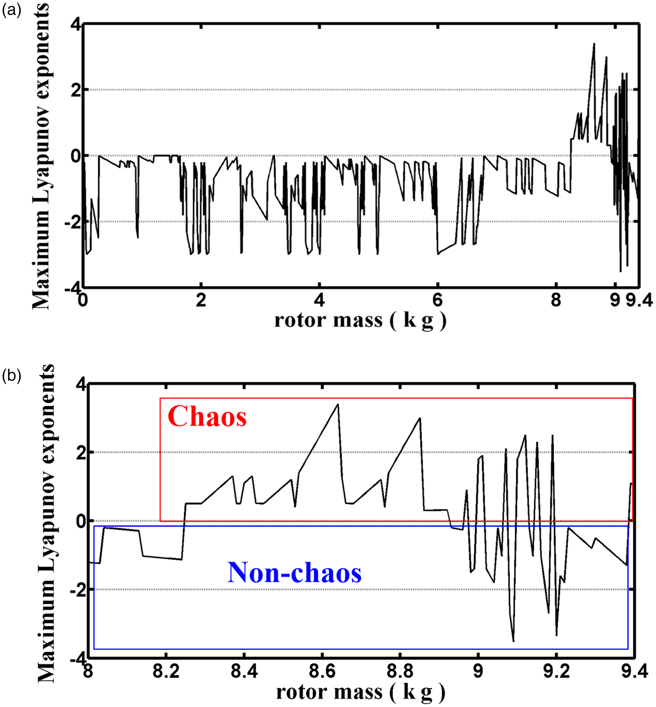
Maximum Lyapunov exponent with different rotor masses: (a) overall; (b) 8.0 ≤ mr ≤ 9.4 kg (system bearings number Λ = 4.5).
Effect of the bearing number Λ on the system
Take an obverse wedge shape opposing bearing as an example. The rotor speed will affect the related performance of the entire system, and therefore the bearing number Λ is taken as a bifurcation parameter, the rotor mass is set as mr =3.5 kg, and analyze the dynamic system behavior.
Dynamic trajectory map
From Figure 11.1(a), (b), 11.2(a), (b),…, 11.4(a), (b) it can be observed that, when there is a small number of bearings (Λ = 3.2), the behavior presented by the rotor is more regular, and when Λ increases to 5.07, the system still shows regular motion. When the bearing number reaches 6.51, the dynamic trajectory changes to non-regular motion, and when Λ = 6.97, the behavior of the rotor center is transformed into a regular phenomenon.
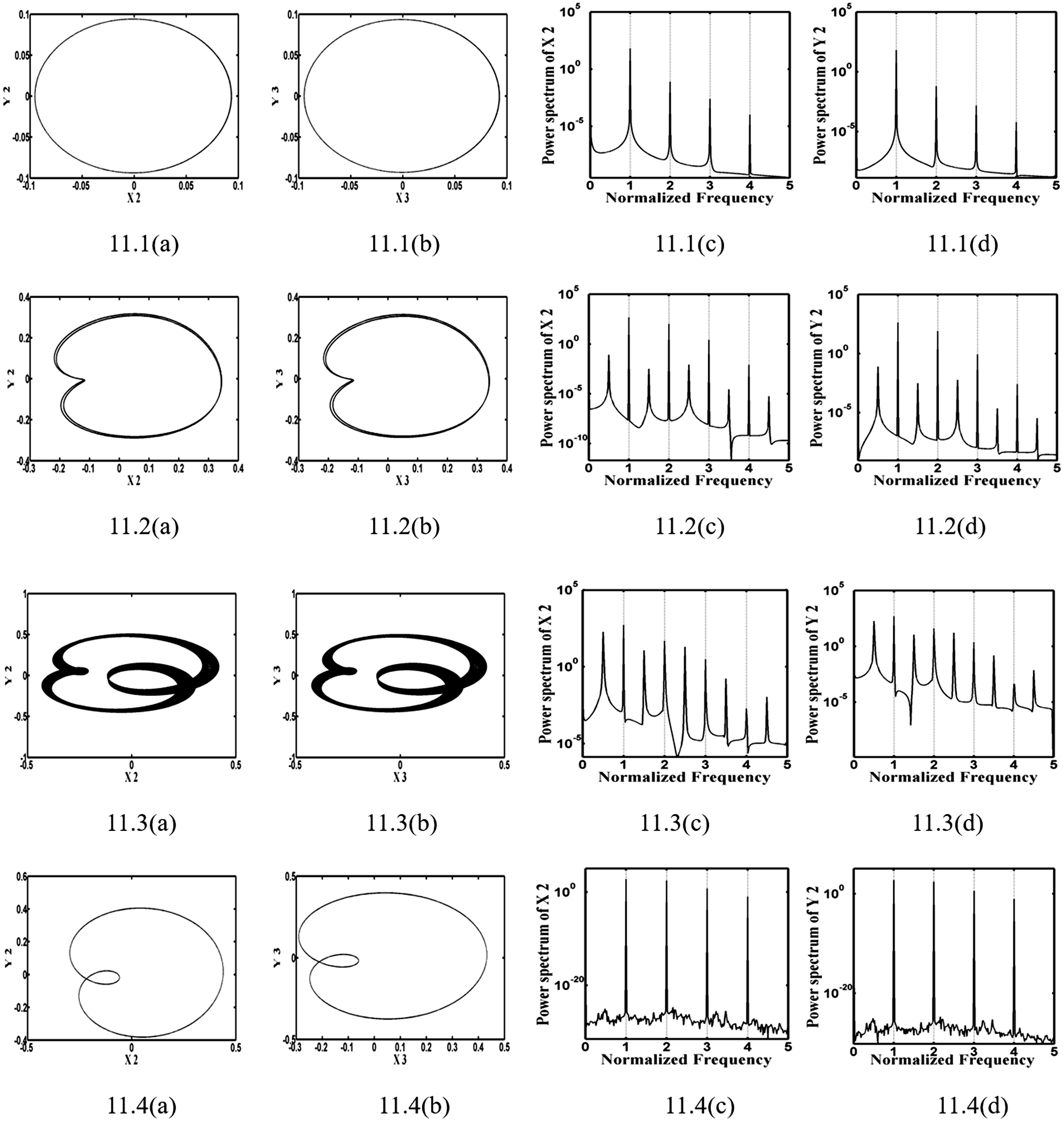
Rotor center dynamic trajectory (Figure 11.1(a) to 11.4(a)) when the bearing number is Λ = 3.2, 5.07, 6.51, 6.97, journal center dynamic trajectory map (Figure 11.1(b) to 11.4(b)), spectral response of the center of the rotor in the horizontal direction (Figure 11.1(c) to 11.4(c)) and the vertical direction (Fig 11.1(d) to 11.4(d)) (rotor mass as mr=3.5 kg).
b. Spectrum analysis map
Figure 11.1(c), (d), 11.2(c), (d),…, 11.4(c), (d) display the dynamic response of the rotor center in horizontal and vertical directions with a different number of bearings. Research shows when the number of bearings is Λ = 3.2, the rotor center presents T-periodic motion, and when Λ = 5.07, the spectral response graph (Figure 11.2(c), (d)) displays the rotor center presenting 2T subharmonic motion both in the horizontal and vertical directions. As the number of bearings increases to Λ = 6.51, the mode of motion transforms into nonlinear chaotic motion. At Λ = 6.97, the system turns into T-periodic motions, and its shape is the same both in the horizontal and vertical directions.
c. Bifurcation diagram
As shown in Figure 12, the number of bearings Λ is taken as the main analysis parameter, to study the effect of the bearing number Λ on systems, while setting the range of the number of bearings from 1.0 to 7.5 for the actual operating conditions. When the number of low bearings is Λ = 3.2, regardless of the horizontal and vertical directions, the system rotor center presents T-period movement, this phenomenon may be verified by Figure 13(a). When increasing the number of bearings to Λ = 5.07, the system in turn generates 2T movement, and from Figure 13(b) it is clear at this time that the system generates two discrete points. This 2T movement stands at just 5.07≤Λ < 6.51. When increasing the number of bearings to Λ = 6.51, the system turns to produce chaotic motion, this status may be further verified by Figure 13(c) and this motion state is maintained within the range 6.51 ≤ Λ < 6.97. As Λ increases to 6.97, the bearing system tends to be stable and exhibits T-period motions, as shown in Figure 13(d).
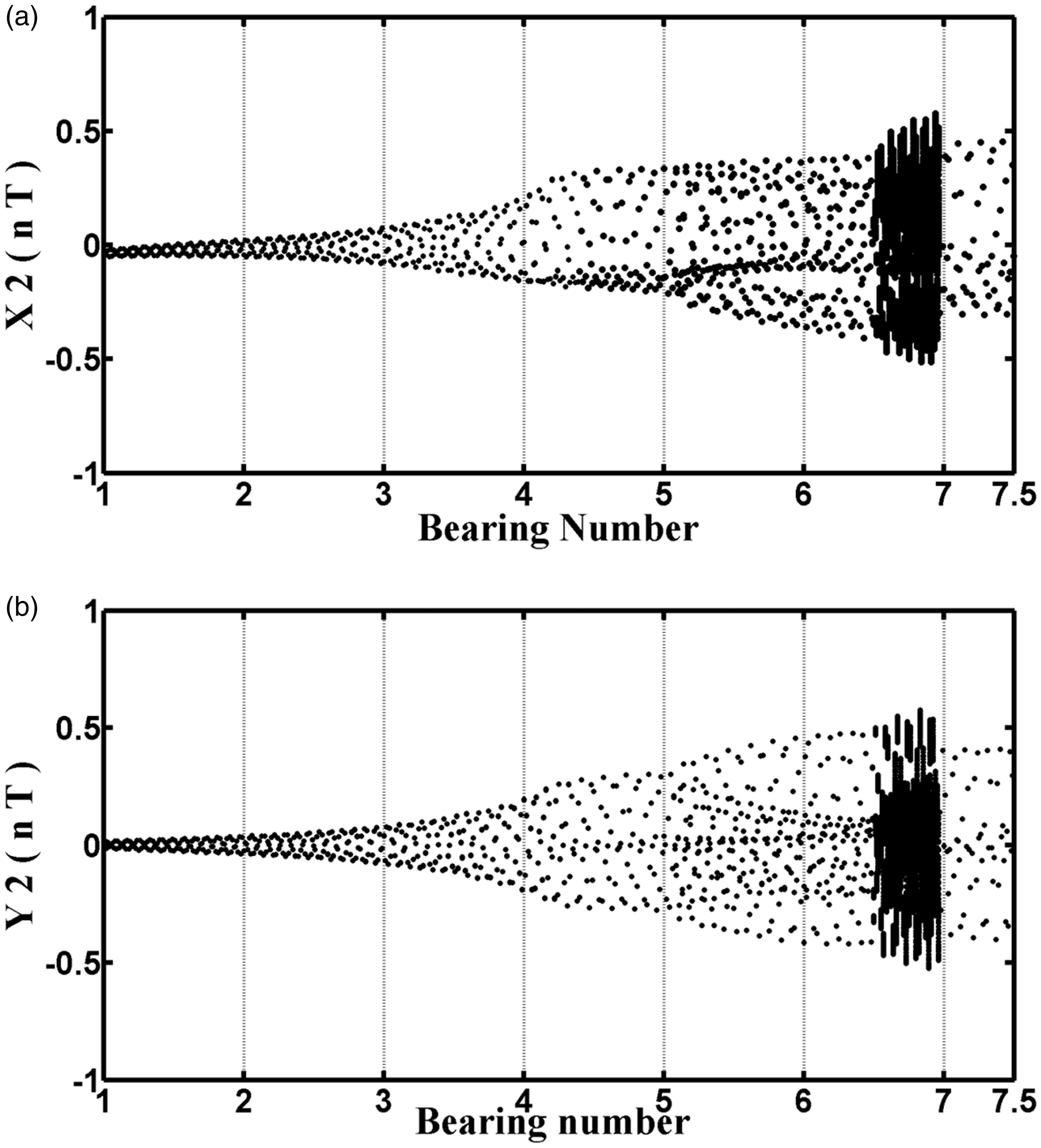
The bifurcation diagram of the rotor center for different bearing numbers Λ: (a) X2(nT); (b) Y2(nT) (rotor mass at mr=3.5 kg).
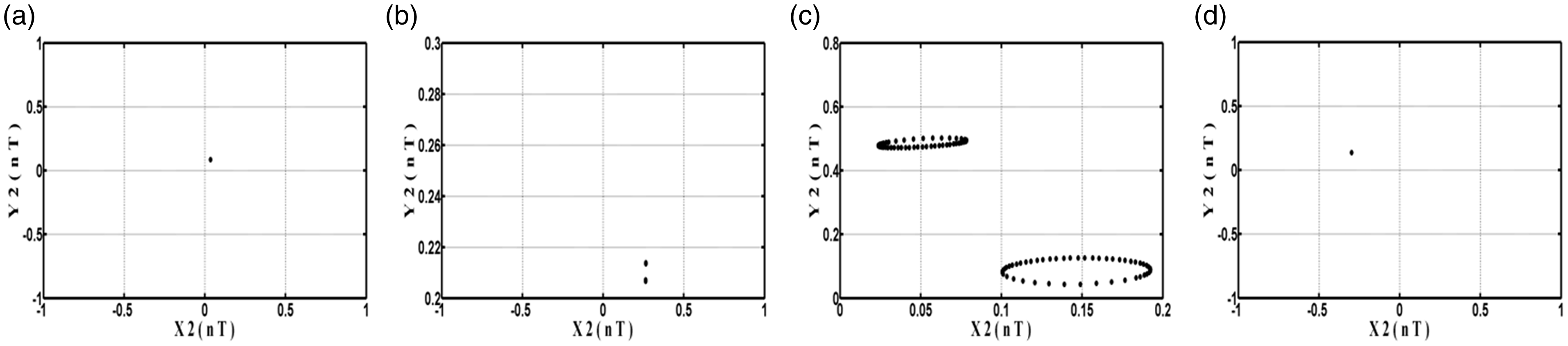
Poincaré cross-sectional view of the center of the rotor in different number of bearing: (a) Λ = 3.2; (b) 5.07; (c) 6.51; (d) 6.97 (rotor mass at mr=3.5 kg).
The relationship between the rotor center motion and the number of bearings is quite complex, so the range of 1.0 ≤ Λ ≤ 7.5 is summarized in Table 6 as follows.
Dynamic behavior of the rotor center with different bearing numbers (1.0 ≤ Λ ≤ 7.5, the rotor mass as mr=3.5 kg).

For the confirmation of chaos behavior, in the execution of this paper, we further verify and interpret the maximum Lyapunov exponents. From Figure 14(a), (b), and (d) it can be seen that when Λ = 3.2, 5.07, 6.97, and the Lyapunov exponents are less than zero, the system is in nonchaotic behavior. When Λ = 6.51, in Figure 14(c), the index is greater than zero, so the system motion state is indeed chaotic behavior. While the whole picture of the influence of the system’s Lyapunov exponents on the changing bearings number is also shown in Figure 15, the results show a chaotic region (index greater than zero) occurs only in the 6.51≤Λ < 6.97 range, and the remaining area is a stable operating range, which is consistent with the results summarized in Table 6.
Lyapunov exponents of rotor center behavior at bearing number: (a) Λ = 3.2; (b) 5.07; (c) 6.51; (d) 6.97 (rotor mass at mr=3.5 kg).
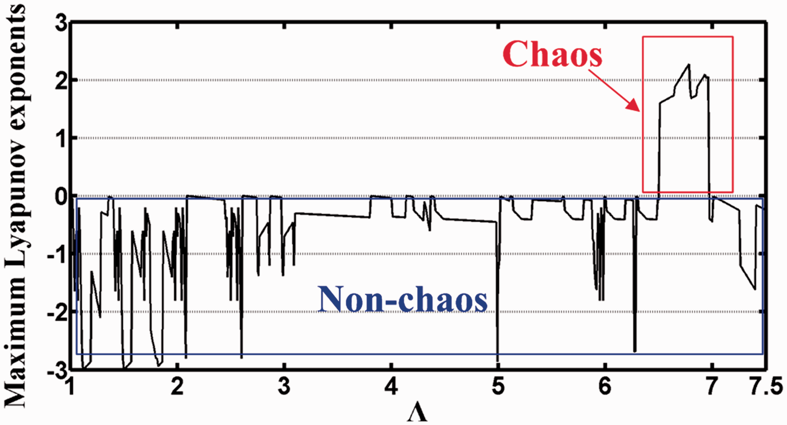
Overall system Lyapunov exponent with different bearing numbers (rotor mass at mr = 3.5 kg).
Stable and unstable areas for OHGB system considering various rotor masses and bearing numbers
In order to know whether the behavior of the bearing system under various parameters is stable or not, this paper uses different rotor masses and bearing numbers as the analysis parameters and constructs both stable and unstable regions of the shaft through Lyapunov exponents, as shown in Figure 16. The white, red, and pink blocks in the figure belong to the unstable region while the other color blocks belong to the stable region. Therefore, the unstable regions of the system are mostly concentrated in the upper right corner of the figure (the rotor mass and bearing number are larger). And in the low number of bearings, the system is stable and has periodic motion, the results can effectively identify and establish the stable and unstable areas of the opposed-type high-speed gas bearing system in operation, and can be used as an important reference basis for the follow-up bearing system design.
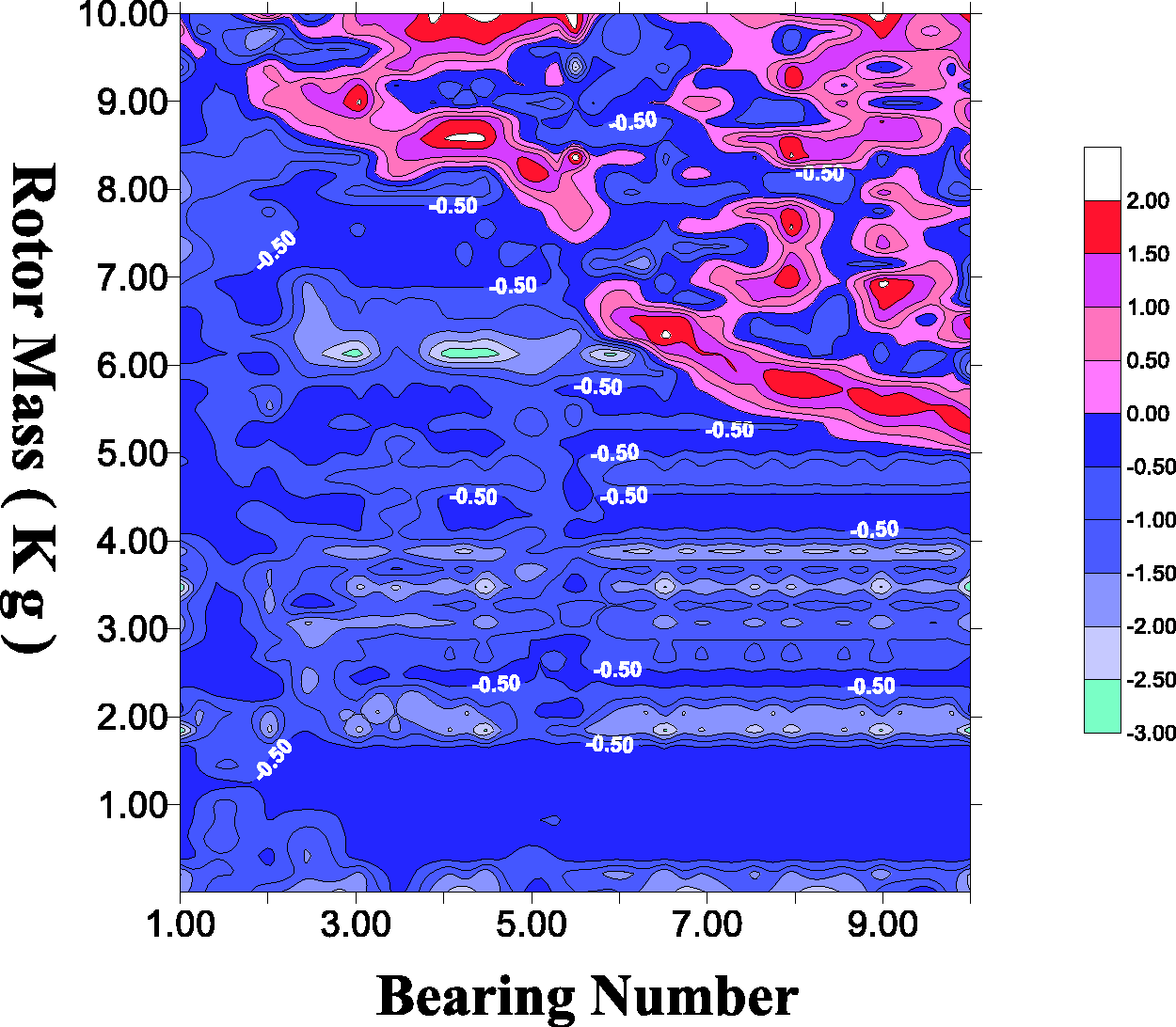
Full-size image of Lyapunov exponents of stable and unstable areas of opposed high-speed gas bearing systems.
Conclusion
The objective of this study was an analysis of the dynamic behavior of a flexible rotor supported by an OHGB system. The FDM, perturbation method, and a mixing method were used to solve the pressure distribution at the highest nonlinearity in the system, after which dynamic equations of the flexible rotor center were used to obtain the orbits of the rotor center. Analysis was then conducted on the orbit data to generate spectrum diagrams, Poincaré maps, bifurcation diagrams, and maximum Lyapunov exponents. This showed that the orbits of the rotor center change along with the mass and the bearing number and synchronously generate complicated motion in the horizontal and vertical directions, include normal and sub-harmonic vibration, as well as periodic, quasi-periodic, and chaotic motion. The mixing method applied in this paper yields better accuracy and precision for the verification of values than the FDM and perturbation method. Accurate solutions can be obtained without the need for very precise position and time step determination. Findings with respect to the motion and behavior of the rotor revealed that the rotor orbits demonstrate unstable nonlinear chaotic behavior when the mass of the rotor is high but the system is relatively stable at the other intervals and ranges. The bearing number affects the orbits of the rotor, which show chaotic behavior in the interval 3.84 ≤ Λ < 3.86 while the orbits in the other intervals and ranges show relatively organized and stable motion. The results obtained in this study can be used as a basis for future OHGB system design and the prevention of instability.
Footnotes
Declaration of conflicting interests
The author(s) declared no potential conflicts of interest with respect to the research, authorship, and/or publication of this article.
Funding
The author(s) disclosed receipt of the following financial support for the research, authorship, and/or publication of this article: This study was funded by the Ministry of Science and Technology of Taiwan (Grant numbers MOST-106–2221-E-167–012-MY2 and MOST-106–2622-E-167–010-CC3).