Effective finite element model in-loop system of laminated cylindrical structure for multiple inputs and multiple outputs active vibration control

Abstract

Active vibration control of large laminated cylindrical structures, for example, the cabin of space, air, surficial or subaqueous vehicles, usually requires multiple inputs and multiple outputs to the system, since there are usually multiple vibration sources and each source contains multiple frequency components. The performance of multiple inputs and multiple outputs control system will be dramatically affected by the complex dynamic behavior of the laminated cylindrical structure, thus an effective model is in great request in analyzing and designing the control system. However, there is seldom distributed parametric model, typically, finite element model, applying to the active vibration control system, because of its computational complexity. In this work, we propose an effective finite element model in-loop system of laminated cylindrical structure for multiple inputs and multiple outputs active vibration control simulation. Firstly, an finite element model of laminated thick cylindrical structure with four-node Mindlin degenerated shell element has been constructed. Then, a model reduction procedure has been proposed to obtain in-loop model of the control system. The numerical global modal analysis and harmonic response analysis of the cylindrical structure have been conducted to verify the correctness of the model. Afterward, a multiple inputs and multiple outputs adaptive algorithm which is able to coup with multiple frequencies and multiple sources vibration has been applied to the finite element model in-loop system. Finally, four numerical case studies have been conducted, in which the vibration sources contain multiple frequency components and artificial colored noises. The result shows that the vibration of the multiple control points can be dramatically suppressed simultaneously, which demonstrates the effectiveness of the algorithm and finite element model in-loop system.

Introduction

In recent years, active vibration control (AVC) has drawn extensive attentions to researchers in field of engineering, since unwelcome noise and vibration need urgently to be suppressed for sake of safety, durability, comfort, or stealth.^1–7 The AVC of large laminated cylindrical structure, for example, the cabin of space, air, surficial or subaqueous vehicles, usually requires multiple inputs and multiple outputs (MIMO) to the system, since there are usually multiple vibration sources and each vibration source contains multiple frequencies components. A model plays extremely important role in MIMO AVC system. They can be used for system analysis, for controller design, for prediction of system dynamic, for stability investigation of system, as an add-in model to system, etc. Although large amount of studies has been devoted to the modeling of AVC system,^8–16 the model embedded into the control loop is mainly lumped parametric model or data-based model rather than distributed parametric model, typically, finite element (FE) model.

FE model is a very important tool to describe complex object whose analytical model is hard or even impossible to obtain. Embedding an FE model into the control loop is tempting since it adds space dimension to the control system and can investigate the global response of the object before and after control. However, FE model is seldom been applied to AVC system, because of its computational complexity. A large FE model will usually take minutes or even hours to calculate the dynamic response. It is intolerable to take a few seconds finishing one control loop, needless to say minutes or even hours.

With the development of computer technology, there are researchers spare no effort to apply FE model to on-line simulation system. Studies on simple structures like beam, plate or shell were reported. Lin et al.¹⁷ proposed an active control with optical fiber sensors and neural networks. Balamurugan and Narayanan¹⁸ proposed a nine-node piezo-laminated degenerated shell FE to model the multilayer composite shell structure for AVC. Xu and Koko¹⁹ studied the AVC of a smart beam, where the FE model is constructed by ANSYS. Kapuria and Yasin^20–22 investigated the AVC of a laminated beam with piezoelectric actuators/sensors and a multilayered plate integrated with piezoelectric fiber reinforced composites, respectively. Khot et al.²³ studied the AVC of a piezoelectric beam using PID algorithm by extracting the state-space (SS) model from the FE model. Karagulle et al.²⁴ integrated the AVC algorithm into the FE model of smart beam using APDL language in ANSYS. Maruani et al.²⁵ conducted a numerical efficiency study on the AVC for an FE model of functionally graded piezoelectric material beam. Lu et al.²⁶ studied the AVC of clamped-clamped thin-plate structures with partial SCLD treatment based on its FE model. Rao et al.²⁷ investigated the finite rotation FE-simulation and AVC of smart composite laminated structures based on four-node shell element. Liu et al.^28,29 studied the coupling system of actuator and structure based on extracting of FE model. Oveisi et al.³⁰ introduced a new framework for running the FE package inside an online loop together with MATLAB.

To improve the computational efficiency of FE model, some of the above-mentioned studies make improvements in the stage of modeling, e.g. using degenerated shell element rather than solid element.^18,31 Some others concentrate on model reduction, e.g. extracting the SS model from FE model by CAE software.^{19–21,23,24,32–34} However, they still do not meet the requirement to embed FE model of large structure into AVC simulation, since the degree of freedoms (DOFs) and order of modes of large FE model are very high. Moreover, once the SS model is extracted, the reduced model is determined and it is not easy to extend the dimensions of in-loop model or investigate the response of nodes that are not extracted.

In this paper, we construct FE model of a complex laminated cylindrical structure and embed it into the AVC control, which is named as finite element model in-loop system (FEMilS). The geometry formulation is presented in detail based on a Mindlin degenerated shell element. An effective preprocessing procedure of FE model is proposed to prepare in-loop model of AVC. An MIMO adaptive algorithm has been applied to FEMilS. The results of numerous case studies verified the effectiveness of the algorithm as well as the FEMilS. This paper is structured as follows. Section ‘Finite element model in-loop system’ gives a detailed description of FEMilS. Section ‘FE modeling of laminated cylindrical structures’ formulates the modeling and preprocessing process of laminated cylindrical structure. Section ‘Numerical implementation’ gives the numerical implementation and visualization of the FE model. Section ‘AVC case study on FEMilS’ conducts the AVC case studies based on FEMilS. Section ‘Conclusion’ concludes the whole paper.

Finite element model in-loop system

Finite element model in-loop system is an effective simulation and verification system for AVC.^35,36 The goal of FEMilS is to design and verify the controller based on the dynamic of the controlled plant. FEMilS is achieved by embedding the FE model of controlled plant, sensors and actuators into the simulation loop of AVC. FEMilS is a time domain point-by-point simulation system whose procedure and structure are extremely similar to that of real-life control. The general procedure of FEMilS is shown in Figure 1. It can be divided into four stages, i.e. geometric modeling, modal analysis, in-loop simulation and postprocessing. In the geometric modeling stage, a simplified model can be first obtained by geometrical simplification and DOFs reduction. Then, the global mass matrix, global stiffness matrix and/or global damping matrix are extracted. In the modal analysis stage, the model can be further reduced by modal reduction and sub-system reduction. Then, the reduced modal mass matrix, reduced modal stiffness matrix, reduced modal damping matrix and reduced eigenmatrix are obtained. In the in-loop simulation stage, an in-loop model for simulation is first constructed according to the above-reduced matrixes. Then, the dynamic response analysis and AVC are conducted. In the post-processing stage, the response reconstruction and comprehensive result demonstration can be conducted. The first two stages can be viewed as pre-processing which prepares the in-loop model for simulation. The third stage is the finally simulation stage.

Figure 1.

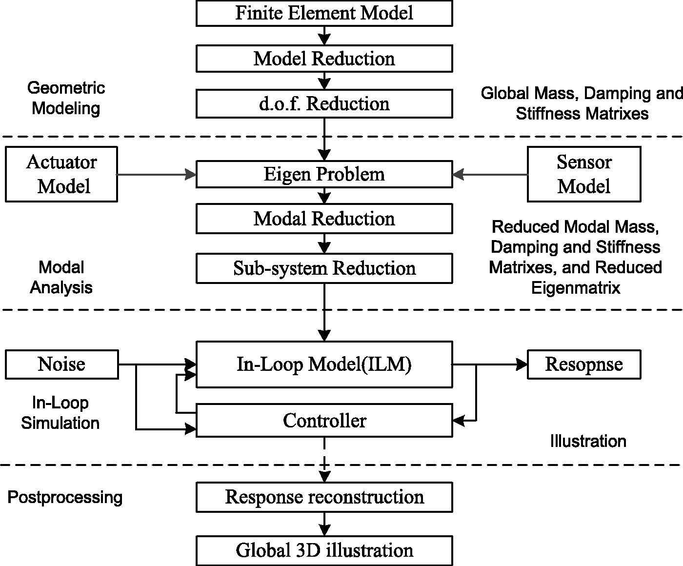
Procedure of FEMilS.

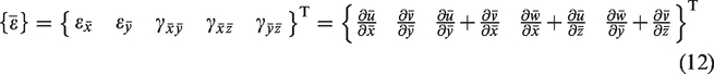
FE modeling of laminated cylindrical structures

Laminated cylindrical structures are widely used in fields of aeronautics and astronautics, vehicle, underwater vehicle, etc. The cylindrical structure can be modeled and analyzed by FE method. The basic FE element for the cylindrical structure modeling is shell element. There are generally two categories of shell elements: one is shell as an assembly of flat elements, and the other one is shell as special case of three-dimensional element. The first one neglects the transverse shear deformation and can only apply for thin shell. The later one considers the transverse shear deformation and can solve thick shell problem as well as laminated shell problem. For a shell element, the thickness dimension is considerably smaller than the other two dimensions. Even for a very thick shell, three or more nodes along thickness-direction supply more DOFs than needed. We eliminate the middle nodes and assume that the adjacent thickness-direction nodes have the same thickness-direction displacement. So, there are five DOFs related to each pair of thickness-direction nodes and they can be attached to a single node whose DOFs are three translations and two rotations.

Geometry of a degenerated shell element

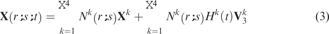
Consider a degenerated four nodes shell element obtained by degenerating the eight nodes solid brick element as shown in Figure 2. It is a Mindlin-type element and is able to coup with transverse shear deformation.

Figure 2.

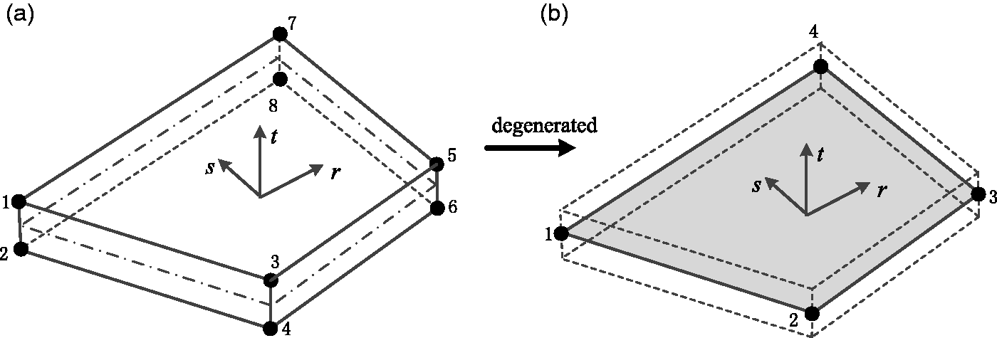
Four nodes shell element degenerated from eight nodes solid element (a) eight nodes solid brick element; (b) four nodes shell element.

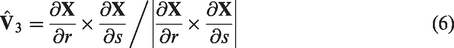
The coordinate systems of degenerated four-node element are shown in Figure 3. The degenerated element is defined by three coordinate systems: the natural coordinate system $\left(r,s,t\right)$ (also called curvilinear coordinate system), the global Cartesian coordinate system $\left(x,y,z\right)$ and the local Cartesian coordinate system $\left(\overline{x},\overline{y},\overline{z}\right)$ . To define the node displacements and an arbitrary local Cartesian coordinate system, orthonormal basis, i.e. $\left({\widehat{\mathbf{V}}}_1^k,{\widehat{\mathbf{V}}}_2^k,{\widehat{\mathbf{V}}}_3^k\right)$ and $\left({\hspace{0.17em}}_{\widehat{\mathbf{V}}}^1,{\hspace{0.17em}}_{\widehat{\mathbf{V}}}^2,{\hspace{0.17em}}_{\widehat{\mathbf{V}}}^3\right)$ , are also defined. The shape functions to describe the mid-surface in terms of r-s plane of natural coordinates are

$$N^k\left(r,s\right)=\frac{1}{4}\left(1+r_{k}r\right)\left(1+s_{k}s\right)\hspace{1em}\left(k=1,2,3,4\right)$$

(1)

where $r_k$ and $s_k$ are the coordinates of the node $k$ in natural coordinates system. The shape functions perpendicular to the mid-surface are

$$H^k\left(t\right)=\frac{1}{2}{\eta }_{k}t\hspace{1em}\left(k=1,2,3,4\right)$$

(2)

where ${\eta }_k$ is the thickness of the shell at the node $k$ . If we assume the thickness of the shell element to be constant, then ${\eta }_k\equiv \eta$ . After the shape functions are defined, the Cartesian coordinates of arbitrary point in the shell can be uniquely given in terms of nodal coordinates and thickness as

$$\mathbf{X}\left(r,s,t\right)={\displaystyle \sum _{k=1}^4{N}^k\left(r,s\right){\mathbf{X}}^k}+{\displaystyle \sum _{k=1}^4{N}^k\left(r,s\right)H^k\left(t\right){\mathbf{V}}_3^k}$$

(3)

where $\mathbf{X}\left(r,s,t\right)={\left\{\begin{array}{ccc}x& y& z\end{array}\right\}}^{\text{T}}$ denotes the global Cartesian coordinates of an interest point, ${\mathbf{X}}^k={\left\{\begin{array}{ccc}{x}^k& y^k& z^k\end{array}\right\}}^{\text{T}}$ denotes global coordinates of node $k$ and ${\widehat{\mathbf{V}}}_3^k={\left\{\begin{array}{ccc}{V}_{31}^k& V_{32}^k& V_{33}^k\end{array}\right\}}^{\text{T}}$ denotes a unit vector perpendicular to the mid-surface. As the strain in the direction perpendicular to the mid-surface will be assumed to be negligible, the displacement throughout the element will be taken to be uniquely defined by the three Cartesian components of the mid-surface nodal displacement $k$ and two nodal rotations ${\alpha }^k$ and ${\beta }^k$ about two unit nodal vectors ${\widehat{\mathbf{V}}}_2^k={\left\{\begin{array}{ccc}{V}_{21}^k& V_{22}^k& V_{23}^k\end{array}\right\}}^{\text{T}}$ and ${\widehat{\mathbf{V}}}_1^k={\left\{\begin{array}{ccc}{V}_{11}^k& V_{12}^k& V_{13}^k\end{array}\right\}}^{\text{T}}$ . The two vectors are perpendicular to each other and to ${\widehat{\mathbf{V}}}_3^k$ . So displacements of an arbitrary point in the element are

$$\mathbf{U}\left(r,s,t\right)={\displaystyle \sum _{k=1}^4{N}^k\left(r,s\right){\mathbf{U}}^k}+{\displaystyle \sum _{k=1}^4{N}^k\left(r,s\right)H^k\left(t\right)\left(-{\mathbf{V}}_2^k{\hspace{0.17em}}_{\overline{\alpha }}^k+{\mathbf{V}}_1^k{\overline{\beta }}^k\right)}$$

(4)

where $\mathbf{U}\left(r,s,t\right)={\left\{\begin{array}{ccc}u& v& w\end{array}\right\}}^{\text{T}}$ denotes the displacement in the direction of global axes. ${\mathbf{U}}^k={\left\{\begin{array}{ccc}{u}^k& v^k& w^k\end{array}\right\}}^{\text{T}}$ denotes the mid-surface nodal displacement along global axis.

Figure 3.

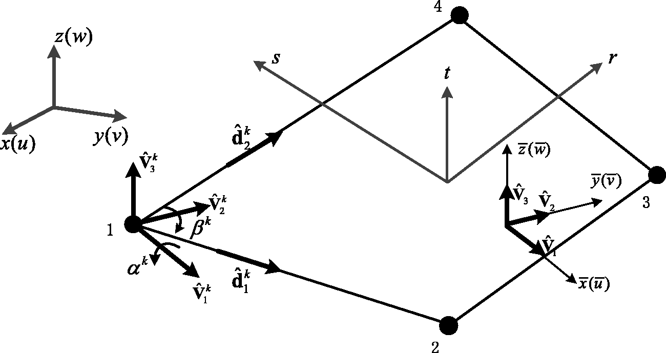
Coordinate systems of the degenerated shell element.

To define the orthonormal basis $\left({\widehat{\mathbf{V}}}_1^k,{\widehat{\mathbf{V}}}_2^k,{\widehat{\mathbf{V}}}_3^k\right)$ , two unit vectors ${\widehat{\mathbf{d}}}_1^k$ and ${\widehat{\mathbf{d}}}_2^k$ start from node $k$ and point to the nodes next to $k$ that are defined first. Thus, the unit normal vector at node $k$ is ${\widehat{\mathbf{V}}}_3^k={\widehat{\mathbf{d}}}_1^k\times {\widehat{\mathbf{d}}}_2^k$ . As an infinity vector directions that normal to ${\widehat{\mathbf{V}}}_3^k$ can be generated, we defined ${\widehat{\mathbf{V}}}_1^k,{\widehat{\mathbf{V}}}_2^k$ as follows to make them unique:

$${\widehat{\mathbf{V}}}_1^k=\mathbf{j}\times {\widehat{\mathbf{V}}}_3^k,{\widehat{\mathbf{V}}}_2^k={\widehat{\mathbf{V}}}_3^k\times {\widehat{\mathbf{V}}}_1^k$$

(5)

where $\mathbf{j}$ is the unit vector along y axis. If $\mathbf{j}$ and ${\widehat{\mathbf{V}}}_3^k$ are occasionally in the same direction, we let ${\widehat{\mathbf{V}}}_3^k=\left(1,0,0\right)$ to avoid the invalidation of equation (5).

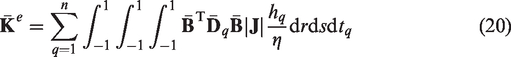
In fact, the rotations at node $k$ are shared by all the elements that share node $k$ . To ensure that the z-axis is perpendicular to the mid-surface at node $k$ , it is possible that the set of $\left({\alpha }^k,{\beta }^k,{\gamma }^k\right)$ directions will differ from node to node. The strain–displacement can be derived under an arbitrary local Cartesian coordinate system of the element. For an arbitrary point in the mid-surface, we erect a normal $\overline{z}$ with two other orthogonal axes $\overline{x}$ and $\overline{y}$ tangent to it. Assume ${\widehat{\mathbf{V}}}_3$ is a unit normal vector in the mid-surface to decide the direction of $\overline{z}$ , it is defined (from equation (3)) as

$${\widehat{\mathbf{V}}}_3=\frac{\partial \mathbf{X}}{\partial r}\times \frac{\partial \mathbf{X}}{\partial s}/\left|\frac{\partial \mathbf{X}}{\partial r}\times \frac{\partial \mathbf{X}}{\partial s}\right|$$

(6)

Following the process which defines uniquely two perpendicular vectors before in equation (5), we construct unit vector ${\widehat{\mathbf{V}}}_1$ and ${\widehat{\mathbf{V}}}_2$ in $\overline{x}$ and $\overline{y}$ direction, respectively. By assembling them together, we got a direction cosine matrix

$$\Theta ={\left\{\begin{array}{ccc}{\widehat{\mathbf{V}}}_1& {\widehat{\mathbf{V}}}_2& {\widehat{\mathbf{V}}}_3\end{array}\right\}}^{\text{T}}$$

(7)

where $\Theta$ connects the global Cartesian coordinate system to local coordinate system by

$$\mathbf{X}=\Theta \overline{\mathbf{X}}$$

(8)

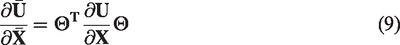
The global derivatives of displacements are now transformed to the local derivatives of the local orthogonal displacements by a standard operation as

$$\frac{\partial \overline{\mathbf{U}}}{\partial \overline{\mathbf{X}}}={\Theta }^{\mathbf{T}}\frac{\partial \mathbf{U}}{\partial \mathbf{X}}\Theta$$

(9)

where $\overline{\mathbf{U}}\left(r,s,t\right)={\left\{\begin{array}{ccc}\overline{u}& \overline{v}& \overline{w}\end{array}\right\}}^{\text{T}}$ denotes the displacements in the direction of local axes; $\overline{\mathbf{X}}={\left\{\begin{array}{ccc}\overline{x}& \overline{y}& \overline{z}\end{array}\right\}}^{\text{T}}$ denotes the local coordinate of an interest point. The derivatives of displacements with respect to the global coordinates are given by

$$\frac{\partial \mathbf{U}}{\partial \mathbf{X}}={\mathbf{J}}^{-1}\frac{\partial \mathbf{U}}{\partial \mathbf{R}}$$

(10)

where J denotes a Jacobian matrix, $\mathbf{R}={\left\{\begin{array}{ccc}r& s& t\end{array}\right\}}^{\text{T}}$ denotes curvilinear coordinate of an interest point. $\frac{\partial \mathbf{U}}{\partial \mathbf{R}}$ is calculated from the displacement definition of equation (4) and the Jacobian matrix J is defined as

$$\mathbf{J}=\frac{\partial \mathbf{X}}{\partial \mathbf{R}}$$

(11)

which is calculated from the coordinate definition of equation (3).

In the local coordinate system, if the basic shell assumptions have been taken into account, the strain vector of interest is

$$\left\{\overline{\epsilon }\right\}={\left\{\begin{array}{l}{\epsilon }_{\overline{x}}{\epsilon }_{\overline{y}}{\gamma }_{\overline{x}\overline{y}}{\gamma }_{\overline{x}\overline{z}}{\gamma }_{\overline{y}\overline{z}}\hfill \end{array}\right\}}^{\text{T}}={\left\{\begin{array}{ccccc}\frac{\partial \overline{u}}{\partial \overline{x}}& \frac{\partial \overline{v}}{\partial \overline{y}}& \frac{\partial \overline{u}}{\partial \overline{y}}+\frac{\partial \overline{v}}{\partial \overline{x}}& \frac{\partial \overline{w}}{\partial \overline{x}}+\frac{\partial \overline{u}}{\partial \overline{z}}& \frac{\partial \overline{w}}{\partial \overline{y}}+\frac{\partial \overline{v}}{\partial \overline{z}}\end{array}\right\}}^{\text{T}}$$

(12)

and the components of strain matrix can be picked from $\frac{\partial \overline{\mathbf{U}}}{\partial \overline{\mathbf{X}}}$ decided by equation (9). Now, the components of the strain-displacement matrix $\overline{\mathbf{B}}$ can be found explicitly

$$\begin{array}{l}\overline{\epsilon }={\overline{\mathbf{B}}}^{\text{T}}{\tilde{\mathbf{U}}}^e={\displaystyle \sum _{k=1}^4{\overline{\mathbf{B}}}_k{\tilde{\mathbf{U}}}_k^e}\\ \overline{\mathbf{B}}={\left[\begin{array}{cccc}{\overline{\mathbf{B}}}_1& {\overline{\mathbf{B}}}_2& {\overline{\mathbf{B}}}_3& {\overline{\mathbf{B}}}_4\end{array}\right]}^{\text{T}}\\ {\tilde{\mathbf{U}}}^e={\left\{\begin{array}{cccc}{\tilde{\mathbf{U}}}_1^e& {\tilde{\mathbf{U}}}_2^e& {\tilde{\mathbf{U}}}_3^e& {\tilde{\mathbf{U}}}_4^e\end{array}\right\}}^{\text{T}}\end{array}$$

(13)

where ${\overline{\mathbf{B}}}_k$ is a sub-matrix relating the strains defined under an arbitrary local coordinate $\left(\overline{x},\overline{y},\overline{z}\right)$ to displacements defined under global coordinate and local coordinate at node $k$ , ${\tilde{\mathbf{U}}}^e$ is the displacement vector of eth element and ${\tilde{\mathbf{U}}}_k^e={\left\{\begin{array}{l}{u}^k{v}^k{w}^k{\overline{\alpha }}^k{\overline{\beta }}^k{\overline{\gamma }}^k\hfill \end{array}\right\}}^{\text{T}}$ is the displacement representation of node $k$ . It is noteworthy that ${\overline{\gamma }}^k$ which denotes the rotation about normal at node $k$ is useless in the local coordinates system. We add it here to make the transformation from local to global coordinates system to be easier. In fact, ${\tilde{\mathbf{U}}}_k^e$ is a ‘mix’ displacement vector, in which $u^k,v^k,w^k$ are defined in the global coordinate system and ${\overline{\alpha }}^k,{\overline{\beta }}^k,{\overline{\gamma }}^k$ are defined in the local coordinate system at node $k$ .

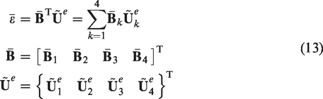
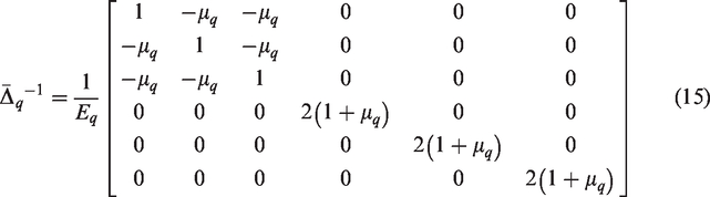
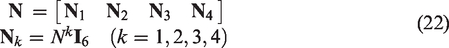
Stiffness matrix of a laminated structure

Most structure of vehicle and underwater vehicle can be view as laminated structure (including the steel layer). Assume $n-1$ layers anechoic materials are added outside the cylindrical steel structure, we got an n layer laminated structure as shown in Figure 4, which is investigated under the same local coordinate system in Section ‘Geometry of a degenerated shell element’.

Figure 4.

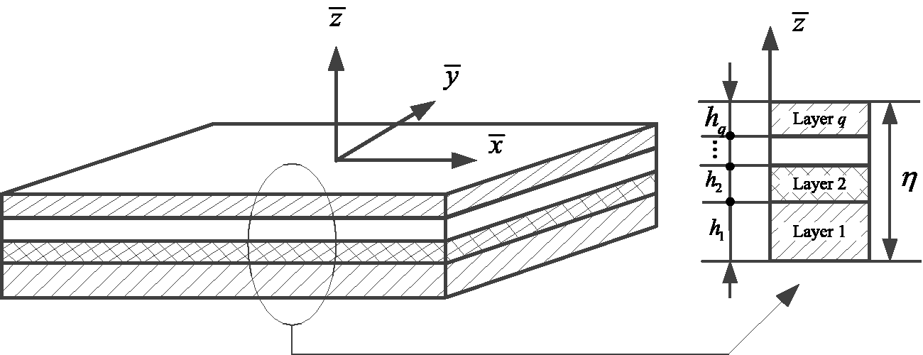
The laminated structure.

For simplicity purpose, assume each layer is isotropic material. So according to Hook’s low, the relationship between stress and strain of layer q is

$${\overline{\sigma }}_q={\overline{\Delta }}_q{\overline{\epsilon }}_q$$

(14)

where ${\overline{\Delta }}_q$ is the elasticity matrix of layer q and ${\overline{\Delta }}_q{\hspace{0.17em}}^{-1}$ is the flexibility matrix and is given by

$${\overline{\Delta }}_q{\hspace{0.17em}}^{-1}=\frac{1}{E_q}\left[\begin{array}{cccccc}1& -{\mu }_q& -{\mu }_q& 0& 0& 0\\ -{\mu }_q& 1& -{\mu }_q& 0& 0& 0\\ -{\mu }_q& -{\mu }_q& 1& 0& 0& 0\\ 0& 0& 0& 2\left(1+{\mu }_q\right)& 0& 0\\ 0& 0& 0& 0& 2\left(1+{\mu }_q\right)& 0\\ 0& 0& 0& 0& 0& 2\left(1+{\mu }_q\right)\end{array}\right]$$

(15)

where E_q is the modulus of layer q and μ_q is Poisson’s ratio of layer q.

From the usual plate assumption, the normal stress ${\sigma }_z$ is assumed small enough to be neglected and the corresponding strain–stress relationship is

$${\overline{\mathbf{D}}}_q=\frac{E_q}{1-{\mu }_q^2}\left[\begin{array}{ccccc}1& {\mu }_q& 0& 0& 0\\ {\mu }_q& 1& 0& 0& 0\\ 0& 0& \left(1-{\mu }_q\right)/2& 0& 0\\ 0& 0& 0& \kappa \left(1-{\mu }_q\right)/2& 0\\ 0& 0& 0& 0& \kappa \left(1-{\mu }_q\right)/2\end{array}\right]$$

(16)

where the factor $\kappa$ included in the last two shear terms is taken as 5/6 and its purpose is to improve the shear displacement approximations. ${\overline{\mathbf{D}}}_q$ denotes the elasticity matrix of any particular lamina q under local coordinate system, and it is different from layer to layer. It is known that the stiffness matrix can be obtained by integrals over the volume of the element

$${\overline{\mathbf{K}}}^e={\displaystyle {\int }_{\text{vol}\text{.}}{\overline{\mathbf{B}}}^{\text{T}}\overline{\mathbf{D}}\overline{\mathbf{B}}\text{d}x\text{d}y\text{d}z}={\displaystyle {\int }_{\text{vol}\text{.}}{\overline{\mathbf{B}}}^{\text{T}}\overline{\mathbf{D}}\overline{\mathbf{B}}\left|\mathbf{J}\right|\text{d}r\text{d}s\text{d}t}$$

(17)

where $\left|\mathbf{J}\right|$ denotes the determinant of the Jacobian matrix and the element stiffness matrix ${\overline{\mathbf{K}}}^e$ under local coordinate system is a (24 × 24) matrix. However, the elasticity matrix $\overline{\mathbf{D}}$ is different from layer to layer and is not a continuous function of t (the third component of curvilinear coordinates). It is feasible to split the integration limits through each layer. For the sake of simplicity in calculation, the limits of integration of each layer should be from –1 to +1. This is achieved by suitably modifying the variable t to t_q according to the following formula

$$t=-1+\frac{1}{\eta }\left[-h_q\left(1-t_q\right)+2{\displaystyle \sum _{i=1}^q{h}_i}\right]$$

(18)

where $h_q$ is the thickness of layer q and $\eta ={\displaystyle {\sum }_{q=1}^n{h}_q}$ is the overall thickness of the laminate. Further more

$$\text{d}t=\frac{h_q}{\eta }\text{d}{t}_q$$

(19)

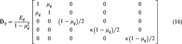
With this substitution, equation (17) takes the form

$${\overline{\mathbf{K}}}^e={\displaystyle \sum _{q=1}^n{\displaystyle {\int }_{-1}^1{\displaystyle {\int }_{-1}^1{\displaystyle {\int }_{-1}^1{\overline{\mathbf{B}}}^{\text{T}}{\overline{\mathbf{D}}}_q\overline{\mathbf{B}}\left|\mathbf{J}\right|\frac{h_q}{\eta }\text{d}r\text{d}s\text{d}{t}_q}}}}$$

(20)

where n is the total number of layers in the laminate.

Assemble of element matrixes

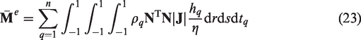
Element matrixes under local coordinate system need firstly to be transferred into global coordinate system and then assemble into the global matrixes. There are two kinds of matrix to be assembled: the element stiffness matrix and the element mass matrix. The procedure to obtain element stiffness matrix of laminate is presented in Section ‘Geometry of a degenerated shell element’. Now, we would like to show how to obtain the element mass matrix. There are two methods to calculate the element mass matrix, they are consistent mass matrix and lumped mass matrix. Consistent mass matrix is calculated here to ensure the consistence and accuracy. The general consistent mass matrix is expressed as

$${\overline{\mathbf{M}}}^e={\displaystyle {\int }_{\text{vol}.}\rho {\mathbf{N}}^{\text{T}}\mathbf{N}\text{d}x\text{d}y\text{d}}z={\displaystyle {\int }_{\text{vol}.}\rho {\mathbf{N}}^{\text{T}}\mathbf{N}\left|\mathbf{J}\right|\text{d}r\text{d}s\text{d}}t$$

(21)

where $\rho$ denotes the density and N denotes the shape function matrix. N is given by

$$\begin{array}{c}\mathbf{N}=\left[\begin{array}{cccc}{\mathbf{N}}_1& {\mathbf{N}}_2& {\mathbf{N}}_3& {\mathbf{N}}_4\end{array}\right]\\ {\mathbf{N}}_k=N^k{\mathbf{I}}_6\hspace{1em}\left(k=1,2,3,4\right)\end{array}$$

(22)

where $N^k$ is defined by equation (2) and I₆ is a (6 × 6) unit matrix. For the laminated structure, equation (21) can be rewritten as follows according to equation (18) and equation (19), i.e.

$${\overline{\mathbf{M}}}^e={\displaystyle \sum _{q=1}^n{\displaystyle {\int }_{-1}^1{\displaystyle {\int }_{-1}^1{\displaystyle {\int }_{-1}^1{\rho }_q{\mathbf{N}}^{\text{T}}\mathbf{N}\left|\mathbf{J}\right|\frac{h_q}{\eta }\text{d}r\text{d}s\text{d}{t}_q}}}}$$

(23)

where ${\rho }_q$ is the material density of layer q.

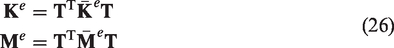
The element stiffness and mass matrix need to be transferred into global coordinate system. From equation (13), ${\mathbf{U}}^e$ is a mixed coordinates displacement, i.e. the displacement along axes is defined in global coordinate system and the rotation in axes is defined in local coordinate system. Thus, only the second half of each ${\mathbf{U}}_{\mathit{k}}^e$ needs to be transferred to global coordinates. Accordingly, we construct the following transform matrix:

$$\begin{array}{l}\mathbf{T}=\text{diag}\left(\begin{array}{cccc}\Lambda & \Lambda & \Lambda & \Lambda \end{array}\right)\\ \Lambda =\text{diag}\left(\begin{array}{cc}{\mathbf{I}}_3& \Theta \end{array}\right)\end{array}$$

(24)

where $\Theta$ is the matrix of direction cosines defined in equation (7) and ${\mathbf{I}}_3$ is a (3 × 3) unit matrix. So, the displacement under global coordinate is obtained

$${\mathbf{U}}^e=\mathbf{T}{\tilde{\mathbf{U}}}^e$$

(25)

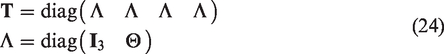
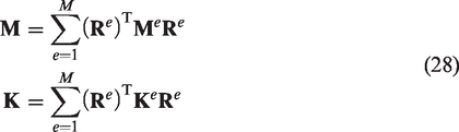
Similarly, the stiffness matrix and mass matrix under global coordinate are

$$\begin{array}{l}{\mathbf{K}}^e={\mathbf{T}}^{\text{T}}{\overline{\mathbf{K}}}^e\mathbf{T}\\ {\mathbf{M}}^e={\mathbf{T}}^{\text{T}}{\overline{\mathbf{M}}}^e\mathbf{T}\end{array}$$

(26)

Suppose $\mathbf{U}={\left\{{\mathbf{U}}_1{\mathbf{U}}_2\cdots {\mathbf{U}}_N\right\}}^{\text{T}}$ is the total displacement vector of all the nodes, where ${\mathbf{U}}_k={\left\{\begin{array}{l}{u}^k{v}^k{w}^k{\alpha }^k{\beta }^k{\gamma }^k\hfill \end{array}\right\}}^{\text{T}}\left(k=1,\mathrm{2\dots }N\right)$ , N is the number of all the nodes. The relation between $\mathbf{U}$ and ${\mathbf{U}}^e$ is defined by

$$\mathbf{U}={\mathbf{R}}^e{\mathbf{U}}^e$$

(27)

where ${\mathbf{R}}^e$ is a (6 × 6N) relationship matrix which is related to the $e\text{th}$ element. Suppose the node number of element e is i, j, m and p (seen in Figure 5), we can simply set the i, j, m and p columns of a (6 × 6N) matrix to be unit and others to be zero to construct the relationship matrix. Then, the assembled global stiffness and mass matrixes are

$$\begin{array}{l}\mathbf{M}={\displaystyle \sum _{e=1}^M{\left({\mathbf{R}}^e\right)}^{\text{T}}{\mathbf{M}}^e{\mathbf{R}}^e}\\ \mathbf{K}={\displaystyle \sum _{e=1}^M{\left({\mathbf{R}}^e\right)}^{\text{T}}{\mathbf{K}}^e{\mathbf{R}}^e}\end{array}$$

(28)

where M is the number of elements, M and K are call assembled mass matrix and assembled stiffness matrix, respectively.

Figure 5.

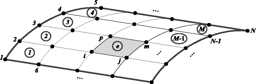
The numbering of nodes and elements.

Dynamic response analysis

The dynamic response analysis is a critical step for FEMilS. It is conducted by solving the dynamic equation of the FE model. The actuators and sensors can be viewed as additional mass, stiffness and damping matrixes to the FE model. Since for a light coil actuator, the influence of the coupling effect is non-significant, the additional effect can sometimes be neglected. The dynamic behavior of the FE cylindrical structure is governed by the following semi-discretization matrix differential equation set:

$$\mathbf{M}\ddot{\mathbf{U}}\left(t\right)+\mathbf{C}\dot{\mathbf{U}}\left(t\right)+\mathbf{KU}\left(t\right)\text{=}\mathbf{F}\left(t\right)$$

(29)

where U(t) is the time-dependent global displacement of all nodes, M, C and K are the mass, damping and stiffness matrix. Since solving the dynamic response of an FE model is computational-intensive, a reduced in-loop model is considered, i.e. some interested transfer paths can be extracted using block matrix. We assume that the input dimension is I, the dominating modal shape dimension is M and the output dimension is O, then the reduced (M × 1) dimensional modal force vector can be defined as

$${\mathbf{Q}}_{\text{r}}\left(t\right)={\mathbf{\Phi }}_{\text{ri}}^{\text{T}}{\mathbf{F}}_{\text{r}}\left(t\right)$$

(30)

where the subscript r denotes reduced and the number outside the bracket denotes dimensions of the vectors or matrixes. ${\mathbf{\Phi }}_{\text{ri}}^{\text{T}}$ is the reduced (M × I) dimensional modal matrix. ${\mathbf{F}}_{\text{r}}(t)$ is the reduced (I × 1) dimensional force vector. So the number of the modal equations is reduced to M, i.e.

$${\mathbf{M}}_{\text{pr}}{\ddot{\mathbf{\eta }}}_{\text{r}}\left(t\right)+{\mathbf{C}}_{\text{pr}}{\dot{\mathbf{\eta }}}_{\mathbf{r}}\left(t\right)+{\mathbf{K}}_{\text{pr}}{\mathbf{\eta }}_{\mathbf{r}}\left(t\right)={\mathbf{Q}}_{\text{r}}\left(t\right)$$

(31)

where ${\mathbf{M}}_{\text{pr}}$ , ${\mathbf{C}}_{\text{pr}}$ and ${\mathbf{K}}_{\text{pr}}$ are the (M × M) dimensional reduced modal mass, damping and stiffness matrix, respectively; ${\mathbf{\eta }}_{\mathbf{r}}(t)$ is the (M × I) dimensional reduced modal displacement vector.

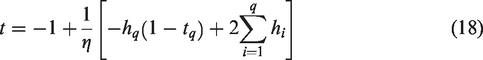
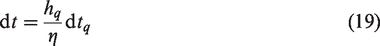
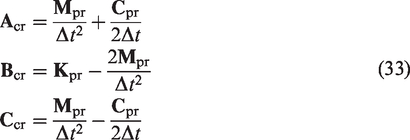
Considering that the input is an arbitrary signal, the classical Duhamel integral demands an integral from 0 to t every time instant, the computational complexity will increase with time. Therefore, we apply a recurrent method (central difference method) to overcome the computation accumulation problem and the solution of equation (31) is

$${\mathbf{\eta }}_{\mathbf{r}}\left(t\right)=\frac{{\mathbf{A}}_{\text{cr}}}{-{\mathbf{B}}_{\text{cr}}{\mathbf{\eta }}_{\mathbf{r}}\left(t-\Delta t\right)-{\mathbf{C}}_{\text{cr}}{\mathbf{\eta }}_{\mathbf{r}}\left(t-2\Delta t\right)+{\mathbf{Q}}_{\text{r}}\left(t-\Delta t\right)}$$

(32)

where

$$\begin{array}{l}{\mathbf{A}}_{\text{cr}}=\frac{{\mathbf{M}}_{\text{pr}}}{\Delta t^2}+\frac{{\mathbf{C}}_{\text{pr}}}{2\Delta t}\\ {\mathbf{B}}_{\text{cr}}={\mathbf{K}}_{\text{pr}}-\frac{2{\mathbf{M}}_{\text{pr}}}{\Delta t^2}\\ {\mathbf{C}}_{\text{cr}}=\frac{{\mathbf{M}}_{\text{pr}}}{\Delta t^2}-\frac{{\mathbf{C}}_{\text{pr}}}{2\Delta t}\end{array}$$

(33)

are (M × M) dimensional differential coefficient matrixes, and $\Delta t$ is a time interval that is related to sampling frequency. The input has the same definition as equation (30), so the real space response can be obtained by

$${\mathbf{U}}_{\text{r}}(t)={\mathbf{\Phi }}_{\mathbf{r}\text{o}}{\mathbf{\eta }}_{\mathbf{r}}(t)$$

(34)

where ${\mathbf{U}}_{\text{r}}(t)$ is the (O × 1) dimensional reduced output matrix. ${\mathbf{\Phi }}_{\mathbf{r}\text{o}}$ is the (O × M) dimensional modal matrix. Since the input and output dimensions are far smaller than the total dimensions, the subsystem reduction can tremendously reduce the computational complexity. A few low-order modes are usually dominating, so the computational speed improvement by modal reduction is also significant.

Numerical implementation

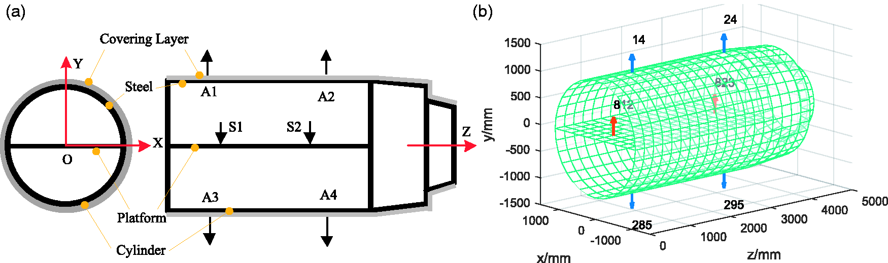
As a specific case, a laminated cylindrical structure with a platform inside, as illustrated in Figure 6(a), is considered. The materials of cylinder are steel and covering layer. The material of platform is steel. The axial direction of the cylinder is defined as z-axis and the x–y section is perpendicular to z-axis. The length of the cylinder is 4830 mm, and the maximum radius of the cylinder is 1100 mm. The engineering parameters of the cylindrical structure are listed in Table 1. The geometrical model and its mesh are illustrated using MATLAB, as shown in Figure 6(b). The cylinder is divided into 32 × 22 rectangle elements and the platform is divided into 10 × 15 rectangle elements. Thus, the cylinder has 32 nodes in circumferential direction (x–y section) and 23 nodes in z-axis, and the platform has 11 nodes in x-axis and 16 nodes in z-axis. Adjacent two elements share two nodes, and the adjacent three elements where cylinder and platform is connected share two nodes, so there are 880 nodes in total. Each node has six DOFs, so the total DOFs are 5280, if the cylinder is unconstrained. The xyz translations of each node are considered to be main DOFs of the system, thus reducing the total DOFs to 2640. In Figure 6, node 14 (A1), node 24 (A2), node 285 (A3), node 295 (A4), node 812 (S1) and node 823 (S2) are chosen as observation point.

Figure 6.

The sketch and mesh of the cylindrical structure.

Table 1.

Parameters of the cylindrical structure.

Parameters	Steel	Covering layer
Thickness	60 mm	60 mm
Elastic modulus	2 × 105 MPa	8 MPa
Poisson’s ratio	0.3	0.45
Density	7.85 × 10–9 tonne/mm3	1.28 × 10–9 tonne/mm3

Modal analysis of the above model is conducted using MATLAB. Modal shape displacement is stored in column of the modal matrix, which is obtained by solving eigen-problem using global mass and stiffness matrix. We add the modal shape displacement to each node of the cylinder and platform and then obtained 3D illustration of the modal shape. For a better visualization, longitudinal-section and cross-section of the model are also illustrated. Since the model is unconstrained, rank 1 to rank 6 are rigid body freedom modes. The 3D illustration, longitudinal-section illustration and cross-section illustration of rank 7, 8, 10, 11, 13 are, respectively, illustrated in Figure 7(a1) to (a3), (b1) to (b3), (c1) to (c3), (d1) to (d3) and (e1) to (e3). It can be seen from the figures that the platform can be viewed as a plate whose edges in z-axis are clamped and edges in x-axis are free. In direction of z-axis, the mode of platform is similar to free–free beam, thus the translation, 1st bending and 2nd bending modes of platform occur in rank 8, 10, and 13, respectively, of the whole structure. In the direction of x-axis, the mode of platform is similar to clamped-clamped beam, the 1st bending mode occurs in multiple ranks (8, 10 and 13) of whole structure. It can also be seen for the figures that one end of the cylinder has very large stiffness, and its behavior in z-axis is similar to clamped-free beam, thus the 1st bending, 2nd bending and 3rd bending modes occur in rank 7/8, 10 and 13, respectively, of the whole structure. In x–y section, the 1st bending, 2nd bending, 3rd bending and 4th bending occur in rank 7, 8/10, 12 and 13, respectively, of the whole structure. The twist modes of platform and cylinder occur in rank 11 of the whole structure. In rank 7, the platform does not have local modes, and the displacement in platform is caused by cylinder deformation. The modes of platform and cylinder are summarized in Table 2.

Figure 7.

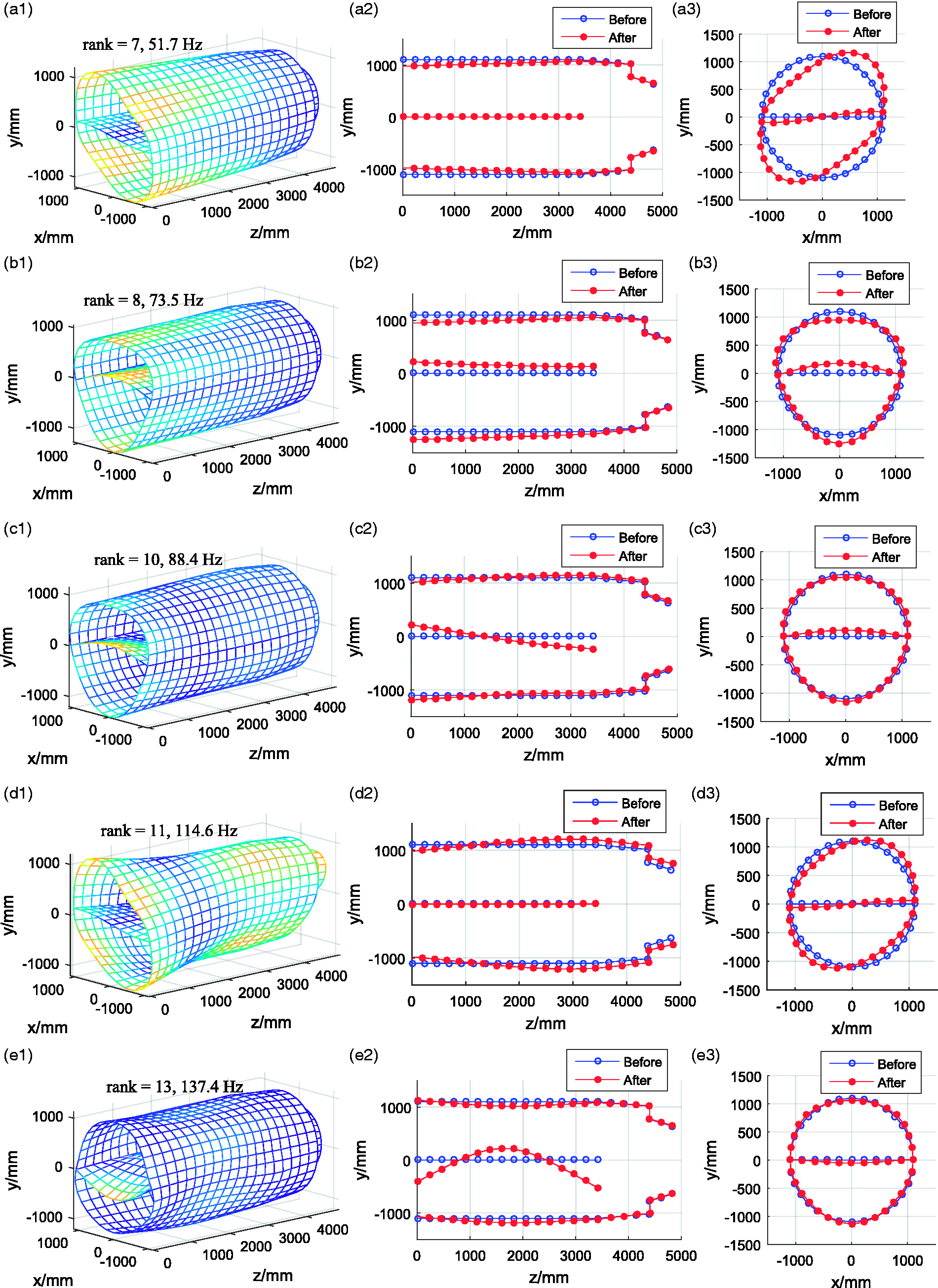
The 3D illustration, longitudinal-section illustration and cross-section illustration of the modal shape: (a1) to (a3) rank 7, (b1) to (b3) rank 8, (c1) to (c3) rank 10, (d1) to (d3) rank 11, and (e1) to (e3) rank 13.

Table 2.

Modes of platform and cylinder.

Rank	Platform		Cylinder
	z-axis	x-axis	z-axis	xy-plane
7	–	–	1st bending	1st bending
8	translation	1st bending	1st bending	2nd bending
10	1st bending	1st bending	2nd bending	2nd bending
11	1st twist	1st twist	1st twist	1st twist
13	2nd bending	1st bending	3rd bending	4th bending

The harmonic response analysis has also been conducted. We give harmonic excitation in nodes 812, 823, 14 and 24, respectively, and then collect the amplitude of steady-state response of all nodes. After that we add the amplitude to the nodes and give 3D illustration to see the amplitude distribution of the cylinder. For all the four cases, the excitation input is 20 Hz unit sinusoidal force in radial direction. According to the linear system theory, the response of each node is 20 Hz sinusoidal wave with different amplitudes and initial phases. Figure 8(a1) to (a2), (b1) to (b2), (c) and (d) shows the response distribution when excitation at node 812, 823, 14, and 24, respectively. The vibration deformations of each node in Figure 8 are decided by the amplitude of the sinusoidal responses and the directions of that are decided by the initial phase of the responses. It can be seen from the figure that (1) the amplitude is larger near excitation point; (2) there are nodal lines on the cylinder and the vibration directions are opposite on different sides of the nodal lines.

Figure 8.

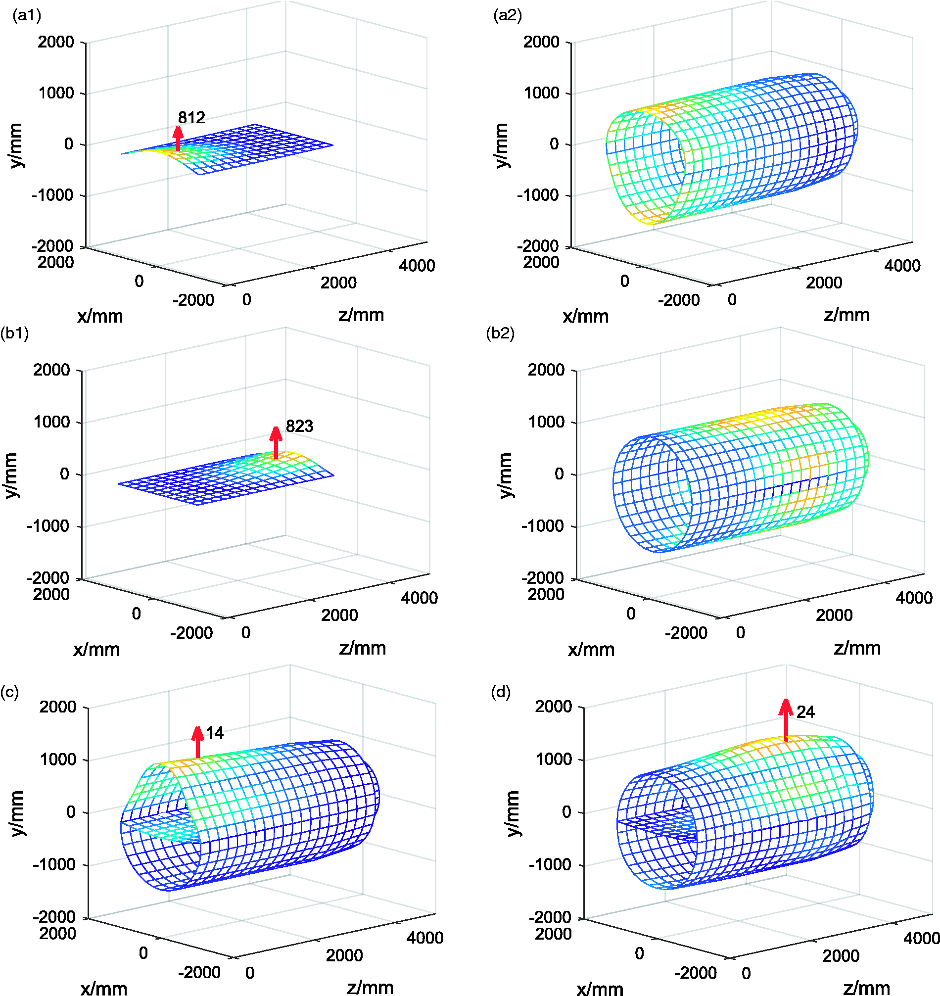
Harmonic response analysis: (a1 and a2) excitation on platform, node 812; (b1 and b2) excitation on platform, node 823; (c) excitation on cylinder, node 14; (d) excitation on cylinder node 24.

AVC case study on FEMilS

Formulation of MIMO adaptive algorithm

Narrowband FXLMS (NFXLMS) algorithm is specialized for the multiple frequency and multiple source vibration control. The NFXLMS will be extended to MIMO using matrix representation.

As shown in Figure 9, we consider J primary sources, K secondary sources and M error sensors, in which the ith primary source contains $I_j$ frequency component. For NFXLMS algorithm, all the frequencies of all the sources can be combined into one (I × 1) dimensional column vector to generate reference signals, i.e.

$${\mathbf{\omega }}_{\text{r}}={\left\{{\omega }_{\text{r,}i}\right\}}^T,i=1,2,\mathrm{\dots },I$$

(35)

where $I={\displaystyle {\sum }_{j=1}^J{I}_j}$ . Accordingly, two (I × 1) dimensional reference vectors can be defined as

$${\mathbf{x}}_{\text{c}}\left(n\right)={\left\{x_{\text{c},i}\left(n\right)\right\}}^T=\cos {\mathbf{\omega }}_{\text{r}},{\mathbf{x}}_{\text{s}}\left(n\right)={\left\{x_{\text{s},i}\left(n\right)\right\}}^T=\sin {\mathbf{\omega }}_{\text{r}},i=1,2,\mathrm{\dots },I$$

(36)

Figure 9.

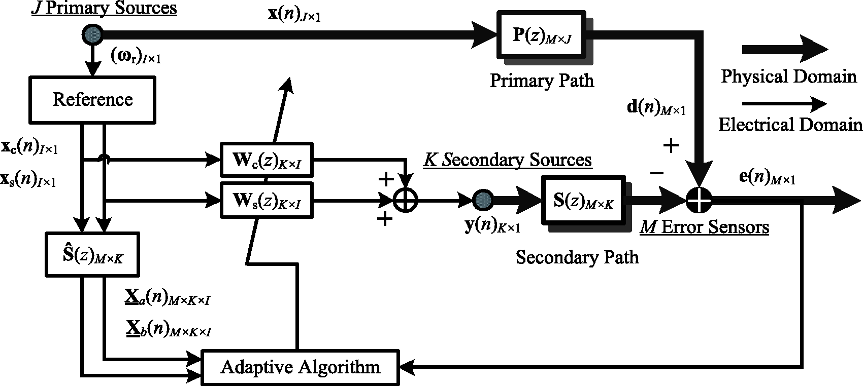
Diagram of MIMO-NFXLMS system.

For each secondary source and each frequency component, there will be two coefficients in the controller. Thus, the controller coefficients can be defined as two (K × I) dimensional matrixes, i.e.

$${\mathbf{W}}_{\text{c}}\left(n\right)=\left[w_{\text{c},\mathit{ki}}\left(n\right)\right],{\mathbf{W}}_{\text{s}}\left(n\right)=\left[w_{\text{s},\mathit{ki}}\left(n\right)\right],k=1,2,\mathrm{\dots },K,i=1,2,\mathrm{\dots },I$$

(37)

where $w_{\text{c},\mathit{ki}}(n)$ and $w_{\text{s},\mathit{ki}}(n)$ denote the controller coefficients for the kth secondary source and the ith frequency component. The output of the controller can be expressed as

$$\mathbf{y}\left(n\right)={\mathbf{W}}_{\text{c}}\left(n\right){\mathbf{x}}_{\text{c}}\left(n\right)+{\mathbf{W}}_{\text{s}}\left(n\right){\mathbf{x}}_{\text{s}}\left(n\right)$$

(38)

where $\mathbf{y}(n)$ is the (K × 1) dimensional vectors. The error signals are superposition of primary noises and secondary noises, i.e.

$$\mathbf{e}\left(n\right)=\mathbf{d}\left(n\right)-\mathbf{S}\left(n\right)\ast \mathbf{y}\left(n\right)$$

(39)

where $\mathbf{e}(n)$ denotes (M × 1) dimensional error vector, $\mathbf{d}(n)$ denotes (M × 1) dimensional primary noise vector, $\mathbf{S}(n)$ denotes (M × K) dimensional impulse response function matrix of secondary path, in which the element $s_{\mathit{mk}}(n)$ denotes the impulse response function from the kth secondary source to the mth error sensor, and * denotes linear convolution. The filtered reference signals are also required for the controller coefficients updating. They are (M × K×I) dimensional matrixes. We use underline to distinguish three-dimensional matrix from the two-dimensional one, i.e.

$${{\underset{¯}{\mathbf{X}}}^{\mathbf{\prime }}}_{\text{c}}\left(n\right)=\widehat{\mathbf{S}}\left(n\right)\ast {\mathbf{x}}_{\text{c}}\left(n\right),{{\underset{¯}{\mathbf{X}}}^{\mathbf{\prime }}}_{\text{s}}\left(n\right)=\widehat{\mathbf{S}}\left(n\right)\ast {\mathbf{x}}_{\text{s}}\left(n\right)$$

(40)

where $\widehat{\mathbf{S}}(n)$ denotes the estimation of $\mathbf{S}(n)$ . According to the stochastic descent method, the updated equation of the controller coefficient can be expressed as

$${\mathbf{W}}_l\left(n+1\right)={\mathbf{W}}_l\left(n\right)+{\mu }_l{{\underset{¯}{\mathbf{X}}}^{\mathbf{\prime }}}_l^T\left(n\right)\mathbf{e}\left(n\right),l=\text{c},s$$

(41)

where ${{\underset{¯}{\mathbf{X}}}^{\mathbf{\prime }}}_l^T$ is the transpose of ${\hspace{0.17em}}_{{\underset{¯}{\mathbf{X}}}^{\mathbf{\prime }}}^l$ , i.e. a (K × I×M) dimensional matrix.

The AVC case study

The layout of the FEMilS is shown in Figure 10. Node 812 and node 823 are selected to be primary vibration source point, i.e. the primary vibration will be injected to the model from these two nodes. Nodes 14, 24, 285 and 295 are selected to be control point, i.e. actuating forces will be injected to the model from these nodes and responses will be measured from these nodes. In the control process, the primary vibration and the control actuating forces are injected simultaneously to the system point-by-point and the real-time feedback and feedforward signal are obtained to the controller, thus the control forces can be calculated timely.

Figure 10.

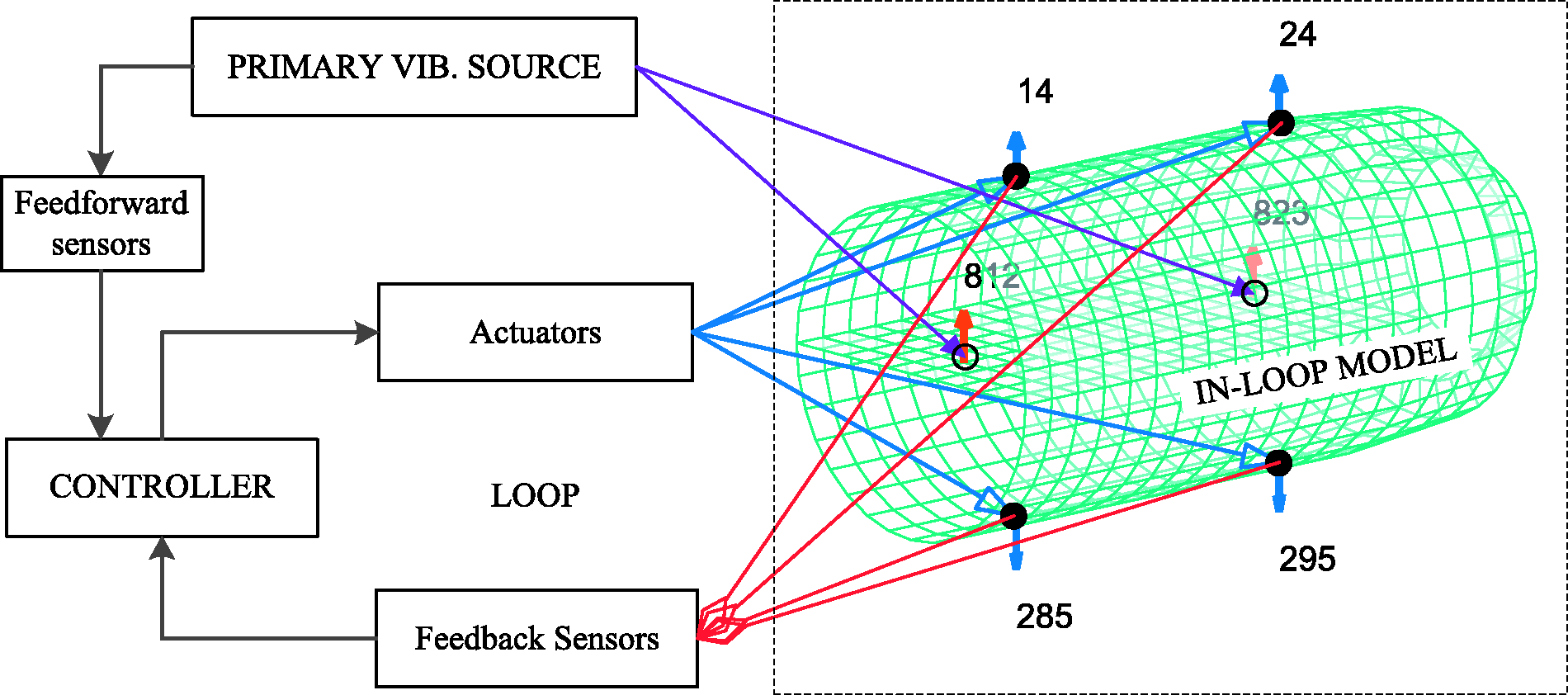
Layout of the FEMilS.

Four AVC cases based on the MIMO adaptive algorithm and FEMilS are conducted. They are SFSS-SISO (single frequency, single source, single input and single output), MFSS-SISO (multiple frequencies, single source, single input and single output), MFSS-MIMO (multiple frequencies, single source, multiple inputs and multiple outputs) and MFMS-MIMO (multiple frequencies, multiple sources, multiple inputs and multiple outputs). The simulation parameters are listed in Table 3. The simulation results are shown in Figures 11 to 14.

Table 3.

Parameters of simulation.

Case	Sampl. freq. (Hz)	Sampl. time (s)	Primary freq. (Hz)	Primary force (N)	Noise (%)	Source position	Control position
Case A:SFSS-SISO	2048	2	30	600	0	S1 (node 812)	A1 (node 14)
Case B:MFSS-SISO	2048	5	20,40,60	200,100,150	20	S1 (node 812)	A1 (node 14)
Case C:MFSS-MIMO	2048	10	20,40,60	200,100,150	20	S1 (node 812)	A1, A4 (nodes 14, 295)
Case D:MFMS-MIMO	2048	40	20,40,6035,70	400,200,100400,100	20	S1, S2 (nodes 812, 823)	A1, A2, A3, A4(nodes 14, 24, 285, 295)

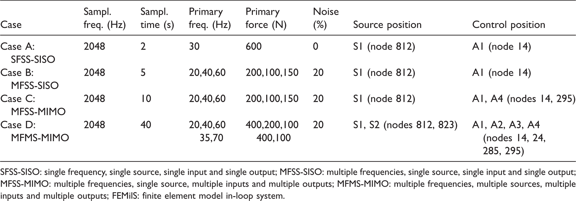
SFSS-SISO: single frequency, single source, single input and single output; MFSS-SISO: multiple frequencies, single source, single input and single output; MFSS-MIMO: multiple frequencies, single source, multiple inputs and multiple outputs; MFMS-MIMO: multiple frequencies, multiple sources, multiple inputs and multiple outputs; FEMilS: finite element model in-loop system.

Case A: SFSS-SISO

The simulation with single primary source (node 812), single frequency (30 Hz), single input (node 14) and single output (node 14) is considered in case A. The sampling frequency is 2048 Hz; sampling time is 2 s; frequency component of primary noise is 600sin(60πt); the in-loop model is a model with 2-input, 1-output, and 16 dominating modes; the step-size is 1e9. The primary (source vibration) and secondary forces (actuating force) are shown in Figure 11(a) and (b), respectively. The responses at node 14 with control on and off are shown in Figure 11(c). The controller coefficients are shown in Figure 11(d). It can be seen from the figures that with the secondary force and the controller coefficient going to steady-state, the response are dramatically suppressed.

Figure 11.

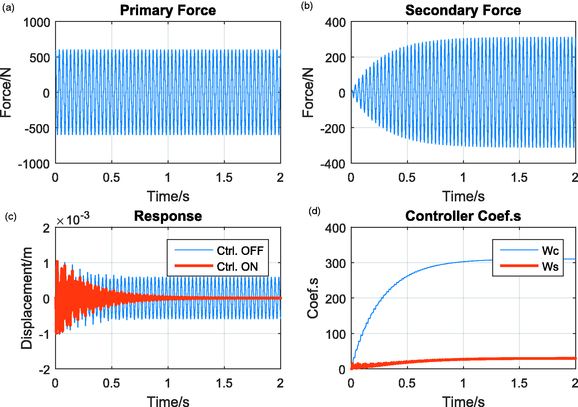
Case 1: single frequency, single source, single input and single output (SFSS-SISO) control based on FEMilS.

Case B: MFSS-SISO

The simulation with single primary source (node 812), multiple frequencies (20 Hz, 40 Hz and 60 Hz), single input (node 14) and single output (node 14) is considered in case B. The sampling frequency is 2048 Hz; sampling time is 5 s; multiple frequency components of primary noise are 200sin(40πt), 100sin(80πt), 150sin(120πt) and 20% colored noise; the in-loop model is a model with 2-input, 1-output, and 16 dominating modes; the step-size is 2e8. The primary excitation force containing three harmonic components and colored noise is shown in Figure 12(a). The secondary forces are shown in Figure 12(b). It can be seen that the control force containing multiple frequency components goes to state-state quickly. The responses in time and frequency domain are, respectively, shown in Figure 12(c) and (d). It can be seen that (1) in time domain the response quickly suppressed with control on, remaining some broadband noise; (2) in frequency domain, the main line spectral components are clearly cancelled.

Figure 12.

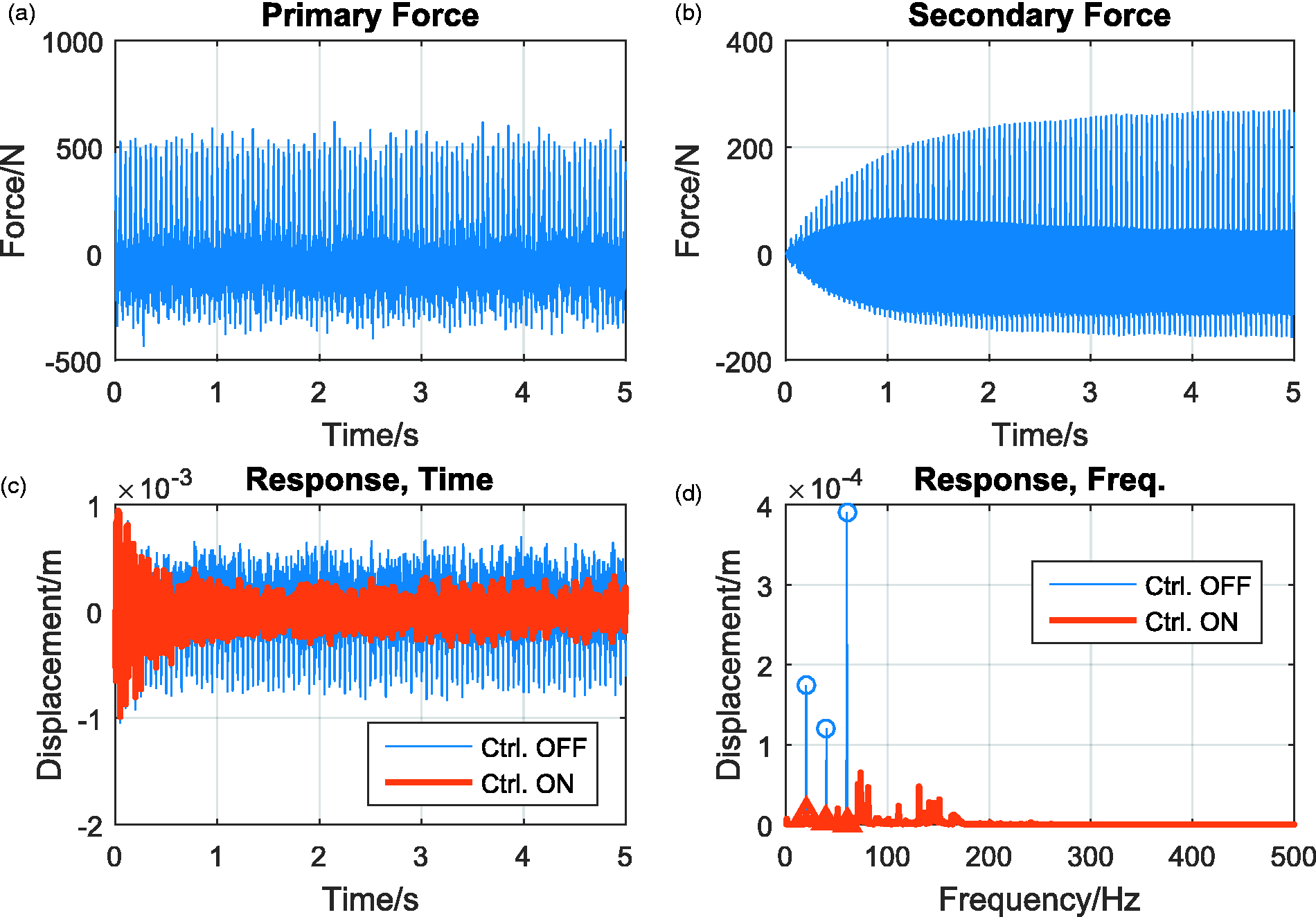
Case 2: multiple frequencies, single source, single input and single output (MFSS-SISO) control based on FEMilS.

Case C: MFSS-MIMO

The simulation with single primary source (node 812), multiple frequencies (20 Hz, 40 Hz and 60 Hz), multiple inputs (node 14, 295) and multiple outputs (node 14, 295) is considered in case C. The sampling frequency is 2048 Hz, sampling time is 10 s; multiple frequency components of primary noise is 200sin(40πt), 100sin(80πt), 150sin(120πt) and 20% colored noise; the in-loop model is a model with 3-input, 2-output, and 16 dominating modes; the step-size is 1e8 and 4e8. The primary force is shown in Figure 13(a). The secondary forces are shown in Figure 13(b), where A1 is the excitation at node 14, A4 is the excitation at node 295. It can be seen from the figure that the control force at A4 is smaller than that at A1. This is because that A4 is further from the vibration source S1 than A1. The time domain response of A1 and A4 is shown in Figure 13(c) and (d), respectively. It can be seen that the time domain response dramatically suppressed with control on. The frequency domain response of A1 and A4 are shown in Figure 13(e) and (f), respectively. It can be seen that the dominating line spectrum can be clearly cancelled.

Figure 13.

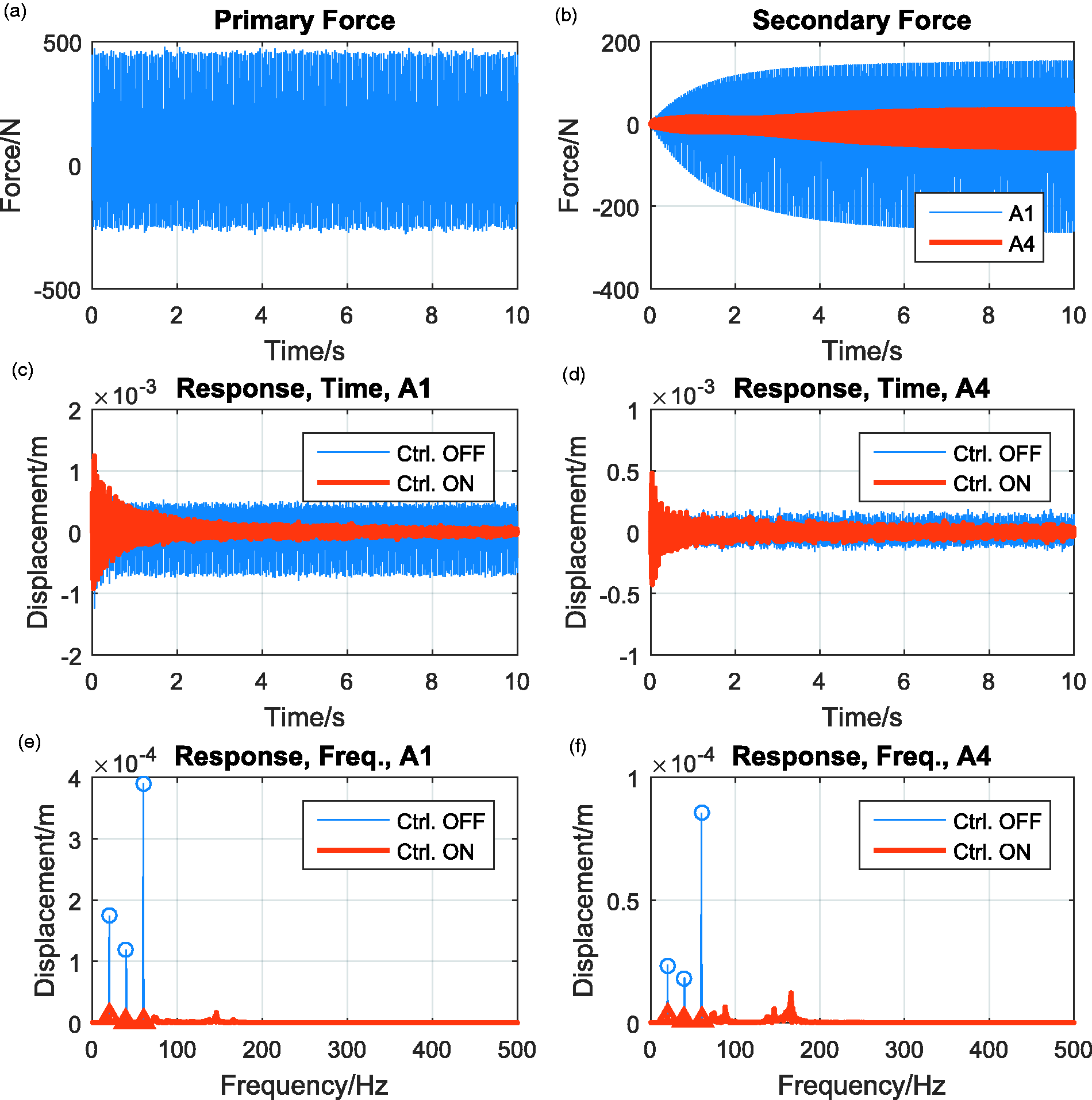
Case 3: multiple frequencies, single source, multiple inputs and multiple outputs (MFSS-MIMO) control based on FEMilS.

Case D: MFMS-MIMO

The simulation with multiple primary sources (node 812, 823), multiple frequencies (20 Hz, 40 Hz and 60 Hz; 35 Hz, 70 Hz), multiple inputs (node 14, 24, 285 and 295) and multiple outputs (node 14, 24, 285 and 295) is considered in case D. The simulation sampling frequency is 2048 Hz, sampling time is 40 s; multiple frequency components of primary noise S1 are 400sin(40πt), 200sin(80πt), 100sin(120πt) and 20% colored noise; multiple frequency components of primary noise S2 are 400sin(70πt), 100sin(140πt) and 20% colored noise; the in-loop model is a model with 6-input, 4-output, and 16 dominating modes; the step-sizes are 5e7, 1e8, 1e7 and 1e8. The control force on A1 and A2 is shown in Figure 14(b1) and that of A3 and A4 are shown in Figure 14(b2). It can be seen that (1) the control is off before 15 s (i.e. the control forces are zero before 15 s); (2) all the four control forces goes to steady state around 30 s. The time domain responses of A1, A2, A3 and A4 are shown in Figure 14(c1), (c2), (c3) and (c4), respectively. It can be seen from the figures that the response is very large before 15 s and it quickly die out after 15 s, leaving alone a few broad band noise. The frequency domain of the four control points is shown in Figure 14(d1), (d2), (d3) and (d4), respectively. The data of control off and control on are extracted from the time period of 12–14 s and 38–40 s, respectively, of the response signals. It can be seen from the figures that all the frequencies at all the control point can be effectively suppressed.

Figure 14.

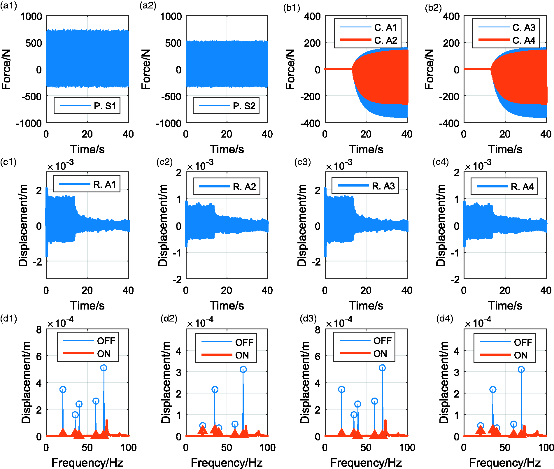
Case 4: multiple frequencies, multiple sources multiple inputs and multiple outputs (MFMS-MIMO) control based on FEMilS.

Conclusion

In this paper, we propose an effective FEMilS for MIMO AVC. An effective FE model of laminated thick cylindrical structure with four-node Mindlin degenerated shell element has been applied. The numerical modal analysis, harmonic response analysis of the cylinder has been conducted by MATLAB to verify the correctness and accuracy of the model. An MFMS-MIMO adaptive algorithm has been realized based on the FEMilS. Numerical AVC investigations have been carried out on a variable section cylindrical structure model with a rectangle plane. It can be concluded from the results that (1) the algorithm can individually and effectively suppress each component of the multiple frequency vibration; (2) the FEMilS is convenient and straightforward for multiple sources, multiple inputs and multiple outputs with an acceptable loop time. We believe that with the development of the computer technology, large scale FE model in-loop simulation will make an increasing contribution to the study of AVC.