A new approach toward damage localization and quantification of structures under changing temperature condition

Abstract

Most damage detection methods developed in the literature cannot give the locations and extent of damages under the presence of varying temperature condition. This is because temperature condition changes the vibration properties of a structure, which are commonly analyzed for damage detection, and temperature gradient throughout the structure makes it difficult to create a baseline for the undamaged structure, as the baseline is generally constructed using features obtained under a wide range of temperature conditions. In this paper, a new insight on how to approach damage detection using only a single temperature condition to create the baseline is proposed. This approach solves the damage detection under changing temperature problem in two stages by first quantifying the change of stiffness of all the elements in a structure due to temperature and damage effects, followed by removing the temperature effect, a global effect, to give the actual damage locations and extent. Using single temperature condition allows new measurements to be compared to a benchmark so that local deviation can be obtained, thus making the damaged elements identifiable. The proposed approach is tested using a beam structure model and a shear building under different gradient temperature conditions, and the results demonstrate that the method successfully eliminates the change in elemental stiffness due to temperature effect and gives correct damage locations and extent. The approach can be implemented with other existing damage detection methods that did not consider the effect of temperature so that structures under varying temperature condition can be analyzed.

Introduction

Engineering structures in general are subjected to constant degradation due to the harsh environmental and operational conditions they are faced with. To maintain their safety and reliability, researchers have been developing damage detection methods^1–4 to assess the health condition of the structures to allow reparation/replacement of structural defects at an early stage before catastrophic failure occurs. Based on the information given on the state of damages, the damage detection methods can be classified into four different levels as given by Rytter ⁵

Level 1: Detect the presence of damages only in the structure.

Level 2: Detect and give the locations of damages in the structure.

Level 3: Detect, locate, and give the extent of damages in the structure.

Level 4: Detect, locate, and quantify damages, and give the level of safety of the structure depending on the damage case.

In the literature, several level 2^1,2,6 and level 3^1,2,7 damage detection methods have been proposed and applied to numerical and experimental structures. However, most of the proposed methods were verified by assuming that the environmental conditions the structures are faced with are constant. ⁸ Yet, it is well known that the changing environmental conditions, the changing temperature condition in particular, have a major influence on the dynamic properties of civil engineering structures, ⁹ which are commonly used as damaged sensitivity features for damage detection. As a result, false alerts may occur. Thus, to provide a robust damage detection method, which does not give false alerts, the effects of the changing environmental conditions, especially the changing temperature condition, should be taken into consideration while deriving the method. ¹⁰ Moreover, the temperature condition usually has nonlinear effect on the dynamic properties of the structures, ¹¹ and temperature gradient throughout the structures usually exists, ¹⁰ both of which also need to be considered in the development of the damage detection method.

To tackle this temperature condition issue, several approaches, such as regression analysis^12–14 and the use of multivariate statistical tools^11,14,15 to process the damage sensitivity features, have been proposed in the literature; however, most of these approaches can only give the presence of damages in the structures. Among the proposed approaches, limited methods can perform level 2 of damage detection,^16–18 and only a few methods can perform level 3 of damage detection, i.e. give the presence, locations, and extent of the damages altogether,^10,19 yet most of the existing methods do not perform well under gradient temperature condition and under nonlinear effect of the changing temperature condition. The difficulties in the development of level 3 damage detection under changing temperature condition may be attributed to the unfit approach adopted by the researchers, as the methods proposed in the literature usually use the concept of creating the baseline of an undamaged structure using damage sensitivity features captured from a wide range of temperature conditions so as to cover all possible scenarios the structure may encounter,^8,20,21 and compare new measurements with the baseline to see whether they lie within the normal range. However, by doing so, a new measurement from the structure under a specific temperature distribution is only being compared to measurements from the undamaged structure under normal temperature conditions; it is not being compared to a benchmark that represents the undamaged structure at exactly the same temperature distribution. Therefore, it is generally difficult to determine which part of the structure differs from the one of the undamaged structure.

It is difficult to compare a new measurement captured at a specific temperature condition to the same condition from the undamaged structure because, as mentioned previously, structures are subjected to gradient temperature and to nonlinear temperature effect. These make obtaining the exact same temperature condition from the undamaged structure to be used as baseline difficult, because there is an infinite amount of temperature variations throughout the structure, and this is the main reason why new observations are only being compared to a set of undamaged measurements to see whether they behave similarly. To tackle this problem, some methods in the literature tried to predict the temperature condition along with the damage locations based on the features gathered; ¹⁰ however, gradient temperature distribution makes it difficult to get reasonable results because generally, only temperature at one or a few locations are measured throughout the whole structure, hence leading to errors in the temperature profile. Moreover, constructing the baseline from a wide range of temperature conditions has the drawback that it may reduce the sensitivity of the methods to detect small damages if proper consideration is not taken into account; ²² it is also time-consuming to gather all the necessary features for damage detection, hence retarding the implementation of the methods.

This paper proposes a new insight on how to approach damage detection under varying temperature condition by adopting only one temperature condition for the baseline of the undamaged structure. This approach first treats damage detection under changing temperature condition in the same way as one treats damage detection assuming constant temperature condition, followed by determining the change in stiffness of each element of the structure due to external effects. After the change in elemental stiffness has been quantified, temperature effect is removed from the extent coefficients by analyzing the trend of the extent coefficients along the structure to give damage locations and extent. In this paper, the damage detection method by Soo Lon Wah and Chen ²³ is further extended to take into account the effect of changing temperature with gradient temperature distribution. The proposed method uses frequency responses, and stiffness and degrees-of-freedom of each element to obtain an extent coefficient for each element to represent the effects of both temperature and damage on the structure. After the extent coefficients for all elements have been found, the temperature effect is then removed to give altogether the actual damage locations and damage extent calculated based on using one temperature as baseline. To demonstrate the proposed approach, a beam structure model and a shear building are used as examples for damage detection and quantification, and the results obtained show that by using only one temperature condition for the baseline, damage localization and quantification under gradient temperature condition and nonlinear temperature effect can be achieved. This approach can be implemented easily with other existing damage detection methods to tackle level 3 damage detection under varying temperature condition.

Damage detection methodology

This section introduces the proposed approach for damage detection, localization, and quantification of civil engineering structures subjected to varying temperature condition and to gradient temperature distribution. In this approach, damages in a structure are assumed to be represented by reductions in elemental stiffness of the members of the structure, and the locations of the damages are given by the element number each element is assigned to. The approach consists of two stages. In the first stage, an extent coefficient that is related to the contribution of the temperature and damage effects affecting the structure is assigned to each element present in the structure. In the second stage, the temperature effect is removed from the extent coefficient so that the damage extent can be obtained through the use of a damage coefficient. The damage coefficient, if not equals to zero, gives the actual damage extent of an element, and the location of the damage can be identified by the element number accordingly.

Stage 1: Extent coefficient assignment

Consider a structure with $\text{n}$ degrees-of-freedom subjected to a forced harmonic excitation. The mathematical model representing the motion of the structure can be given by the equation of motion

$$\mathbf{M}\ddot{\mathbf{X}}(\text{t})+\mathbf{C}\dot{\mathbf{X}}(\text{t})+KX(\text{t})=f{\text{e\hspace{0.17em}}}^{\text{j}\omega \text{t}}$$

(1)

where

M, C, and K are the $\text{n}\times \text{n}$ mass, damping, and stiffness matrices of the structure, respectively;

$X(\text{t})$ is the $\text{n}\times 1$ displacement response vector of the structure;

f is the $\text{n}\times 1$ amplitude vector of the forced harmonic excitation;

$\text{j}$ is the imaginary unit $(=\sqrt{-1})$ ;

ω is the angular frequency of the forced harmonic excitation.

For simplicity, the damping matrix C is neglected. Thus, equation (1) becomes

$$\mathbf{M}\ddot{\mathbf{X}}(\text{t})+KX(\text{t})=f{\text{e}}^{\text{j}\omega \text{t}}$$

(2)

Structural damage or structural change due to temperature variation here is referred to as a reduction/increase in the stiffness property of the structure with no change in the mass property. Hence, the equation of motion of the structure under the damage and temperature effects subjected to the same forced harmonic excitation can be given as

$$M{\ddot{\mathbf{X}}}_{\text{c}}(\text{t})+K_{\text{c}}{X}_{\text{c}}(\text{t})=f{\text{e}}^{\text{j}\omega \text{t}}$$

(3)

where

$K_{\text{c}}$ is the $\text{n}\times \text{n}$ stiffness matrix of the structure under the damage and temperature effects;

$X_{\text{c}}(\text{t})$ is the $\text{n}\times 1$ displacement response vector of the structure under the damage and temperature effects.

The stiffness matrix and the displacement response vector of the structure under the damage and temperature effects can be expanded and rewritten as

$$K_{\text{c}}=K-\delta K$$

(4a)

$$X_{\text{c}}=X-\delta X$$

(4b)

where

$\delta K$ represents the small change of the stiffness matrix due to damage and temperature effects;

$\delta X$ represents the small change of the displacement response vector due to damage and temperature effects.

Substituting equation (4) into equation (3) and noting equation (2) leads to

$$\mathbf{M}\delta \ddot{\mathbf{X}}(\text{t})+K\delta X(\text{t})+\delta K{X}_{\text{c}}(\text{t})=0$$

(5)

Since the input excitation is harmonic, the steady-state output will also be harmonic. Therefore, at steady state

$$X(\text{t})=Y{\text{e}}^{\text{j}\omega \text{t}}$$

(6a)

$$\delta X(\text{t})=\delta Y{\text{e}}^{\text{j}\omega \text{t}}$$

(6b)

$$X_{\text{c}}(\text{t})=Y_{\text{c}}{\text{e}}^{\text{j}\omega \text{t}}$$

(6c)

In which Y, $\delta Y$ , and $Y_{\text{c}}$ represent the $\text{n}\times 1$ steady-state vibration amplitudes of $X(\text{t}),\delta X(\text{t})$ , and $X_{\text{c}}(\text{t})$ , respectively.

Substituting equation (6) into equation (5) leads to equation (7), which is only valid for a specific excitation frequency ω.

$$(K-{\omega }^{\text{2}}M)\delta Y+\delta K{Y}_{\text{c}}=0$$

(7)

Rearranging yields

$$\delta K{Y}_{\text{c}}=({\omega }^{\text{2}}M-K)\delta Y$$

(8)

In which the left-hand side of the equation has an unknown term $\delta K$ which represents the change in global stiffness of the structure as a result of damage and temperature effects affecting the structure. This change is due to the reduction/increase in elemental stiffness of all the elements of the structure due to the temperature effect, and the reduction in elemental stiffness of all the damaged elements. It can be represented by

$$\delta K={\displaystyle \sum _{\text{s}\hspace{0.17em}=\hspace{0.17em}1}^{\text{TE}}{\text{c}}_{\text{s}}}{K}_{\text{s}}$$

(9)

where

$\text{TE}$ is the total number of elements in the structure;

$K_{\text{s}}$ is the elemental stiffness matrix of the $\text{sth}$ element at reference temperature;

${\text{c}}_{\text{s}}$ is the extent coefficient of the $\text{s}\text{th}$ element, which represents the percentage reduction/increase in stiffness of the element after the reduction/increase in stiffness due to the combination of damage and temperature effects, when compared to the original stiffness of the member obtained at reference temperature.

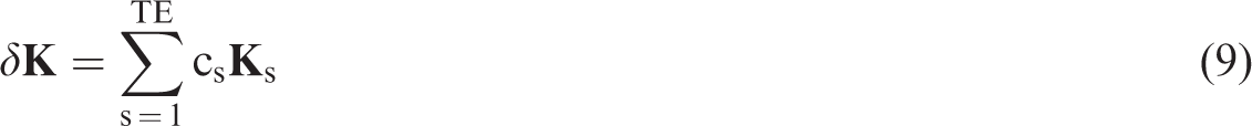
Substituting equation (9) into equation (8) yields

$$\left({\displaystyle \sum _{\text{s}=1}^{\text{TE}}{\text{c}}_{\text{s}}}{K}_{\text{s}}\right)Y_{\text{c}}=({\omega }^{\text{2}}M-K)\delta Y$$

(10)

Rearranging results into

$${\displaystyle \sum _{\text{s}=1}^{\text{TE}}{\text{c}}_{\text{s}}}{K}_{\text{s}}{Y}_{\text{c}}=({\omega }^{\text{2}}M-K)\delta Y$$

(11)

Equation (11) can be decomposed into $\text{n}$ number of equations, with each being expressed as

$${\displaystyle \sum _{\text{s}=1}^{\text{TE}}{\text{c}}_{\text{s}}}{K}_{\text{s,p}}{Y}_{\text{c}}={\text{v}}_{\text{p}}$$

(12)

where

$K_{\text{s,p}}$ is the $\text{pth}$ row in the elemental stiffness matrix of the $\text{sth}$ element;

${\text{v}}_{\mathrm{p}}$ is the $\text{pth}$ row of the $\text{n}\times 1$ vector v, where $v=({\omega }^{\text{2}}M-K)\delta Y$ .

Expanding equation (12) yields

$${\text{c}}_{\text{1}}{K}_{\text{1,p}}{Y}_{\text{c}}+{\text{c}}_{\text{2}}{K}_{\text{2,p}}{Y}_{\text{c}}+\cdots +{\text{c}}_{\text{TE}}{K}_{\text{TE,p}}{Y}_{\text{c}}={\text{v}}_{\text{p}}$$

(13)

Hence, similar to equation (13), the system of the $\text{n}$ number of equations due to the decomposition of equation (11) can be expressed as

$$\begin{array}{l}{\text{c}}_{\text{1}}{K}_{\text{1,1}}{Y}_{\text{c}}+{\text{c}}_{\text{2}}{K}_{\text{2,1}}{Y}_{\text{c}}+\cdots +{\text{c}}_{\text{TE}}{K}_{\text{TE,1}}{Y}_{\text{c}}={\text{v}}_{\text{1}}\hfill \\ {\text{c}}_{\text{1}}{K}_{\text{1,2}}{Y}_{\text{c}}+{\text{c}}_{\text{2}}{K}_{\text{2,2}}{Y}_{\text{c}}+\cdots +{\text{c}}_{\text{TE}}{K}_{\text{TE,2}}{Y}_{\text{c}}={\text{v}}_{\text{2}}\hfill \\ \hfill ⋮\hfill \\ {\text{c}}_{\text{1}}{K}_{\text{1,n}}{Y}_{\text{c}}+{\text{c}}_{\text{2}}{K}_{\text{2,n}}{Y}_{\text{c}}+\cdots +{\text{c}}_{\text{TE}}{K}_{\text{TE,n}}{Y}_{\text{c}}={\text{v}}_{\text{n}}\hfill \end{array}$$

(14)

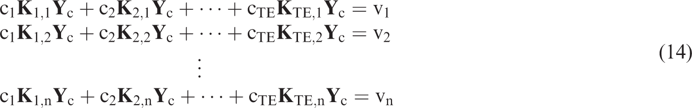
The system of equation above, which is strictly valid for a specific excitation frequency ω, can be solved simultaneously to obtain the extent coefficient of each element present in the structure. In order to solve all unknown extent coefficients, the amount of degrees-of-freedom in the structure must be equal to or greater than the number of elements present in the structure. However, this is not always the case. To tackle this problem, several sets of equations may be generated using different excitation frequencies $({\omega }_{\text{1}},{\omega }_{\text{2}},\mathrm{\dots },{\omega }_{\text{e}})$ , where the subscript $\text{e}$ represents the amount of excitation frequency used. Following this approach, a new set of equations can be formed by selecting $\text{TE}$ equations from the generated sets of equations, followed by solving the new set of equations simultaneously to obtain the extent coefficients.

Stage 2: Removal of temperature effect for damage coefficient assignment

After each element has been assigned with an extent coefficient, the temperature effect should be removed to give the damage locations and extent of the damaged elements. The extent coefficient ${\text{c}}_{\text{s}}$ obtained for each element after the application of equation (14) can be decomposed into its contributing factors, which are the temperature effect and the damage effect as follows

$${\text{c}}_{\text{s}}={\text{c}}_{\text{t,s}}+{\text{c}}_{\text{d,s}}$$

(15)

where

${\text{c}}_{\text{t,s}}$ is a temperature coefficient representing the percentage reduction/increase in elemental stiffness of the $\text{sth}$ element due to the effect of the changing temperature from the reference baseline temperature used to calculate the extent coefficient ${\text{c}}_{\text{s}}$ ;

${\text{c}}_{\text{d,s}}$ is a temporary damage coefficient representing the percentage reduction in elemental stiffness of the $\text{sth}$ element from the stiffness obtained at reference temperature used to calculate the extent coefficient ${\text{c}}_{\text{s}}$ due to the effect of damage.

The coefficient ${\text{c}}_{\text{d,s}}$ is temporary because the amount of reduction in stiffness used to calculate the percentage is compared to the stiffness obtained at reference temperature; however, since the temperature of the structure being monitored has changed, to know the actual percentage reduction in stiffness, this amount of reduction should be compared to the stiffness at the current temperature condition (without the effect of damage), and not to the stiffness obtained at the reference temperature condition. This is because, for the same amount of percentage reduction in stiffness, different temperature condition will have different amount of reduction in stiffness. Thus, a new damage coefficient, ${\text{D}}_{\text{s}}$ , needs to be defined and assigned to the elements to get the actual percentage reduction in elemental stiffness due to damage effect. To be able to obtain the damage coefficients of the elements to represent the percentage reduction in stiffness due to damage, the temperature coefficient of each damaged element needs to be estimated first so that the stiffness of the element at its current temperature condition (without the effect of damage) can be obtained and be used for comparison. This can be achieved by using the temperature coefficients of the undamaged elements to estimate the temperature coefficients of the damaged elements. Thus, the temperature coefficient of the $\text{sth}$ element may be obtained as follows

$${\text{c}}_{\text{t,s}}={\text{g}}_{\text{1}}+{\text{g}}_{\text{2}}{\text{L}}_{\text{s}}+{\text{g}}_{\text{3}}{\text{L}}_{\text{s}}^2$$

(16)

where

${\text{g}}_{\text{1}},{\text{g}}_{\text{2}}$ , and ${\text{g}}_{\text{3}}$ are undetermined coefficients;

${\text{L}}_{\text{s}}$ is the distance between the $\text{sth}$ element and a preset reference zero coordinate system.

Equation (16) is a quadratic equation representing the variation of the Young’s modulus across the structure from the initial Young’s modulus used as reference and obtained at the reference temperature, due to the gradient temperature across the structure and to the nonlinear effect of the changing temperature condition on the vibration properties and frequency responses of the structure. Equation (16) is in the form of a quadratic equation so as to take into account nonlinear gradient of temperature across the structure as well as nonlinear effect produced by temperature condition. Equation (16) can be obtained by first plotting the extent coefficients of the all the elements, followed by finding the equation of the line joining all the extent coefficient values together. However, it should be noted that the damaged elements should have their damage effects contribution to the extent coefficients removed before creating the equation of the line. To do this, the graph of the extent coefficients of all the elements versus the elements’ number (ranked in order with the distance between them) should first be plotted. Then, examining the graph, the damage locations can be obtained by the appearance of peaks in the graph. These peaks represent the contribution of damage to the extent coefficients. Thus, by eliminating the peaks in the graph, the equation of the line can then be generated. The values of the coefficients ${\text{g}}_{\text{1}},{\text{g}}_{\text{2}}$ , and ${\text{g}}_{\text{3}}$ can thus be obtained by defining the line. Substituting any value of ${\text{L}}_{\text{s}}$ in the equation which represents the distance of the $\text{sth}$ element to the reference zero coordinate, the temperature coefficient for that element can then be estimated. It should be noted that a lower/higher order polynomial function can be adopted to best represent the extent coefficient profile.

To give the percentage reduction of elemental stiffness of the $\text{sth}$ element due to damage, a damage coefficient ${\text{D}}_{\text{s}}$ may be defined. This damage coefficient compares the amount of reduction in stiffness due to damage of each element to the actual stiffness of the element due to temperature effect only. The damage coefficient ${\text{D}}_{\text{s}}$ can be related to the temporary damage coefficient ${\text{c}}_{\text{d,s}}$ as follows

$${\text{D}}_{\text{s}}\equiv \frac{{\text{c}}_{\text{d,s}}}{1-{\text{c}}_{\text{t,s}}}$$

(17)

where

${\text{D}}_{\text{s}}$ is the damage coefficient of the $\text{sth}$ element;

$(1-{\text{c}}_{\text{t,s}})$ represents the elemental stiffness of the $\text{sth}$ element at its current temperature condition without the effect of damage, in terms of a percentage of the stiffness obtained at the reference temperature used to calculate the extent coefficient.

Substituting equations (16) and (17) into equation (15) leads to

$${\text{c}}_{\text{s}}=({\text{g}}_{\text{1}}+{\text{g}}_{\text{2}}{\text{L}}_{\text{s}}+{\text{g}}_{\text{3}}{\text{L}}_{\text{s}}^2)+{\text{D}}_{\text{s}}(1-({\text{g}}_{\text{1}}+{\text{g}}_{\text{2}}{\text{L}}_{\text{s}}+{\text{g}}_{\text{3}}{\text{L}}_{\text{s}}^2))$$

(18)

Rearranging equation (18), the damage coefficient ${\text{D}}_{\text{s}}$ for each element can be obtained as

$${\text{D}}_{\text{s}}=\frac{{\text{c}}_{\text{s}}-({\text{g}}_{\text{1}}+{\text{g}}_{\text{2}}{\text{L}}_{\text{s}}+{\text{g}}_{\text{3}}{\text{L}}_{\text{s}}^2)}{1-({\text{g}}_{\text{1}}+{\text{g}}_{\text{2}}{\text{L}}_{\text{s}}+{\text{g}}_{\text{3}}{\text{L}}_{\text{s}}^2)}$$

(19)

From equation (19), the damage coefficient, ${\text{D}}_{\text{s}}$ , for the $\text{sth}$ element can be obtained. Undamaged element will have ${\text{D}}_{\text{s}}$ value of zero, while damaged element will have ${\text{D}}_{\text{s}}$ value ranging from zero to one, with one representing fully damaged. It should be noted that this way of calculating ${\text{c}}_{\text{t,s}}$ for each element allows the proposed method to perform for structures, which have nonlinear temperature gradient across the structure as well as structures whose vibration properties and frequency responses are affected nonlinearly by the changing temperature condition.

Summary of the method

Below are the procedures to follow to implement the proposed damaged detection method, and Figure 1 summarizes the procedures in the form of a flowchart.

Apply a harmonic excitation force to the structure in its undamaged state to gather frequency responses of the structure for the baseline of the undamaged structure.

If there are more elements than the number of degrees-of-freedom available, several harmonic excitation forces with different excitation frequencies should be applied to the structure one at a time.

The temperature condition along the structure can have a nonlinear profile which is usually the case for real-life structures.

Apply the same harmonic excitation force(s) to the structure when monitoring is required to gather new frequency responses of the structure.

 • It does not matter whether the temperature is constant or has a gradient distribution throughout the structure.

Use the frequency responses obtained from steps 1 and 2, and apply equation (14) to obtain the extent coefficient ${\text{c}}_{\text{s}}$ of each element.

Plot the extent coefficients obtained against the elements’ number and analyze the graph to locate the damaged elements.

 • The damaged elements will appear as peaks in the plot.

Use extent coefficients from all the undamaged and damaged elements (ignoring the contribution of the damage effect to the extent coefficient) for the creation of the equation of the line (temperature effect trend) in the form of equation (16) so that the temperature coefficient ${\text{c}}_{\text{t,s}}$ of each element can be calculated.

 • Equation (16) is in the form of a quadratic equation; however, a lower/higher order polynomial function can be used to best represent the trend of the temperature condition.

Apply equation (19) to obtain the damage coefficient ${\text{D}}_{\text{s}}$ of each element to get the damage locations and extent.

 • The undamaged elements will have damage coefficient of zero, while the damaged elements will have damage coefficient ranging from zero to one, with one representing fully damaged.

Figure 1.

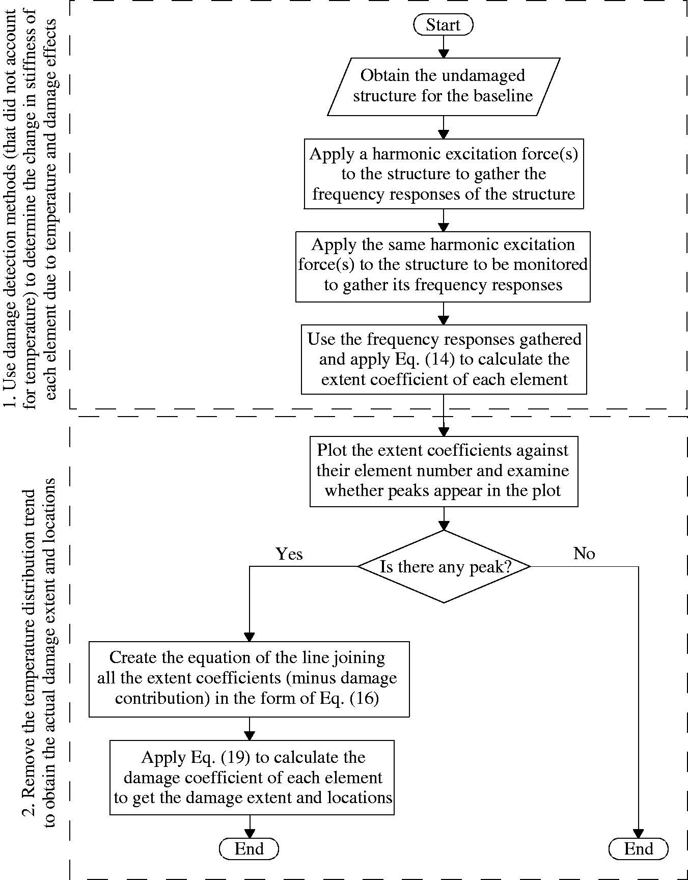
Flowchart of the procedures to follow for damage detection.

It is worth noting that stage 2 of the method can be implemented with other damage detection methods that did not account for temperature effect to eliminate the influence of varying temperature condition and allow the locations and extent of damages to be obtained, while the damage detection method proposed in stage 1 can be replaced by other damage detection methods that can give the amount of change of stiffness due to external factors from a baseline stiffness. To this end, the procedures given above can be modified accordingly; the first three steps in the procedure can be replaced by other damage detection methods, while the last three steps can be incorporated in the selected damage detection method to eliminate the temperature effect and to locate and quantify damages.

Numerical examples

To demonstrate the proposed approach for damage detection, localization, and quantification, a beam structure representing a model bridge and a shear building are used as case studies. The two structures are adopted since it is well known that temperature condition along long span bridges and tall buildings usually varies, hence, influencing the dynamic properties of the structures.

Beam structure

The beam structure used for demonstration is shown in Figure 2. It is 15-m long, with one end (end A) being pin connected and the other end (end B) being free. At 10 m from the pin-connected end, the structure rests on a roller support. The structure is assumed to be made of steel material with a Young’s modulus of 200 GPa and density of 7850 $\text{kg}/{\text{m}}^3$ . The cross-sectional area and the second moment of area of the beam are assumed to be 0.08 ${\text{m}}^2$ and 0.0006 ${\text{m}}^4$ , respectively. The two-dimensional numerical model of the structure is built in MATLAB and it is discretized into 15 beam elements of 1-m long each. A harmonic excitation force with ω = 2000 rads/s is applied at the free end (B) pointing downward to generate the frequency responses of the structure.

Figure 2.

Two-dimensional beam structure.

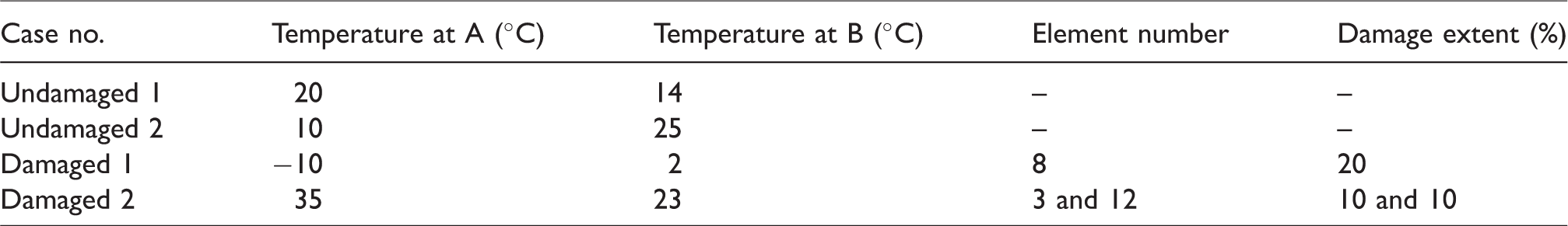
To simulate the effect of varying temperature condition, the Young’s modulus of the steel material is assumed to be temperature dependent as suggested by An et al. ²⁴ Since it was found in the literature that temperature condition usually has nonlinear relationship with the vibration properties of civil engineering structures,^25,26 the hypothetical variation of Young’s modulus with temperature is assumed to be nonlinear as can be seen in Figure 3. To consider the effect of temperature gradient across the structure, two undamaged cases and two damaged cases are used to demonstrate the proposed approach, and the descriptions of the cases are presented in Table 1. Figure 4 illustrates the temperature variation across the beam structure. In this beam structure, damage is assumed to be represented by a reduction in elemental stiffness of the structural components.

Figure 3.

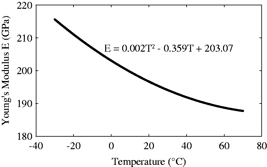
Hypothetical variation of Young’s modulus with temperature.

Table 1.

Descriptions of undamaged and damaged cases subjected to nonlinear temperature gradient across the structure.

Case no.	Temperature at A (°C)	Temperature at B (°C)	Element number	Damage extent (%)
Undamaged 1	20	14	–	–
Undamaged 2	10	25	–	–
Damaged 1	−10	2	8	20
Damaged 2	35	23	3 and 12	10 and 10

Figure 4.

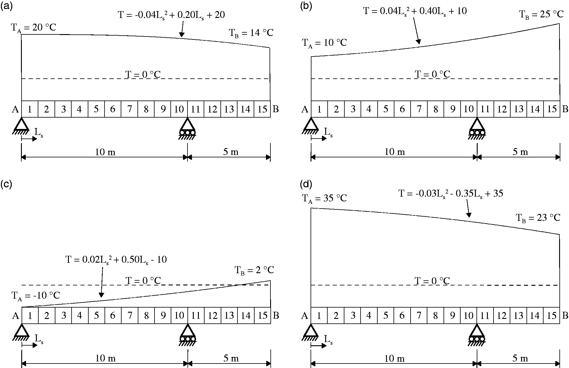
Temperature variation across the beam structure for (a) undamaged case 1, (b) undamaged case 2, (c) damaged case 1, and (d) damaged case 2.

Since generally structures are faced with gradient temperature, a nonlinear temperature distribution is assumed for the baseline of the undamaged structure. The temperature condition of the baseline of the undamaged structure from which subsequent measurements can be compared with is given in Figure 5. Note that any temperature could have been used as baseline. After applying the proposed damage detection method, and the application of equation (14), the extent coefficient ${\text{c}}_{\text{s}}$ of each element for each case can be obtained. Since generally noise affects the performance of damage detection methods, to demonstrate the robustness of the second stage of the proposed approach to eliminate the effect of temperature conditions to give the damage locations and extent, 10% of noise is added to the extent coefficients. The performance of the approach of eliminating the effect of temperature is dependent upon the extent coefficients, which in turn are dependent upon the techniques used to obtain these coefficients in stage 1. Therefore, it is the extent coefficients that are polluted with noise, to demonstrate that the proposed approach can still be applied for cases where the extent coefficients are subjected to errors. The polluted extent coefficients are given by

$${\widehat{\text{c}}}_{\text{s}}={\text{c}}_{\text{s}}(1+\frac{\aleph }{100}\Re )$$

(20)

where

Figure 5.

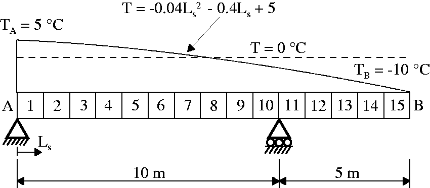
Temperature variation across the undamaged beam structure used as baseline.

${\widehat{\text{c}}}_{\text{s}}$ is the polluted extent coefficient;

$\aleph$ is the specified noise level added to the extent coefficients and taken as 10 in this case study;

$\Re$ is a random number between −1 and 1.

Plots of the extent coefficients (polluted with noise) for the four cases under consideration are presented in Figure 6. It can be seen from Figure 6(a) and (b) that for the undamaged cases, no damage is present in the structure, since no consequent peak appears in the plots. Some fluctuations in the first plot can be seen in the middle portion of the beam; however, no obvious peak that indicates an abrupt and large change in stiffness exists. Figure 6(c) and (d) give the plots of the two damaged cases. It can be seen from both plots that peaks appear to alert the presence of damages in the structure. The first damaged case (Figure 6(c)) has a peak at element 8, which indicates that element 8 is damaged, while the second damaged case (Figure 6(d)) has two peaks at elements 3 and 12, respectively, suggesting that these two elements are damaged. By constructing equation (16) to determine the temperature coefficient of each element, and by applying equation (19), a damage extent of 20% for element 8 can be calculated for the first damaged case, while for the second damaged case, elements 3 and 12 are found to have a reduction in elemental stiffness of 10% and 11%, respectively.

Figure 6.

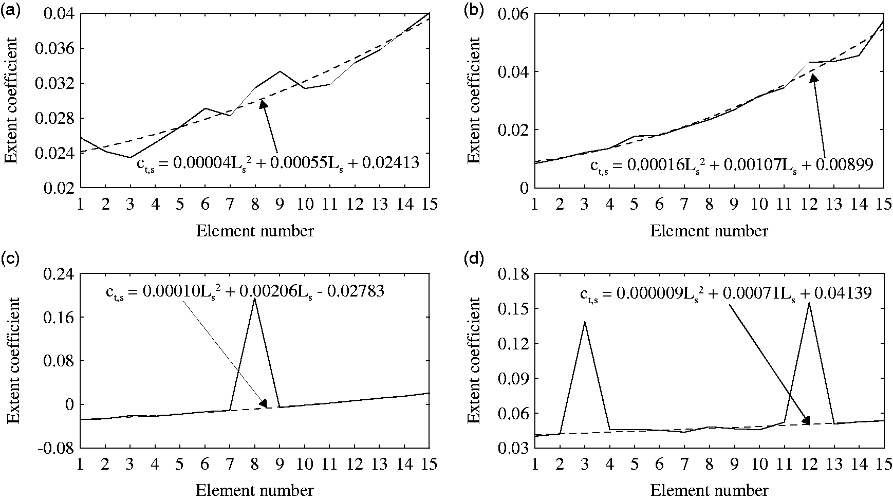
Extent coefficient plot of beam structure for (a) undamaged case 1, (b) undamaged case 2, (c) damaged case 1, and (d) damaged case 2.

From the four plots shown in Figure 6, it can also be seen that the extent coefficient values of the undamaged elements generally vary smoothly from element to element throughout the structure. This can be attributed to the fact that, for the undamaged element, the amount of change in stiffness is due fully to the deviation in temperature from the baseline temperature condition, and since temperature condition along a structure usually changes gradually from location to location, the change of stiffness of each element, which is represented by the extent coefficient, will increase/decrease steadily along the structure. Only a significant variation in the amount of change in stiffness from an element to the nearby elements will produce a sharp change in the extent coefficient profile. As damage is a localized effect which produces a significant decrease in stiffness of the damaged element, it will produce a sudden change in the extent coefficient plot. Thus, any sharp change/peak in the plot can be attributed to the effect of damage. Noise affecting the measurements will also create a change in the extent coefficient plot, however, these fluctuations will be much less when compared to the effect of damage and no distinct peak will occur. Peaks at the damage locations will always exist because the extent coefficient combines the amount of change of stiffness due to temperature and damage effects together. It can therefore be concluded that for a damaged element, the temperature contribution to the extent coefficient will follow the same trend as other undamaged elements’ extent coefficients, while the contribution of damage will be an addition to that trend. By observing the extent coefficient plot, the temperature and damage effects can be distinguished, and the damage extent can be quantified through the peaks’ contribution.

Shear building

A shear building (Figure 7(a)) is also used as another example to demonstrate the applicability of the proposed approach for damage localization and quantification, since buildings’ vibration properties are commonly affected by the changing temperature condition they are faced with.^27,28 The numerical model of the shear building is the same as the one used as case study by Roy and Ray-Chaudhuri. ²⁹ The shear building is 12-story high with uniform story mass and stiffness distribution throughout the height of the structure. The story mass and stiffness properties adopted in this paper are $1\times {10}^5$ kg and $2\times {10}^8$ ${\text{Nm}}^{\text{-1}}$ defined at reference temperature of 20°C, respectively. A harmonic excitation force with angular frequency ω = 1000 rads/s is applied at the first floor level to generate the frequency responses of the structure.

Figure 7.

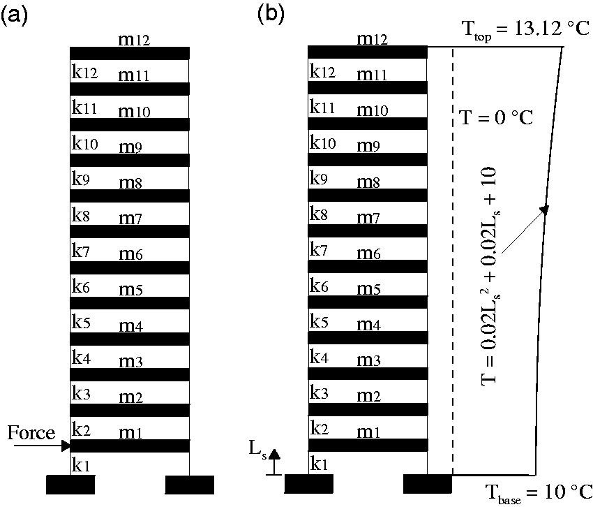
(a) Two-dimensional shear building structure and (b) temperature variation across the undamaged shear building used as baseline.

To simulate a varying temperature condition, it is assumed that the stiffness of the structure varies nonlinearly with the temperature condition. The relationship between the temperature condition and the story level stiffness is given by equation (21). The story stiffness is assumed to vary nonlinearly with the temperature condition because Young’s modulus of structures generally varies with a changing temperature condition, which as a result, affects the stiffness of the structures. The temperature distribution across the undamaged structure used as baseline is given in Figure 7(b). Damage is simulated as a reduction in story-level stiffness, and the scenarios applied to the shear building are presented in Table 2. The temperature profile along the structure for the different cases are shown in Figure 8, and it is assumed that the temperature condition at the top of the building is greater than that at the bottom since buildings are subjected to greater radiation at their roof level than at their base level. Similar to the beam case study, 10% of noise is added in this shear building case study.

$${\text{k}}_{\text{s,t}}=1.2\times {10}^4{\text{T}}^2-9.2\times {10}^5\text{T}+2.136\times {10}^8$$

(21)

where

Table 2.

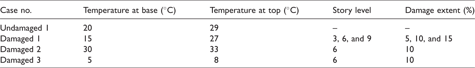
Descriptions of undamaged and damaged cases subjected to nonlinear temperature gradient throughout the shear building.

Case no.	Temperature at base (°C)	Temperature at top (°C)	Story level	Damage extent (%)
Undamaged 1	20	29	–	–
Damaged 1	15	27	3, 6, and 9	5, 10, and 15
Damaged 2	30	33	6	10
Damaged 3	5	8	6	10

Figure 8.

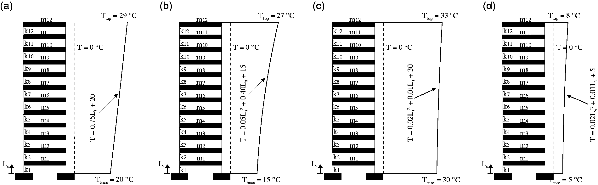
Temperature variation throughout the shear building structure for (a) undamaged case 1, (b) damaged case 1, (c) damaged case 2, and (d) damaged case 3.

${\text{k}}_{\text{s,t}}$ is the stiffness of the sth story considering temperature effect in $\mathrm{N}{\mathrm{m}}^{-1}$ ;

$\text{T}$ is the temperature condition of the sth story in °C.

The plots of the extent coefficients versus story’s level for the four cases are presented in Figure 9. It can be seen from Figure 9 that the cases are well classified; the first plot (Figure 9(a)) indicates no damage is present, while the following three plots ((Figure 9(b)–(d)) show that the structure is damaged due to the appearance of peaks. It can again be seen that the temperature effect produces a relatively smooth change of extent coefficient from undamaged story to undamaged story, while damage effect produces a sharp change in extent coefficient of the damaged story from the nearby stories. This sharp change in extent coefficient represents the extra contribution in decreasing the stiffness of the damaged story. Applying equation (19), it is found that the first damaged case has story levels 3, 6, and 9 to have a reduction in stiffness by 5%, 10%, and 16%, respectively, the second damaged case has 9% reduction in the sixth story, while the last case has a reduction in stiffness of 10% in the sixth story.

Figure 9.

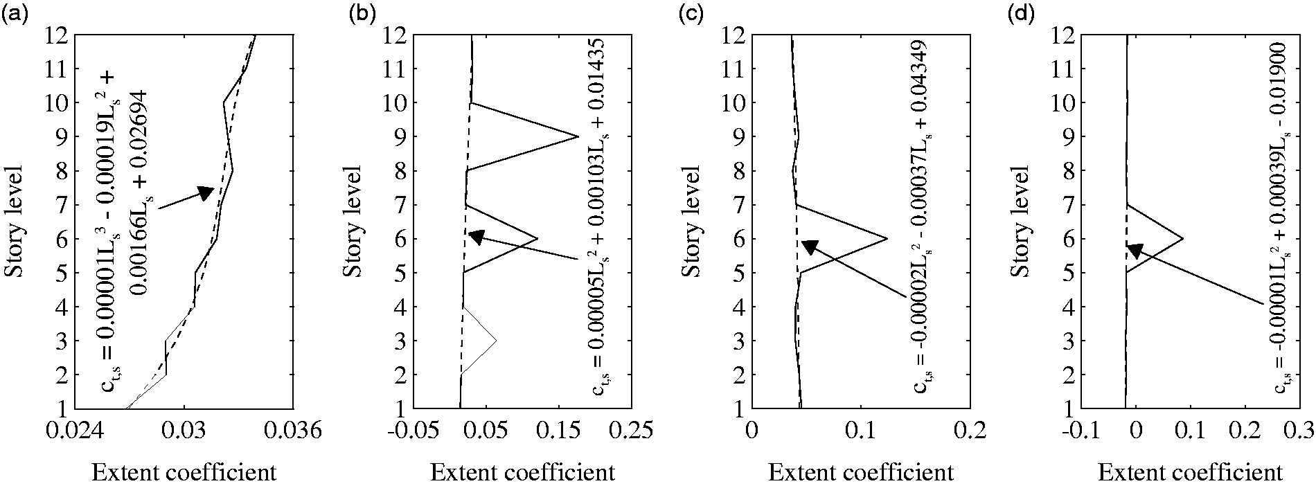
Extent coefficient plot of shear building for (a) undamaged case 1, (b) damaged case 1, (c) damaged case 2, and (d) damaged case 3.

For this damage detection method, the temperature trend can be found through the quadratic function given by equation (16). For example, from Figure 9(a), it can be seen that the first undamaged case has a nonlinear change in extent coefficient. This case is analyzed in this paper to demonstrate that, depending on the profile of extent coefficient, the function given through equation (16) can be adjusted to suit the extent coefficient profile. Being able to adjust the function order allows the proposed approach to closely represent the temperature coefficient of each element, thus decreasing the chance of obtaining the wrong damage scenario. For example, for the first undamaged case (Figure 9(a)), a cubic function is adopted; therefore, a cubic part is added to the quadratic function (equation (16)).

One potential difficulty of the proposed approach is how to quantify the extent of damages through the peaks, since different temperature condition will produce different peak contributions. For instance, the last two damaged cases have the same damaged element with the same damaged extent, but with different temperature condition. Quantifying the peak amount by subtracting the temperature coefficient of that element from its extent coefficient, it is found that the second damaged case (Figure 9(c)) has a value of 0.083, while the third damaged case (Figure 9(d)) has a value of 0.104. The difference in these two values is attributed to the different temperature conditions the two cases are at, since different temperature condition will produce different amount of change of stiffness for the same percentage of reduction in stiffness. This issue can be overcome by deriving relationships between the change in stiffness due to damage, and the stiffness of the elements at the current temperature condition. For example, for the proposed damage detection method, the damaged elements can be quantified through equation (19), which relates the peak contribution to the stiffness of the members at the current temperature condition.

Discussion of the proposed approach

The principle behind most conventional damage detection methods that did not take into account temperature effect is to compare new measurements to a single benchmark so as to determine which member has a change in stiffness from the original elemental stiffness, and to quantify this change for damage localization and quantification. Since damage is the only effect considered in the methods that will cause change in stiffness, only the damaged elements will have a reduction in stiffness, however, most civil engineering structures are subjected to changing temperature condition, and both damage and temperature effects will change the stiffness of the elements. Therefore, obtaining the total change in stiffness due to both damage and temperature effects first, followed by removing the temperature effect, will facilitate damage localization and quantification.

In the aspect of creating a baseline for damage detection, most approaches have difficulty in creating a baseline when encountering temperature gradient along the structures, which generally has a great influence on the vibration properties. This condition is commonly found when analyzing long span bridges and tall buildings because ambient solar radiations are not evenly distributed along the structures. Limited methods were proposed in the literature to tackle gradient temperature condition along the structures for damage localization and quantification. The reason behind may be attributed to the difficulty in creating a baseline of the undamaged structure which is commonly constructed using a wide range of temperature conditions, to include all possible conditions the structure may encounter, since there is an infinite amount of temperature profiles that the structure can be faced with. Moreover, gradient temperature may overestimate/underestimate temperature effect on the vibration properties, if the temperature profile is not accounted for properly, hence leading to false alerts.

To tackle this gradient temperature and temperature condition issue in general, drawing the extent coefficient profile of the structure due to temperature effect, seems to be the best solution since no predefined solution for that profile is required to be included in the baseline, and this extent coefficient profile can be obtained using the global trend of change in stiffness. To this end, this paper uses a quadratic function to represent the global change in elemental stiffness which can then be related to the temperature distribution along the structure. It is important to allow the profile of extent coefficient to be represented by a quadratic function or even higher order polynomial function because, if the profile can only be represented by a linear function, the temperature coefficient would be underestimated/overestimated, hence underestimating/overestimating the contribution of temperature in changing the stiffness of the elements, leading to false damage extent and locations. It should be noted that the quadratic function defining the temperature distribution profile along the structure (e.g., Figure 4) is different from the one describing the profile of extent coefficient (e.g., Figure 6). This difference is attributed to the nonlinear relationship between the Young’s modulus of the material and the temperature as well as the temperature profile of the baseline structure, which were accounted for by the extent coefficient plot, and not by the temperature distribution profile along the structure.

Using only one reference temperature as baseline is proposed in this paper, as it has the advantage that the damage detection method can give the damage locations and extent since the structure can be compared locally to the baseline. Moreover, the method can be implemented immediately without requiring months of measurements to create the baseline of the undamaged structure. It also reduces the risk of false alerts which may occur for structures that have temperature–Young’s modulus relationship to be nonlinear, since, if not all conditions are included in the baseline, false alerts may occur. The proposed approach eliminates the risk that small damages are not detected, which may occur if a range of temperature condition is used, because the small damages may not alter the dynamic properties significantly enough to trigger the damage alert. Therefore, by using the proposed approach, the difficulty of using a range of temperature condition for the baseline of the undamaged structure for damage localization and quantification is enhanced, as it can easily tackle any temperature profile along the structure. This approach is appealing because it can be incorporated in most existing damage detection methods easily by first using the damage detection methods to quantify the changes in stiffness of all the elements due to temperature and damage effects, followed by removing the temperature contribution which is a global effect by finding the temperature trend, to obtain the damage locations and extent.

Conclusion

A new insight on how to approach damage detection of civil engineering structures subjected to varying temperature and to gradient temperature conditions by using a single temperature profile as the baseline is introduced in this paper. The approach uses the concept of first quantifying the change in stiffness of all the elements due to the effects of temperature and damage, and then the temperature effect which has a global trend on the structure is removed, to give the damage locations and extent. The approach is implemented with a proposed damage detection method that did not account for temperature effect, to be able to tackle varying temperature and gradient temperature conditions. The damage detection method with the proposed approach incorporated is tested for different undamaged and damaged cases using a beam structure and a shear building subjected to gradient temperature conditions. The results demonstrate that, by quantifying the change in stiffness of all the elements due to external factors, the trend of temperature effect along the structure can be obtained, as well as the damage locations. This temperature effect is found to be different from the damage effect, which is a localized effect, thus, the actual damage locations and extent can be obtained by eliminating the temperature effect. The proposed approach can be implemented with other damage detection methods that did not account for temperature effect to obtain the damage locations and extent under changing temperature condition.