Acoustic impedance tuning with active disturbance rejection control

Abstract

An anechoic end is desired to be implemented on an acoustic test rig. The acoustic impedance can be tuned with active control, such as phase shift control. A precise mathematical description of a system is necessary for phase shift control. However, in some cases, the mathematical model is inaccurate and even impossible to obtain. To overcome the weakness, active disturbance rejection control is proposed as a model-independent strategy and is tested on an identified model and test rig for comparison to phase shift control. The results of the simulation and the experiment show that the performance of phase shift control is strongly influenced by the accuracy of the model, and active disturbance rejection control achieved good performance in the absence of a proper model. Furthermore, a Lyapunov function is constructed to prove the asymptotic stability of active disturbance rejection control, thus ensuring the stability and robustness of the control system.

Introduction

In the field of noise control, low-frequency sound is very difficult to absorb via a passive control approach, because a large sound-absorbing structure is required. By contrast, active control is much more suitable for low-frequency noise control. Previously, active control was proposed in theory to reduce undesired sound by introducing secondary sound, which is designed to be nearly 180° out of phase with the sound from primary source.^1,2 Olson and May ³ proposed the earliest practical application of active control, which was called the electronic sound absorber; using this approach, the sound generated by primary source can be suppressed, and the sound pressure level can be reduced 10–25 dB. However, the controller was an analogue circuit, so the parameters of controller are difficult to be modified after the controller is designed. With the development of chip technology, the digital signal processor (DSP) becomes much more inexpensive and faster. As a result, active control based on DSP has drawn much attention and effort from researchers and engineers. In the last two years, there are many researches on active noise control (ANC), such as active noise equalizer, ⁴ reference frequency mismatch in ANC, ⁵ and ANC based on wavelet function and network approach. ⁶ Another approach to suppress noise is active vibration control (AVC), in which actuators are applied directly on the vibrating structures. Existing researches include AVC of variable section cylindrical structures, ⁷ natural frequency adjustable electromagnetic actuator, ⁸ ANC of conical shell, ⁹ and so on.

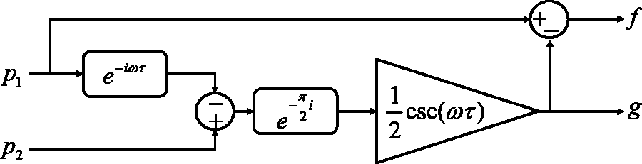
In addition to the aforementioned applications, active control is also applied to the acoustic impedance tuning. Acoustic impedance is defined as the ratio of pressure fluctuation and velocity fluctuation. According to acoustic theory, there is a relationship between the acoustic impedance and the reflection coefficient. There are many applications of acoustic impedance tuning; sometimes, a desired acoustic impedance condition, such as an anechoic end, is necessary to satisfy the requirements of some applications; Saurabh et al. ¹⁰ proposed the research of swirl flame response to travelling acoustic waves in 2014. As the reflections of acoustic waves in a duct are inevitable, the travelling wave mode is almost impossible in the state of nature. Thus, the acoustic impedance tuning approach is adapted to Saurabh’s work.

Until now, there are several investigations regarding the active control of the acoustic impedance in a duct. Guicking and Karcher ¹¹ proposed an active impedance control scheme for one-dimensional sound. Two pressure transducers are set at different positions to measure the local pressure signal, and travelling wave components are decomposed using the Two-Microphone Method (TwMM). The control scheme is based on phase shift control. The acoustic impedance can be tuned from nearly fully absorbing to fully reflecting. Bothien et al.^12–16 improved Guicking’s approach and proposed a type of active control scheme that is applicable for a combustion system. The loudspeakers are placed at the sidewall of duct to allow a mean flow to be added to the duct. The control scheme is also based on phase shift control. Li et al. ¹⁷ proposed a scheme of realizing a standing wave tube by acoustic impedance control. In their work, impedance matching is implemented by repetitive control. By tuning the phase difference and the amplitude ratio of two loudspeakers, different acoustic impedances can be achieved in theory.

Despite the prior achievements, some shortcomings remain in these previous works: the parameters of the controller in Guicking’s paper are tuned by hand, which is inconvenient for industrial applications; both phase shift control and repetitive control require a precise modelling of the system, as the model error would cause instabilities of the control system. However, for a real system, sometimes we cannot obtain enough information to model it, implying that model-based control scheme is not feasible for complicated or unknown systems. To extend the applications of active control of acoustic impedance, model-independent control scheme must be introduced, which is called active disturbance rejection control (ADRC).

ADRC was originally proposed by Han ¹⁸ in 1998 to solve the uncertainties in nonlinear systems. To simplify the design and parameters tuning, a linear ADRC and a bandwidth-parameterization method were proposed by Gao. ¹⁹ The theoretical proofs of ADRC demonstrated the convergence of ADRC ²⁰ and the stability of ADRC.^21,22 Linear ADRC inherits the easy use of a PID controller and can estimate and compensate the unmeasured disturbance and unmodelled dynamics by extended state observer (ESO). ²³ ADRC does not rely on the precise system modelling because of the ability to estimate and compensate the total disturbance in real time. ²⁴ Because of its ease of use and excellent control performance, ADRC has been successfully applied to many industrial occasions, such as motion control, ²⁵ chemical process control, ²⁶ DC–DC power converter control, ²⁷ power plant control, ²⁸ and organic Rankine cycle control. ²⁹ However, to the best of the authors’ knowledge, the application of ADRC in acoustic impedance tuning has not been reported.

In this paper, two control schemes are applied to the acoustic impedance control: phase shift control and ADRC. In the next section, a precise model of system is established. In ‘Control approach’ section, the basic principles and parameter tuning approaches of phase shift control and ADRC are introduced. Lyapunov’s second method is applied to analyse the asymptotic stability of the first-order ADRC. In the ‘Results and analysis’ section, the results of simulation and experiment are illustrated. The final section gives the conclusion and the outlook of further work.

System identification

Test rig and measurement techniques

The active control experiment was developed on an acoustic test rig (Figure 1), which consists of plexiglass square duct segments. Its section size is 90 mm × 90 mm and the wall thickness is 15 mm. To guarantee the one-dimensional mode, ³⁰ the frequency of the sound wave should satisfy equation (1)

$$f<\frac{c_0}{2a}$$

(1)

where c₀ denotes the sound speed and a denotes the length of the side of square section. Equation (1) implies that the frequency of sound wave should be no more than 1890 Hz. To achieve different boundary conditions, a honeycomb tube is fixed at downstream, which is filled with honeycomb core. Considering the convenience of fixing pressure transducers, there are several threaded holes along the duct. To measure the pressure signal precisely, G.R.A.S. 40PL type CCP free-field array microphone is applied to the experiment. Its frequency response range is between 50 and 20 kHz. The sensitivity at 250 Hz is 10 mV/Pa. According to the user manual, the amplitude of 40PL microphone remains constant over a wide range. At both ends of the duct, loudspeakers with the same characteristics are fixed symmetrically.

Figure 1.

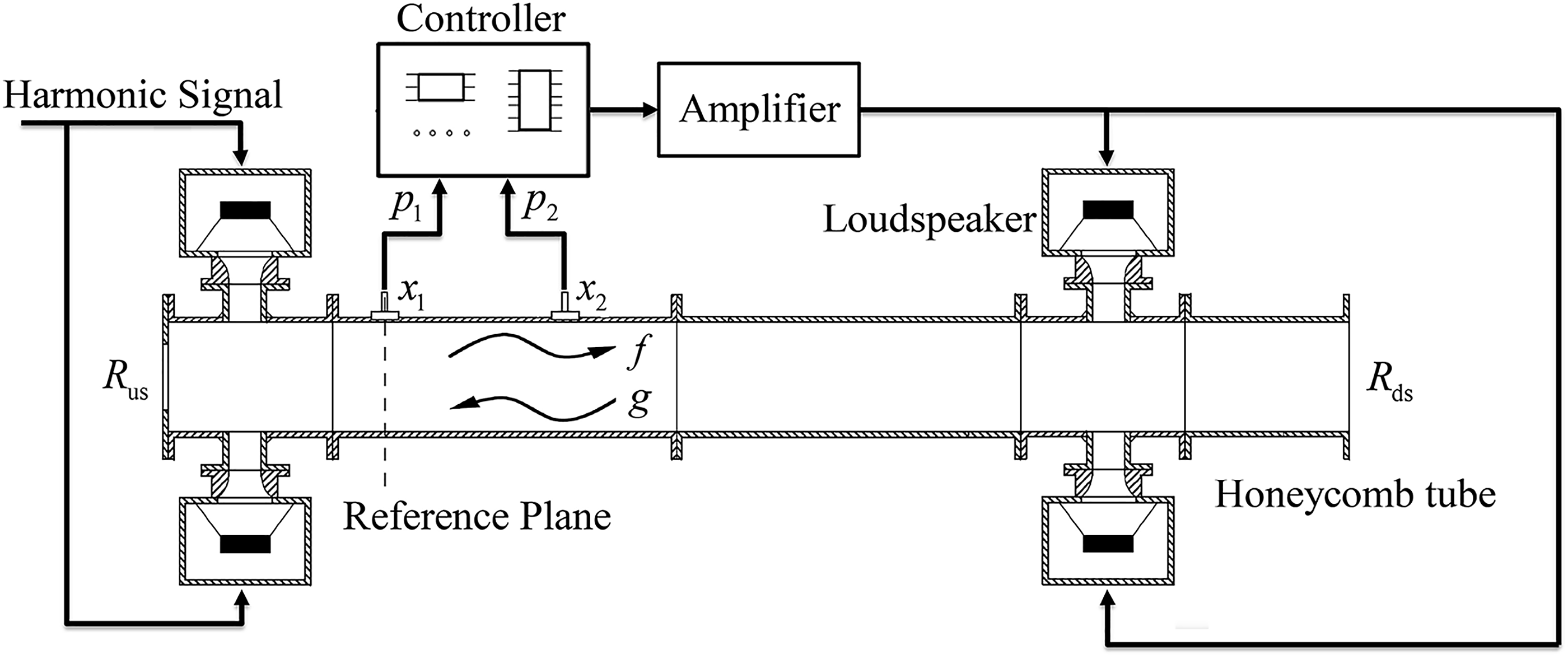
Schematic set-up of the active control test rig.

The loudspeaker used in the experiment is YD178-8X type woofer, which has an impedance value of 8 Ω and a power rating of 100 W (RMS). Its frequency response range is between 45 and 5000 Hz, and it has a sensitivity of 91 ± 3 dB.

TwMM

As mentioned in the last part, if the frequency of sound wave is lower than the cut-off frequency, which depends on the size of duct, then a one-dimensional sound field is formed. A one-dimensional sound field can be decomposed into travelling wave components: f-wave and g-wave. The reflection coefficient is defined as the ratio of g-wave to f-wave. The following is the relationship between the acoustic impedance and the reflection coefficient

$$\zeta =\frac{1+|R_{\text{ds}}|}{1-|R_{\text{ds}}|}$$

(2)

where ζ denotes the acoustic impedance, and R_ds denotes the downstream reflection coefficient. The measurement of the reflection coefficient is implemented using the TwMM, which is schematically shown in Figure 2.

Figure 2.

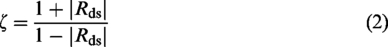
Block diagram of the TwMM.

TwMM can also be described in the form of equation (3)

$$\left[\begin{array}{l}f(\omega )\\ g(\omega )\end{array}\right]=\frac{1}{2i\sin (\omega \tau )}\left[\begin{array}{cc}{e}^{i\omega \tau }& -1\\ -e^{-i\omega \tau }& 1\end{array}\right]\left[\begin{array}{l}{p}_1(\omega )\\ p_2(\omega )\end{array}\right]$$

(3)

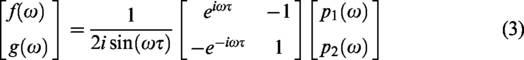
Taking advantage of TwMM, the f-wave and g-wave can be calculated online using a DSP; as a result, the active control of acoustic impedance is feasible.

Transfer function description of the test rig

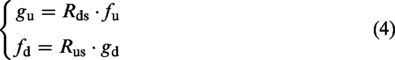
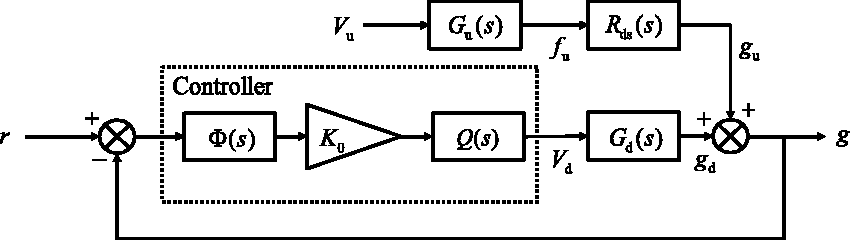
The whole test rig can be divided into upstream and downstream from the reference plane (Figure 3). The characteristic of the upstream loudspeakers is described by G_u(s), which implies the input–output relationship between the driving voltage V_u of the loudspeaker and the f-wave f_u at x₁; the characteristic of the downstream loudspeakers is described by G_d(s), which implies the input–output relationship between the driving voltage V_d of the loudspeaker and the g-wave g_d at x₁. Both g_u and f_d are generated by reflections, as described by equation (4)

$$\{\begin{array}{c}{g}_{\text{u}}=R_{\text{ds}}\cdot f_{\text{u}}\\ f_{\text{d}}=R_{\text{us}}\cdot g_{\text{d}}\end{array}$$

(4)

Figure 3.

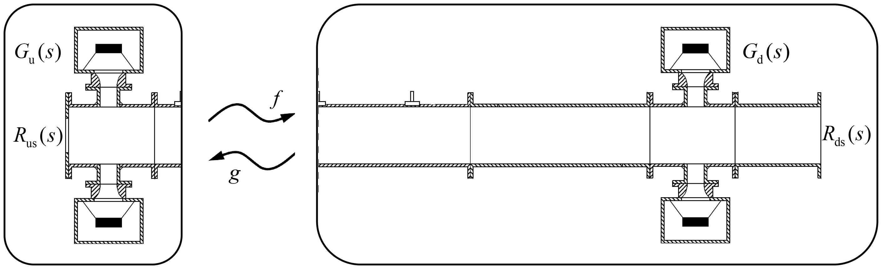
Schematic of a model describing the acoustic properties of the test rig.

Thus, the mathematical expressions of G_u(s), G_d(s), R_us(s), and R_ds(s) are to be identified. Weng et al. ³¹ proposed a model to describe the response of a loudspeaker. Here, a more precise model is proposed to describe G_u(s) and G_d(s). The model has a mathematical form given by equation (5)

$$G(s)=\left({\displaystyle \prod _{i=1}^m\frac{{\omega }_i}{s+{\omega }_i}}\right)\cdot \left({\displaystyle \sum _{j=1}^n\frac{A_{j}s+B_j{\omega }_j}{s^2+{\zeta }_{j}s+{\omega }_j^2}}\right)\cdot e^{-\tau s}$$

(5)

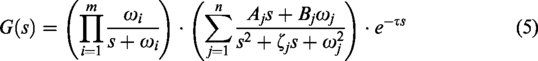
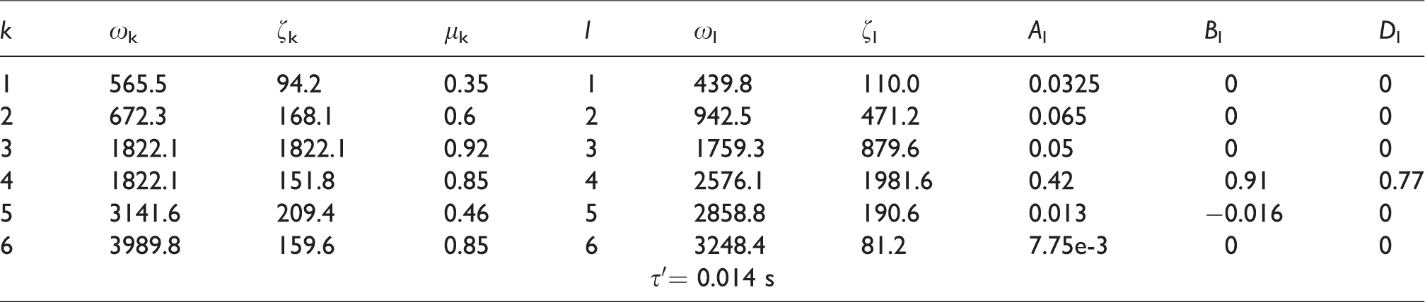
Equation (5) can be considered as a combination of three parts: low-pass filters, resonators, and time delay, where ω_i denotes the cut-off frequency of the low-pass filter, which is applied to guarantee the attenuation at high frequency; ω_j denotes the resonance frequency of the resonator; A_j and B_j are weight coefficients; τ denotes the acoustic propagation time in the duct and depends on the distance between loudspeakers and x₁. G_d(s) is a key to phase shift control. In other words, the more accurate the model is, the better the performance is. The modelling results are shown in Table 1 and Figure 4.

Table 1.

The parameters of G_u(s) and G_d(s).

Gu(s)					Gd(s)
i	ω i				i	ω i
1	2073.5				1	3518.6
2	3455.8				2	4209.7
3	4398.2				3	4398.2
j	ω j	A j	B j	ζ j	j	ω j	A j	B j	ζ j
1	439.8	64.4	0	280	1	565.5	40	0	160
2	879.6	50.4	0	105	2	911.1	40.5	0	90
3	1256.6	48.0	0	100	3	1288.1	27	0	90
4	1558.2	37.3	37.3	110	4	1633.6	23.2	0	80
5	1885.0	27.2	27.2	70	5	1947.8	33	0	60
6	2261.9	0	20	80	6	2324.8	35.4	35.4	100
7	2953.1	72.7	42	70	7	2638.9	45.0	26	130
8	3279.8	0	103.4	110	8	2953.1	0	72	60
9	3581.4	0	100	100	9	3298.7	0	83.6	190
10	3883.0	90	0	90	10	3644.2	0	76	190
11	4209.7	25.5	25.5	90	11	3958.4	0	26.4	110
12	4492.5	10.6	10.6	90	12	4335.4	0	13.5	90
τ = 0.0013 s					τ = 0.0060 s

Figure 4.

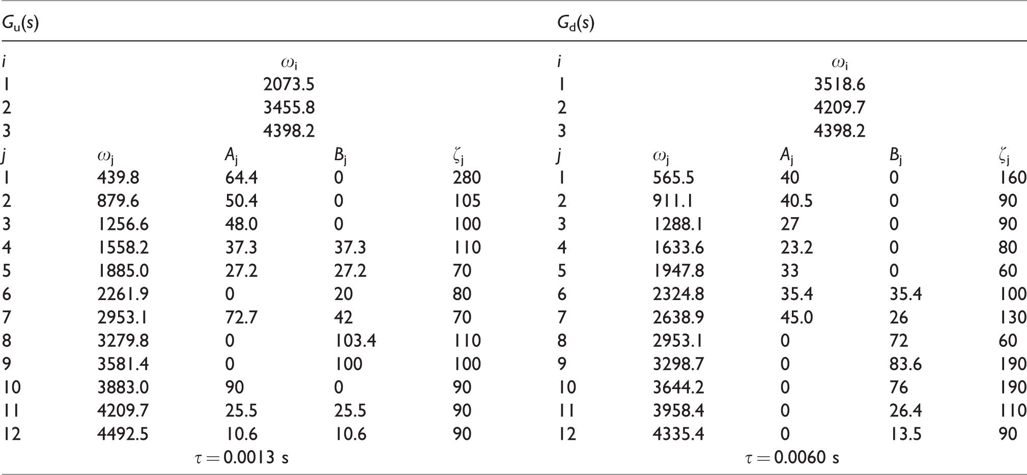
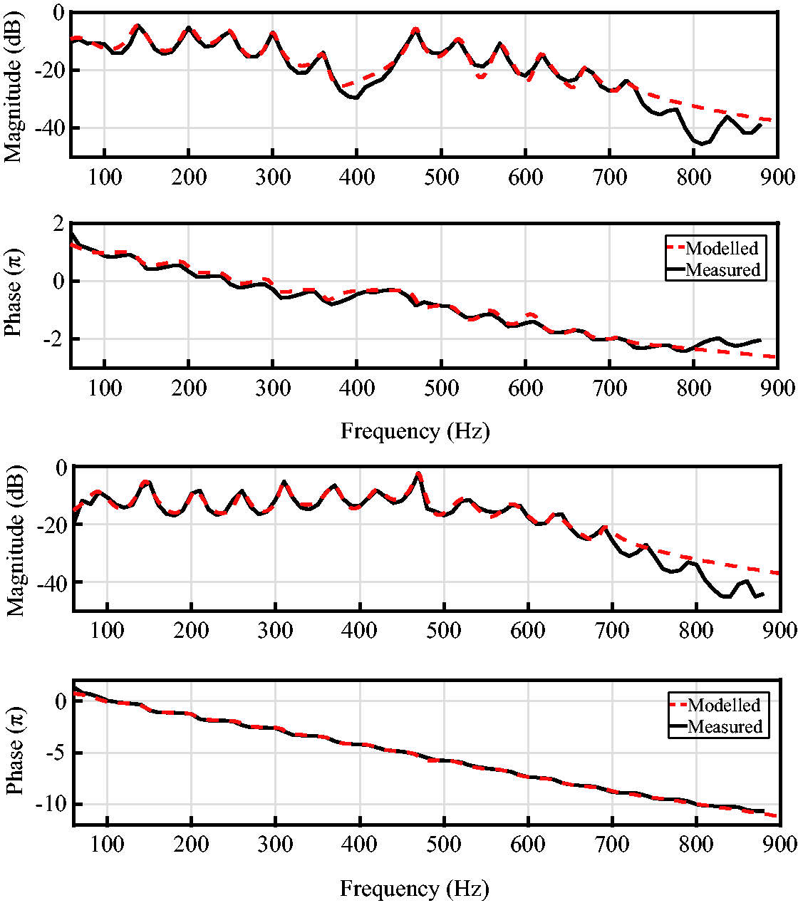
The best modelling of G_u(s) (top) and G_d(s) (bottom): m = 3, n = 12, 27th order.

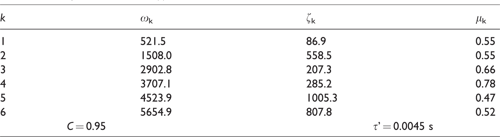
The models of R_us(s) and R_ds(s) are also desired. The upstream boundary is an open boundary. Here, the mathematical form of R_us(s) consists of two parts: bandstop filters and time delay, which is given by equation (6)

$$R_{\text{us}}(s)=C\cdot \left({\displaystyle \prod _{k=1}^h\frac{s^2+{\mu }_k{\zeta }_{k}s+{\omega }_k^2}{s^2+{\zeta }_{k}s+{\omega }_k^2}}\right)\cdot e^{-{\tau }^{\prime }s}$$

(6)

where μ _k  < 1 describes the absorption of acoustic wave at a certain frequency. As mentioned in ‘Test rig and measurement techniques’ section, there is a tube filled with honeycomb core fixed at downstream end. So we have to use a more complex model to describe R_ds(s), which is given by equation (7)

$$R_{\text{ds}}(s)=\left({\displaystyle \prod _{k=1}^h\frac{s^2+{\mu }_k{\zeta }_{k}s+{\omega }_k^2}{s^2+{\zeta }_{k}s+{\omega }_k^2}}\right)\cdot \left({\displaystyle \sum _{l=1}^r\frac{D_l{s}^2+A_l{\omega }_{l}s+B_l{\omega }_l^2}{s^2+{\zeta }_{l}s+{\omega }_l^2}}\right)\cdot e^{-{\tau }^{\prime }s}$$

(7)

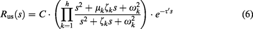
The modelling results of R_us(s) and R_ds(s) are shown in Tables 2 and 3 and Figures 5 and 6.

Table 2.

The parameters of R_us(s): h = 6.

k	ω k	ζ k	μ k
1	521.5	86.9	0.55
2	1508.0	558.5	0.55
3	2902.8	207.3	0.66
4	3707.1	285.2	0.78
5	4523.9	1005.3	0.47
6	5654.9	807.8	0.52
C = 0.95		$\tau \text{'}$  = 0.0045 s

Table 3.

The parameters of R_ds(s): h = 6, r = 6.

k	ω k	ζ k	μ k	l	ω l	ζ l	A l	B l	D l
1	565.5	94.2	0.35	1	439.8	110.0	0.0325	0	0
2	672.3	168.1	0.6	2	942.5	471.2	0.065	0	0
3	1822.1	1822.1	0.92	3	1759.3	879.6	0.05	0	0
4	1822.1	151.8	0.85	4	2576.1	1981.6	0.42	0.91	0.77
5	3141.6	209.4	0.46	5	2858.8	190.6	0.013	−0.016	0
6	3989.8	159.6	0.85	6	3248.4	81.2	7.75e-3	0	0
τ′= 0.014 s

Figure 5.

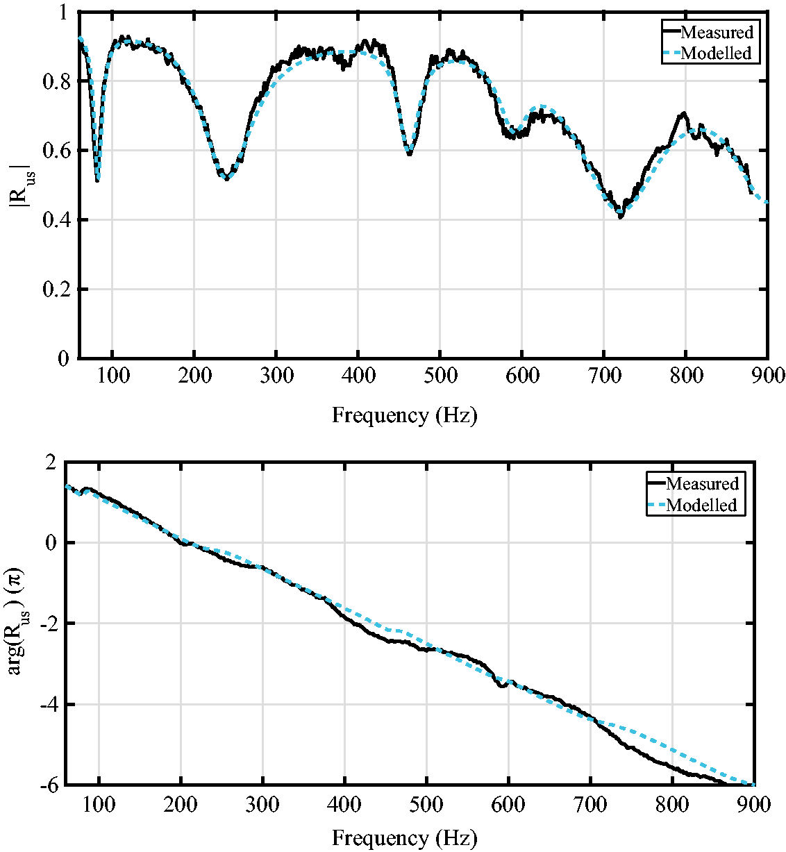
The modelling result of R_us(s): 12th order.

Figure 6.

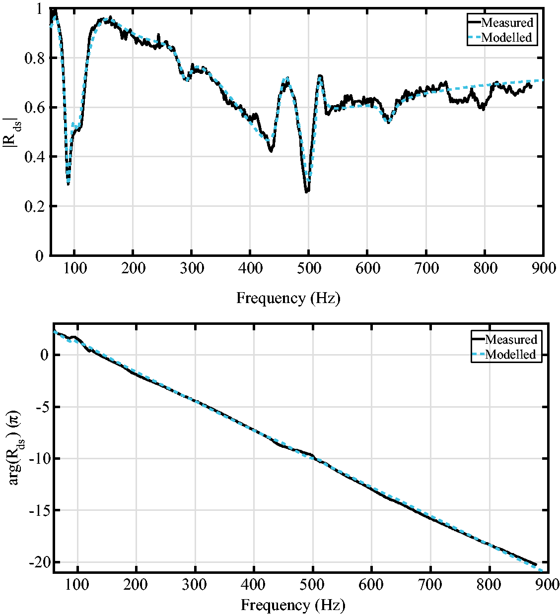
The modelling result of R_ds(s): 24th order.

Figures 5 and 6 show that the models match the measurements very well and are reliable for implementing the simulation of active control.

Control approach

Phase shift control

Phase shift control is a direct method to implement the active control of acoustic impedance. The basic principle is to measure the phase of the g-wave at $x_1$ . Next, the phase characteristics of downstream loudspeakers and the phase delay caused by sampling of DSP are compensated by the controller to guarantee that g_d generated by the downstream loudspeakers is nearly 180° out of phase with the measured signal. This principle can be described by equation (8)

$$\phi (i\omega )={\psi }_{\text{d}}(i\omega )-{\psi }_{\text{samp}}(i\omega )+\pi$$

(8)

where ϕ(iω) denotes the phase shift parameter for controller, which is calculated from ψ_d(iω) and ψ_samp(iω); ψ_d(iω) denotes the phase-frequency characteristic of the downstream loudspeakers, which can be obtained from the transfer function of G_d(s). The uncertainty of ψ_d(iω) depends on the modelling error of phase characteristic of G_d(s); ψ_samp(iω) denotes the phase delay caused by sampling of DSP. The value of ψ_samp(iω) is a function of the frequency of acoustic wave, which can be calculated by equation (9)

$${\psi }_{\text{samp}}(i\omega )=\frac{\omega }{f_{\text{samp}}}$$

(9)

where ω denotes the angular frequency of acoustic wave and f_samp denotes the sampling frequency of DSP, which is 18 kHz in this experiment. Equation (9) implies that when the sampling frequency of DSP is fixed, the higher ω is, the larger ψ_samp is. For example, when f = 60 Hz, ψ_samp is about 1.2°; when f = 600 Hz, ψ_samp is about 12°. In conclusion, when the frequency of acoustic wave is low, ψ_samp can be ignored; while when the frequency of acoustic wave is high, ψ_samp must be considered. The whole control frame for phase shift is shown in Figure 7 where r denotes the reference value. Because we aim to implement an anechoic end, r = 0. The phase shift controller consists of three parts: (1) phase shift Φ(s), (2) gain K₀, (3) bandpass filter Q(s). The bandpass filter’s function is to improve the gain margin (GM) of the whole control system, thereby avoiding instabilities. The transfer function of the phase shift process is given by equation (10)

$$\Phi (s)=\cos \phi (s)+\frac{\omega -s}{\omega +s}\sin \phi (s)$$

(10)

where ω denotes the angular frequency of acoustic wave. This phase shift module works only at a certain frequency ω, with a unit gain at ω.

Figure 7.

The phase shift control for acoustic impedance tuning.

ADRC

ADRC can be applied to control systems with complex uncertainties, including external nonlinear disturbance, modelling uncertainties, and unknown dynamics. The key idea of ADRC is to consider the external disturbance and the internal disturbance as a total disturbance. ²⁴ It can be estimated from the output characteristics of system and then compensated by ESO, implying that ADRC is model independent. ADRC includes linear ADRC and nonlinear ADRC. Nonlinear ADRC has better performance but parameter tuning is more complicated. By contrast, linear ADRC, especially the first-order ADRC and the second-order ADRC, has more applications in industrial control. The first-order ADRC will be discussed next.

Design of first-order ADRC

To establish the first-order ADRC for acoustic impedance tuning, suppose the system has the form of equation (11)

$$\dot{g}=\xi (t,g,\ddot{g},\mathrm{\dots },w)+bu$$

(11)

where g denotes the output of system, i.e. the g-wave in the duct; b denotes the gain factor of controller; w denotes disturbance; ξ denotes the dynamics of the system, including the state information, disturbances, and unknown dynamics of system. In most cases, the exact value of b is difficult to obtain. Thus, we use b₀ to estimate b. Equation (11) can be converted into the form of a state space

$$\dot{X}=AX+Bu+E\dot{\xi }$$

(12)

where $X\hspace{0.17em}=\hspace{0.17em}{[x_1,\hspace{0.17em}{x}_2]}^T\hspace{0.17em}=\hspace{0.17em}{[g,\hspace{0.17em}\xi ]}^T$ , $A\hspace{0.17em}=\hspace{0.17em}\left[\begin{array}{cc}0& 1\\ 0& 0\end{array}\right]$ , $B\hspace{0.17em}=\hspace{0.17em}{[b_0,0]}^T$ , and $E\hspace{0.17em}=\hspace{0.17em}{[0,1]}^T$ . To implement the tracking of g and ξ, ESO is designed as follows

$$\dot{Z}=AZ+Bu+L(g-z_1)$$

(13)

where $Z = {[z_1, z_2]}^T$ , z₁ tracks g, z₂ tracks ξ; and $L = {[{\beta }_1, {\beta }_2]}^T$ , which denotes the gain matrix of observer. For the convenience of parameter tuning and the asymptotic stability of control system, β₁ and β₂ are combined into a single parameter ω_o as follows

$$\{\begin{array}{l}{\beta }_1=2{\omega }_{\text{o}}\hfill \\ {\beta }_2={\omega }_{\text{o}}^2\hfill \end{array}$$

(14)

According to equation (13), ESO can be constructed as follows

$$\{\begin{array}{l}{\dot{z}}_1={\beta }_1(g-z_1)+z_2+b_{0}u\hfill \\ {\dot{z}}_2={\beta }_2(g-z_1)\hfill \end{array}$$

(15)

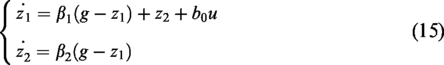
To obtain a model-independent control scheme, unknown dynamics ξ must be estimated by ESO. The control law can be designed as follows

$$u=\frac{-z_2+u_0}{b_0}$$

(16)

Thus, $\dot{g}\approx u_0$ , which is independent of the dynamics of system, u₀ can be controlled by a proportional process

$$u_0=k_{\text{p}}(r-z_1)$$

(17)

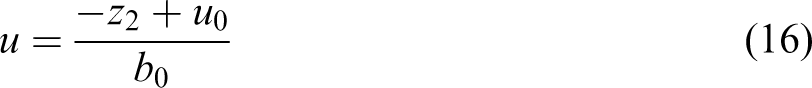
Thus, the first-order ADRC for acoustic impedance tuning can be designed as Figure 8.

Figure 8.

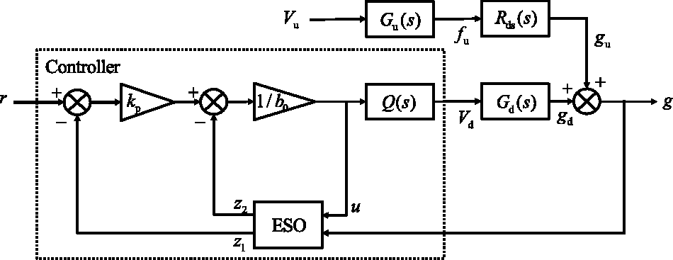
The first-order ADRC for acoustic impedance tuning. ESO: extended state observer.

Asymptotic stability analysis

Because ADRC is applied to control systems with uncertainties, we are interested in the stability of the control system. For the linear time invariant system, the stability can be determined by Routh–Hurwitz criterion. ³² As Figure 8 shows, ADRC for acoustic impedance tuning system includes G_d(s), which represents the transfer function of downstream loudspeakers. According to the modelling results in ‘Transfer function description of the test rig’ section, G_d(s) includes a time delay process with τ = 0.0060 s. So the acoustic impedance tuning system is nonlinear, and Routh–Hurwitz criterion is inapplicable. Here, the stability of ADRC is analysed with Lyapunov’s second method. ³³ Let $e\hspace{0.17em}=\hspace{0.17em}X\hspace{0.17em}-\hspace{0.17em}Z$ denote the tracking error of ESO, according to equations (12) and (13); the following is valid

$$\dot{e}=\tilde{\mathbf{A}}\mathbf{e}+E\dot{\xi }$$

(18)

where $\tilde{\mathbf{A}}$ satisfies

$$\tilde{\mathbf{A}}=A-LM$$

(19a)

$$M=\left[\begin{array}{cc}1& 0\end{array}\right]$$

(19b)

$\tilde{\mathbf{A}}$ has the form of

$$\tilde{\mathbf{A}}=\left[\begin{array}{cc}-{\beta }_1& 1\\ -{\beta }_2& 0\end{array}\right]$$

(20)

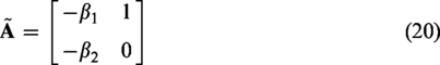
When equation (14) is satisfied, the real part of every eigenvalue of $\tilde{A}$ is negative, implying that $\tilde{A}$ is a Hurwitz matrix. Hence, the Lyapunov equation is applicable ³⁴

$${\tilde{\mathbf{A}}}^{\text{T}}P+\mathbf{P}\tilde{\mathbf{A}}\mathrm{=}-I$$

(21)

where P is a positive definite matrix. Thus, the Lyapunov function can be constructed as

$$V={(e-\eta )}^{T}P(e-\eta )$$

(22)

where V is a positive defined function; $\mathbf{\eta }\hspace{0.17em}=\hspace{0.17em}{[{\eta }_1, {\eta }_2]}^T$ satisfies

$$\dot{\mathbf{\eta }}-\tilde{\mathbf{A}}\mathbf{\eta }=\mathbf{E}\dot{\xi }$$

(23)

$\mathbf{\eta }$ has a solution in the sense of a Laplace transform

$$\{\begin{array}{l}{\eta }_1(s)=\frac{s}{s^2+{\beta }_{1}s+{\beta }_2}\xi (s)\hfill \\ {\eta }_2(s)=\frac{s(s+{\beta }_1)}{s^2+{\beta }_{1}s+{\beta }_2}\xi (s)\hfill \end{array}$$

(24)

Thus

$$\begin{array}{l}\frac{\text{d}V}{\text{d}t}={\left(\dot{e}-\dot{\eta }\right)}^{T}P\left(e-\eta \right)+{\left(e-\eta \right)}^{T}P\left(\dot{e}-\dot{\eta }\right)\\ ={\left(e-\eta \right)}^T\left({\tilde{A}}^{T}P+P\tilde{A}\right)\left(e-\eta \right)=-{\left(e-\eta \right)}^T\left(e-\eta \right)<0\end{array}$$

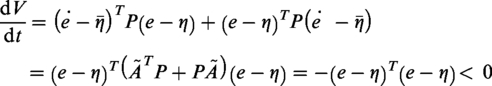
The equation implies that dV/dt is a negative defined function. Thus, the control system is asymptotic stable in any cases, even if the characteristic of system is unknown. When 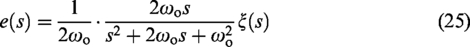$t\to \infty$ , $\mathbf{e}\to \mathbf{\eta }$ , which implies the static tracking error has a form of

$$e(s)=\frac{1}{2{\omega }_{\text{o}}}\cdot \frac{2{\omega }_{\text{o}}s}{s^2+2{\omega }_{\text{o}}s+{\omega }_{\text{o}}^2}\xi (s)$$

(25)

where $\frac{2{\omega }_{o}s}{s^2+2{\omega }_{o}s+{\omega }_o^2}$ has a unit gain at ω_o. Equation (25) implies that, as ω_o increases, the static tracking error of ESO is reduced. In addition to the stability, the convergence rate, which is related to the quality of control, is also crucial. Regarding the first-order ADRC, $\tilde{\mathbf{A}}$ has a double eigenvalue, −ω_o, which can be used to estimate the convergence rate.

Parameter tuning method

The first-order active disturbance rejection controller has three parameters to tune: ω_o, k_p, and b₀. To achieve good performance, parameter tuning should obey the following principles:

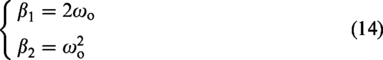
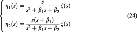
As mentioned in ‘Asymptotic stability analysis’ section, β₁ and β₂ are tuned by ω_o, which is the gain of ESO. Larger ω_o results in smaller static tracking error and higher rapid convergence rate, whereas excessively large ω_o causes instability. Thus, ω_o should be gradually increased to a reasonable value in the condition of secured stability. For a real control system, the value of ω_o should not exceed the sampling frequency of controller; otherwise will lead to instability.

k_p is the ratio of the output state estimation z₁ and z₂. A larger k_p implies a stronger control signal, whereas an excessively large k_p causes system instability. Moreover, k_p can weakly change the phase characteristic of the controller, which depends on other parameters.

b₀ is related to the gain of control output. The control effect increases as 1/b₀ rises and the system responds more rapidly, implying a better performance. However, excessively small b₀ also results in system instability because the GM is reduced. This problem can be solved by adding a bandpass filter, as discussed in detail in the following section.

GM and bandpass filter

In the preceding discussion, phase shift control and ADRC are introduced, and a bandpass filter is added to the control system to extend the range of parameter tuning of the controller. In this part, we will figure out the reason.

In general, the parameter tuning range of a controller depends on the GM of a system. The larger the GM of the system, the larger the tuning range is, implying better performance of control. The GM is defined as equation (26a)

$$\text{GM }(\mathrm{dB})=-20{\log }_{10}|G(j{\omega }_{\text{c}})|$$

(26a)

where ${\omega }_c$ is called the crossover frequency (CF), which satisfies

$$\angle G(j{\omega }_{\text{c}})=-180°$$

(26b)

The GM of system can be determined by the Nyquist plot of the open loop transfer function of the system, as shown in Figure 9.

Figure 9.

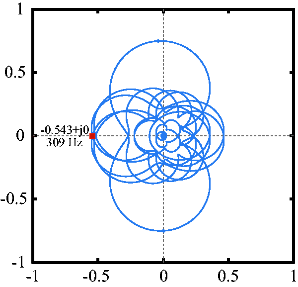
The Nyquist plot of G_d(s): the crossover point is −0.543 + j0; the CF f_c = 309 Hz.

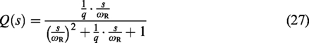
According to the crossover point shown in Figure 8, we find that GM = 5.3 dB, which implies that the gain of controller should not exceed 5.3 dB; otherwise the control system will become unstable. To avoid instability, a bandpass filter is added to the control loop. A typical second order bandpass filter can be described by equation (27)

$$Q(s)=\frac{\frac{1}{q}\cdot \frac{s}{{\omega }_{\text{R}}}}{{\left(\frac{s}{{\omega }_{\text{R}}}\right)}^2+\frac{1}{q}\cdot \frac{s}{{\omega }_{\text{R}}}+1}$$

(27)

where ω_R denotes the resonance frequency and q denotes the quality factor, which is defined as the ratio of the resonance frequency to the bandwidth. The Bode plot and the Nyquist plot of the bandpass filter are shown in Figure 10.

Figure 10.

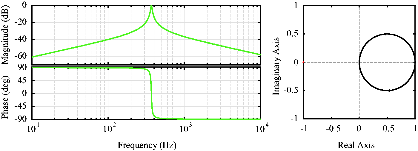
The Bode plot and the Nyquist plot of the bandpass filter.

Figure 10 reveals that a bandpass filter has an infinite GM. When the bandpass filter is added to the loop, the GM of total system is increased. The larger q is, the larger GM is. To generalize the conclusion in a precise manner, an estimation of the relationship between GM and q is to be developed when q is sufficiently large.

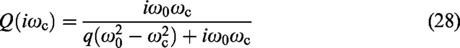
Suppose that the CF of system is ω_c; thus, the response of the bandpass filter at ω_c is given by equation (28)

$$Q(i{\omega }_{\text{c}})=\frac{i{\omega }_0{\omega }_{\text{c}}}{q({\omega }_0^2-{\omega }_{\text{c}}^2)+i{\omega }_0{\omega }_{\text{c}}}$$

(28)

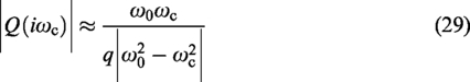
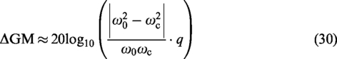
When q is sufficiently large, $|q({\omega }_0^2\hspace{0.17em}-\hspace{0.17em}{\omega }_c^2)|\hspace{0.17em}\gg \hspace{0.17em}\left|i{\omega }_0{\omega }_c\right|$ ; thus

$$\left|Q(i{\omega }_{\text{c}})\right|\hspace{0.17em}\approx \hspace{0.17em}\frac{{\omega }_0{\omega }_{\text{c}}}{q\left|{\omega }_0^2-{\omega }_{\text{c}}^2\right|}$$

(29)

When f₀ = 370 Hz, f_c = 420 Hz, q = 30, there is |Q(iω_c)| ≈l 0.13, and the gain at f₀ remains 1. This result implies an increment of GM, which can be estimated by equation (30)

$$\Delta \text{GM}\hspace{0.17em}\approx \hspace{0.17em}20{\log }_{10}\left(\frac{\left|{\omega }_0^2-{\omega }_{\text{c}}^2\right|}{{\omega }_0{\omega }_{\text{c}}}\cdot q\right)$$

(30)

where $\Delta \mathrm{GM}$ denotes the increment of GM. Equation (30) is applicable to any self-stable system when q is very large compared to $\frac{{\omega }_0}{2|{\omega }_c - {\omega }_0|}$ . This asymptotic relationship between GM and q can be verified by Figure 11.

Figure 11.

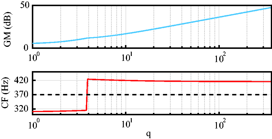
The relationships among q, GM (top) and CF (bottom). CF: crossover frequency; GM: gain margin.

Figure 11 shows that as q increases, GM tends to increase, implying that the performance of control is improved. The CF tends to a constant, mainly because the phase-frequency characteristic of bandpass filter tends to a constant (±90°) when q is very large.

Briefly, to extend the range of parameter tuning of controller, a bandpass filter is desired. A filter with larger q value is better. However, if q is too large, it becomes very difficult to realize. In this paper, a filter with q = 30 is applied to the control system.

Results and analysis

The active control simulations and experiments are conducted in a frequency range from 60 to 650 Hz. The total results are shown in Figure 12.

Figure 12.

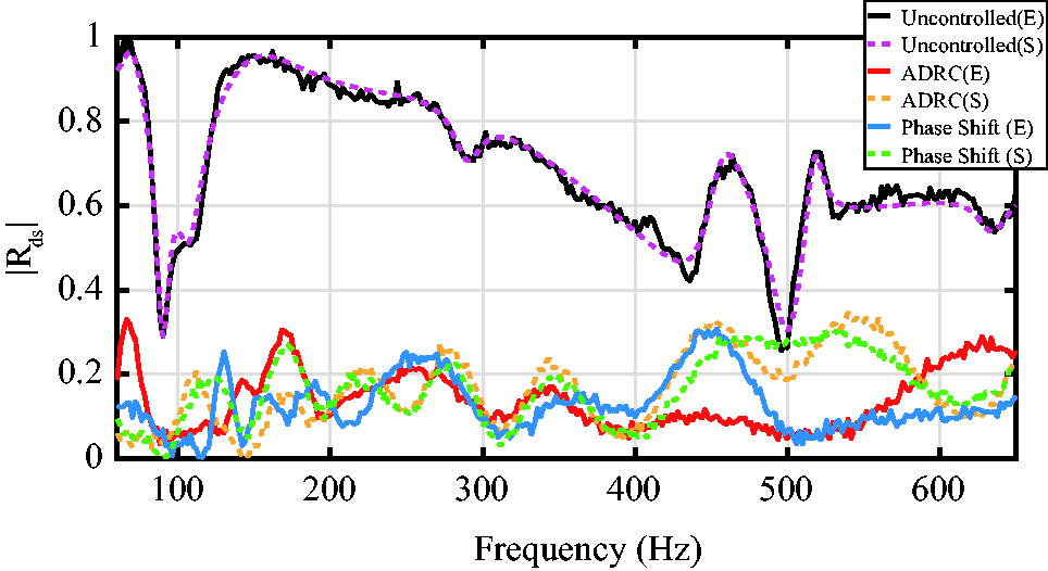
The experimental and simulation results of ADRC and phase shift control: E denotes experiment and S denotes simulation. ADRC: active disturbance rejection control.

Figure 12 shows that the simulation results are in good agreement with the experimental results over a wide frequency range, especially from 100 to 400 Hz. The results show that ADRC and phase shift control have a similar performance on acoustic impedance tuning: the downstream reflection coefficient can be reduced to 0.1–0.2 on average. But this result does not imply that phase shift control and ADRC are equally good. There is another important question we did not consider: a precise model of G_d(s) is necessary for phase shift control, whereas ADRC is model independent, which implies that the properties of the system are not considered. To determine the dependence of phase shift control on the model, a fuzzy model of G_d(s) is established and compared to the precise model, as shown in Figure 13.

Figure 13.

The precise model (27th order) and fuzzy model (17th order) of G_d(s).

The experiment result is shown in Figure 14.

Figure 14.

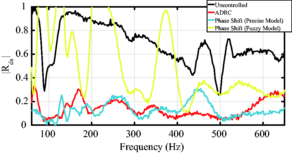
The influence of the accuracy of the model on the performance of the phase shift control. ADRC: active disturbance rejection control.

As shown in Figure 14, when a fuzzy model is applied to the phase shift control, the control performance deteriorates significantly. In some cases, the reflection coefficient is even increased. The reason is in phase control, the value of phase compensation is given by the model of G_d(s) while the reduction produced by phase matching is sensitive to the phase error. ³⁵ Compared to the precise model, the fuzzy model of G_d(s) has larger modelling error, especially from 60 to 400 Hz (Figure 13). As a result, we can find a significant deterioration of performance from 60 to 400 Hz (Figure 14). At the same time, the performance from 400 to 650 Hz is not so bad, since the phase error of fuzzy model during 400–650 Hz is relatively small. In conclusion, ADRC is model independent, whereas phase shift control needs accurate model. So ADRC is superior when there is no accurate model or when there is serious system uncertainty.

Moreover, Figure 12 shows that |R_ds| can be suppressed to 0.1–0.2 by ADRC, which is nearly the lowest level under existing conditions. Here, we will figure out the limitations on reducing |R_ds|. In the frame of first-order ADRC, there are two approaches to further reduce |R_ds|:

Increase ω_o. As mentioned in ‘Asymptotic stability analysis’ and ‘Parameter tuning method’ sections, ω_o reflects the tracking quality of ESO. If ω_o is increased, the tracking error of ESO would be reduced, thus |R_ds| can be suppressed lower. However, ω_o is limited by the sampling frequency of DSP, i.e. f_samp. If ω_o exceeds f_samp, system would become unstable.

Increase k_p or 1/b₀. These two parameters represent control gain. If control gain is increased, the control signal would become stronger, thus |R_ds| can be suppressed lower. However, control gain cannot be increased infinitely: it should not exceed the GM of system, otherwise instability would happen, which is shown as the phenomenon of beating oscillation (Figure 15).

Figure 15 shows the transition of stable state in ADRC, which is achieved by tuning b₀ from 280 to 230. In critical unstable state, there is a low-frequency oscillation on the amplitude of g. The frequency spectrum is shown in Figure 16, from which we can find that a peak at 414 Hz is excited. This is because the Nyquist curve of system cross over −1 + j0 point at 414 Hz (CF), when q = 30 (Figure 10). As a result, signal at 414 Hz is amplified greatly, and control system breaks down. In addition, the frequency of beating oscillation equals to the difference between main frequency and CF.

Figure 15.

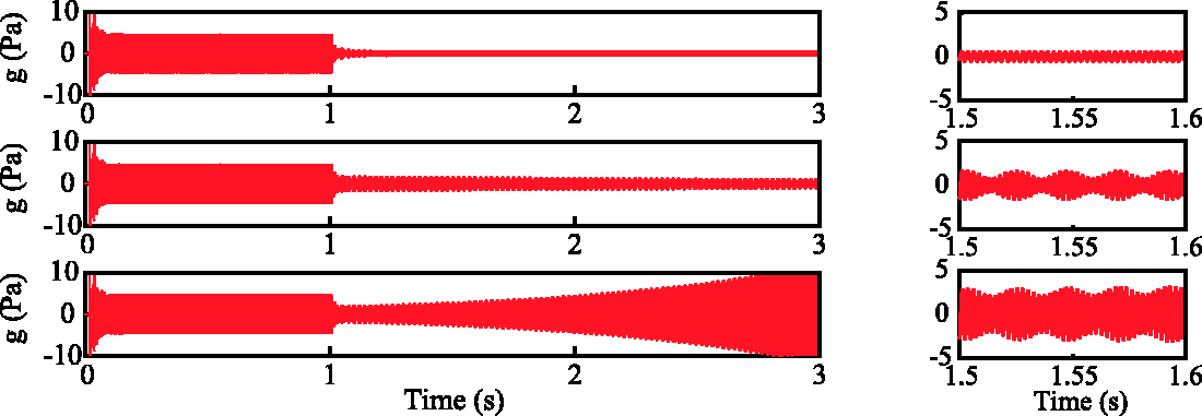
Phenomenon of instability in ADRC caused by increasing 1/b₀ overly: f = 370 Hz, q = 30; stable (top, b₀ = 280), critical instable (middle, b₀ = 234); and instable (bottom, b₀ = 230).

Figure 16.

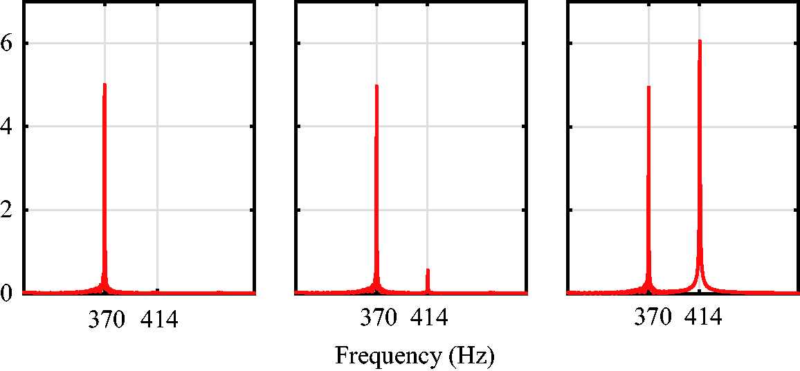
The frequency spectrum of g-wave: stable (left), critical instable (middle), and instable (right).

In conclusion, for further reducing | R_ds |, the sampling frequency of DSP and the GM of system are main limitations. According to the analysis in ‘GM and bandpass filter’ section, the GM of system can be improved by increasing the q value of bandpass filter. However, if q is too large, it is difficult to realize in practice. Besides, ESO in high-order ADRC can track the system more precisely. Thus, high-order ADRC for acoustic impedance tuning is promised to achieve better performance, which remains to be investigated in further researches.

Conclusion and outlook

In this paper, to achieve an anechoic end on an acoustic test rig, a solution of the first-order ADRC for acoustic impedance tuning was proposed and compared with the phase shift control. The results of the simulation and the experiment showed that the reflection coefficient can be suppressed to 0.1–0.2 by applying ADRC. Different from the previous approaches, ADRC for impedance tuning was proposed as a model-independent solution for the first time. To investigate the model dependence, a precise model and a fuzzy model were established. The experimental results showed that the performance of phase shift control is strongly influenced by the accuracy of the model, and the precise model of system is unnecessary for ADRC. Briefly, when the actual system is too complicated to describe, ADRC is a much more effective strategy than phase shift control. For the reliability of the simulation, the test rig is described by a 27th order transfer function. For further research, high-order ADRC for acoustic impedance tuning is desired to investigate whether a better performance can be achieved on high-order systems.