Sage Journals: Discover world-class research

Abstract

Rolling bearing is one of the most crucial components in rotating machinery and due to their critical role, it is of great importance to monitor their operation conditions. However, due to the background noise in acquired signals, it is not always possible to identify probable faults. Therefore, signal denoising preprocessing has become an essential part of condition monitoring and fault diagnosis. In the present study, a hybrid fault diagnosis method based on singular value difference spectrum denoising and local mean decomposition for rolling bearing is proposed. First, as a denoising preprocessing method, singular value difference spectrum denoising is applied to reduce the noise of the bearing vibration signal and improve the signal-to-noise ratio. Then, local mean decomposition method is used to decompose the denoised signals into several product functions. And product functions corresponding to the fault feature are selected according to the correlation coefficient criterion. Finally, Teager energy spectrum is analyzed by applying the Teager energy operator to the constructed amplitude modulation component. The proposed method is successfully applied to analyze the vibration signals collected from an experimental motive rolling bearing and rolling bearing of the self-made rotor experimental platform. The experimental results demonstrate that the proposed singular value difference spectrum denoising and local mean decomposition method can achieve fairly or slightly better performance than the normal local mean decomposition-Teager energy operator method, fast kurtogram, and the wavelet denoising and local mean decomposition method.

Keywords

Rolling bearing fault feature extraction singular value difference spectrum local mean decomposition Teager energy operator

Introduction

Rolling bearing is one of the most important components and most easily damaged parts in rotating machinery. When there is a fault on rolling bearing, it will affect the normal operation of mechanical equipment and even lead to a serious accident. Therefore, the fault diagnosis of rolling bearing is particularly important.¹ When a localized defect occurs on rolling bearing surfaces, a series of impulses are created in vibration signal of a rolling bearing. These impulses excite the resonances of the system with a certain repetition frequency. However, the operation process of rolling bearing is a complex and unsteady dynamic process; the feature of vibration signal in time domain and frequency domain will be submerged by noise.² Therefore, a desirable and successful diagnostic method which can clearly extract the fault feature from the vibration signal of rolling bearing should be able to detect the corresponding repetition frequency of the impulse sequence.

In the process of feature extraction, demodulation of the original signal with envelope analysis can reveal additional fault-related features.³ As a noticeable faulty feature, repetitive transients have been extensively investigated for fault diagnosis of rotating machinery. Owing to the abilities to indicate not only non-Gaussian components in a signal but also their locations in frequency domain, spectral kurtosis (SK) is effective for extracting repetitive transients and has attracted considerable attention.⁴ Antoni^5,6 conducted intensive research based on SK and proposed a time–frequency analysis method named “kurtogram” which can be described as a cascade of SK calculated by short-time Fourier transform with different time window lengths. To make online industrial applications accessible, fast kurtogram (FK) was developed, which presented adequate efficiency in transient fault detection.⁷ The impulses are extracted and highlighted after the raw signal is processed by the band filter of which the center frequency and bandwidth are optimized by FK. Barszcz and Randall⁸ adopted FK to detect the tooth crack in the planetary gear of a wind turbine and . Zhang and Randall⁹ combined genetic algorithms and FK to optimize the parameters of the band filter in fault diagnosis for rolling bearing. Wang et al.¹⁰ combined the minimum entropy deconvolution and FK for rolling bearing early stage fault feature extraction in early stage. Despite the efficiency, FK reveals its weakness when there are strong nonstationary interference contents in the raw signal.¹¹ In addition, when the decomposition level is confirmed, the center frequency and the frequency resolution taken into consideration are limited. Namely, the optimal filter is nominal. Afterward, many fast detection algorithms have been applied to process repetitive transients caused by bearing rolling element defects and gear defects, such as the improved kurtogram,¹² the enhanced kurtogram,¹³ the sparsogram,¹⁴ and the infogram.¹⁵ However, kurtogram is very sensitive to large random impulses and the selected frequency band with maximum kurtosis may be dominated by such random impulses.¹⁶

In order to solve this problem the demodulation methods based on, Hilbert transform and Teager energy operator (TEO) demodulates are also most widely used .¹⁷ Envelope demodulation based on a single amplitude modulation (AM) frequency modulation signal has been widely used in the field of voice recognition^1,18 and fault diagnosis.^1,19,20 However, the vibration signal of rolling bearing is a multicomponent AM–FM signal. Therefore, the vibration signal of rolling bearing should be decomposed into multiple single AM–FM signals in the process of envelope demodulation. The most frequently used signal decomposition methods are wavelet decomposition, empirical mode decomposition (EMD), ensemble empirical mode decomposition (EEMD), and so on. Among them, EMD and EEMD are self-adaptive decomposition methods based on the character of signal, and they have been widely researched and used in the field of fault diagnosis and pattern recognition. Zhang et al.²¹ have utilized EMD to eliminate the noise of stator current signal which was generated by a broken rotor bar. Then, Hilbert transform is used to extract the envelope of denoised signal. Finally, the fault characteristic frequency of broken rotor bar is extracted based on envelope FFT spectrum. To overcome the weakness that traditional envelope analysis should determine resonant frequency, Tsao^22,23 has proposed a method combined EMD with Hilbert transform. In view of the fact that the gear signal of fan-driven generator is a multicomponent signal and is seriously polluted by noise, a fault diagnosis method combined EEMD with TEO has been proposed.²⁴

On the basis of EMD and EEMD, Smith²⁵ has proposed a new self-adaptively unsteady signal decomposition method, named local mean decomposition (LMD). This method can handle the negative frequency, problem that it cannot explain in EMD method. At the same time, it is less sensitive to boundary effect and mode mixing compared with EMD and EEMD.²⁶ This is a reason why it is widely used in the flied of fault diagnosis. Cheng has introduced LMD method to decompose multicomponent AM–FM signal of the main components of rotating machinery (rotor, gear, and rolling bearing) into several product functions (PFs). And then the operation states of bearing have been identified by computing the instantaneous frequency of PFs and compared the identification performance with the EMD method.^27,28 Liu et al.²⁹ have used LMD method to decompose the vibration signal of generator fault into several PFs and realized the early period fault diagnosis of generator in low-speed vibration of motor. In order to select useful PFs to describe the operation state of machine, a new fault diagnosis method combining LMD with FFT is proposed.³⁰ In conclusion, the LMD method has been widely used in many fields, especially in the field of condition monitoring and fault diagnosis of rotating machinery.²⁸ ^,31 However, the noise is generally unavoidable, which is usually introduced into signals by various interference factors, such as the external environment and testing instrument, etc.³² Since impulses containing fault information can be concealed by unavoidable noise, noise will affect processing results and the application effects of fault diagnosis methods for rolling bearing. In particular, in industrial environments, vibration signals can be covered with heavy background noise originated from measurement system as well as due to misalignment, unbalance, crack(s) on the rotating shaft, looseness, and distortions.²² Then, the LMD method is greatly influenced by noise, mostly to increase a lot of extra, useless frequency component, etc.³³ Therefore, denoising signal processing is required before envelope analysis. The ideal denoising technique should remove the noise from the acquired signal without distorting the essential characteristics of the signal. Various techniques such as moving average, short-duration averaging, etc. are used to improve the signal signal-to-noise ratio (SNR) to some extent.^32,34–39 Among all the denoising methods, wavelet transform (WT) denoising and singular value difference spectrum (SVDS) denoising has been widely applied to many signals.³⁵ Different from WT denoising, SVDS denoising is a nonparametric signal analysis tool which can be implemented without predefined base functions. Through correlation analysis, SVDS is able to reveal the weak intrinsic pattern buried in a signal and effectively suppress the noise with different distributions.^40,41 At the same time, the noise elimination algorithm based on SVDS is relatively fast and easy to implement. SVDS-based feature extraction method or singular spectrum analysis (SSA) enables a suitable opportunity to monitor the singular values obtained from vibration signals at different operation conditions.⁴²

Based on the above analyses, a hybrid fault diagnosis method is proposed for rolling bearing based on SSA and LMD. The structure of this paper is organized as follows. The next section introduces background theory of the proposed method. “The fault feature extraction process of SVDS–LMD–TEO” section describes the proposed hybrid fault diagnosis method. “Experimental results” section gives experimental validation and engineering application. Finally, conclusions and future works are drawn in the final section.

Background theory

The denoising method based on SVDS method

SVDS is a numerical method which states that a matrix A of rank L can be decomposed into the product of three matrices, an orthogonal matrix U, a diagonal matrix S, and the transposed matrix V^T of an orthogonal matrix V.⁴³ This method is usually presented as follows

A_{m \times n} = U_{m \times m} * S_{m \times n} * V_{n \times n}^{T}

(1)

where U^TU = I and V^TV = I, S is a diagonal matrix containing the square roots of eigenvalues of A^TA, which can be expressed as S = diag(σ₁, σ₂, …, σ_L), and L = min(m, n). σ_i (i = 1, 2, …, L) is called the singular values of the matrix A.

The method presented in Tufts et al.⁴⁴ offers a possibility to find the best approximation of the original data points using fewer dimensions by SVDS. Therefore, it can be used as a process for data reduction and this makes the SVDS a useful tool for denoising of vibration signals. There exists an m× n matrix A of rank $l \leq L$ , which minimizes the sum of the squared error between the elements of the matrix A and the corresponding elements of the matrix A which can be formed as

A_{new} = U_{l} * S_{l} * V_{l}^{T}

(2)

where A_new is the reconstructed matrix using only the largest l number of singular values and the rest of the singular values are replaced by zero. It shows that the essence and key of SVD is the correct choice of the largest l number of singular values. Therefore, the SVDS is introduced to eliminate the noise of vibration signal. The implementation process of the SVDS is as follows.

Step 1: The original vibration signal is constructed to Hankel matrix and decomposed by SVD.

Step 2: The singular values which consist of the diagonal element of matrix S are sorted. According to the order from large to small, a new sequence S_new=[σ₁, σ₂,…, σ_q] is obtained.

Step 3: The SVDS b_i is calculated according to equation (3)

b_{i} = σ_{i} - σ_{i + 1}, i = 1, 2, \dots, q - 1

(3)

where q is the number of singular value in difference spectrum (q = L−1).

Step 4: The mutation or sharp change point l is selected in the SVDS. In other words, the first l number of singular values represent the desired extraction signal.

LMD method

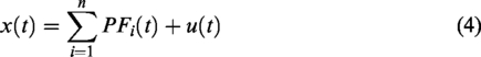
The LMD adaptively decomposes a multicomponent signal into a number of PFs. A PF, with a physical meaning, is the product of an amplitude envelope signal and a frequency-modulated signal. The complete time–frequency distribution of the analyzed signal could be obtained by assembling the instantaneous amplitude and instantaneous frequency of all PFs. As a result, the analyzed signal x(t) can be represented as

x (t) = \sum_{i = 1}^{n} P F_{i} (t) + u (t)

(4)

where i is the number of the PFs and u(t) represents the residual term. The more detail about LMD can be found in Smith.²⁵

Envelope demodulation of signal

Analyze the principle of envelope demodulation of signal

The method of envelope demodulation analysis implied envelope detection and spectrum analysis of signal comprehensively. The envelope demodulation methods commonly are used to recognize fault of machinery according to the spectral peak of the envelope spectrum. In fact, the high frequency intrinsic vibration is regarded as the carrier of vibration signal of rolling bearing. The amplitude will be demodulated by the pulse excitation force caused by the drawbacks, and the final vibration signal of bearing is a complex AM–FM waveform. The modulation frequency of modulation wave is the corresponding through frequency of drawback. Thus, the frequency component of modulation waveform contains the fault frequency of corresponding drawback. It makes it possible to realize the fault diagnosis of bearing by using envelope demodulation.

Correlation analysis

The LMD method has been widely used to process nonlinear signal for its adaptive filtering properties and multiresolution, but there will be false or redundant components in the decomposition process. The correlation coefficient between PFs and the original signal x(t) is introduced to solve this problem and decide which PFs should be retained and which PFs should be removed.

The correlation coefficient cor(t) between PFs and the original signal x(t) is calculated by the following equation³⁸

c o r (t) = \frac{\sum_{t = 1}^{2 N - 1} P F_{j} (t) x (t)}{\sqrt{\sum_{t = 1}^{2 N - 1} P {F_{j}}^{2} (t) \sum_{t = 1}^{2 N - 1} x^{2} (t)}}

(5)

where N is the length of the signal and j is the jth PF.

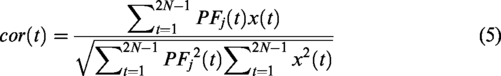
Generally speaking, the criterion to determine the linear correlation of two variables can be concluded as: 0 ≤ cor(t) <0.3 is weakly correlated. 0.3 ≤ cor(t) < 0.5 is lowly correlated. 0.5 ≤ cor(t) < 0.8 is significantly correlated. 0.8 ≤ cor(t) ≤1 is highly correlated. Therefore, the larger the value of cor(t), the higher the degree of correlation. To not lose any useful information, in this paper, we defined that the threshold value of the correlation coefficient cor(t) is larger than 0.3. In other words, the PFs, with cor(t)≥0.3, can be selected as efficient components.

TEO demodulation

For the continuous signal x(t), TEO demodulation principle is as follows⁴⁵

φ [x (t)] = {[\dot{x} (t)]}^{2} - x (t) \ddot{x} (t)

(6)

where

\dot{x} (t)

and

\ddot{x} (t)

are the first-order differential and the second-order differential corresponding.

For discrete signal x(n), the differential operation is replaced with difference operation. Then TEO operator $ϕ [x (n)]$ can be defined as

ϕ [x (n)] = {[x (n)]}^{2} - x (n - 1) x (n + 1)

(7)

From equation (7), for any given discrete signal x(n), the TEO calculates the energy of signal resource at any time n only by using the data of three samples. The TEO energy $ϕ [P F]$ of PF components can be calculated according to equation (7). Then, the fault feature will be extracted from the Fourier spectrum of the $ϕ [P F]$ .

The fault feature extraction process of SVDS–LMD–TEO

The proposed singular value difference spectrum denoising and local mean decomposition (SVDS–LMD) method combines the SVDS denoising with LMD method, which adaptively decomposes signals into various time scales. The flowchart of the proposed method is illustrated in Figure 1. The procedure is as follows.

Figure 1.

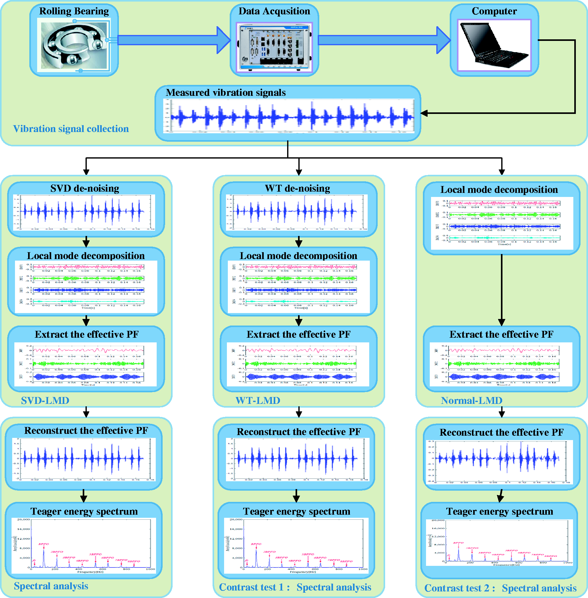
Flowchart of the implementation process of the proposed method. PF: product function; SVDS–LMD: singular value difference spectrum denoising and local mean decomposition; WT–LMD: wavelet denoising and local mean decomposition.

Step 1: Remove the noise of the collected vibration signal of rolling bearing by using SVDS to obtain a high SNR signal sequence x_d(t).

Step 2: The signal sequence x_d(t) is decomposed into k number of PFs using the LMD method.

Step 3: The interested or efficient PFs are selected based on correlation coefficient criterion.

Step 4: Reconstruct the efficient PFs to obtain the subsequent analysis signal x_new(t).

Step 5: The reconstructed signal x_new(t) is processed by TEO and then the characteristic frequencies of rolling bearing are identified according to the Teager energy spectrum.

Experimental results

In order to verify the effectiveness of the proposed SVDS–LMD method, the experimental simulation signal and the actual test signal collected from the rolling bearing with crack damage are applied to the experimental verification. Furthermore, a comparison of the normal LMD method, WT–LMD, FK and the proposed SVDS–LMD method is described in this section.

Experimental verification

Data acquisition

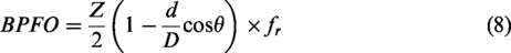
The experimental platform consists of a 2 hp motor, a torque sensor/decoder, a power tester, and an electronic controller (not shown in Figure 2).⁴⁶ The acceleration sensor is installed on the motor drive port, the motor speed is 1797 r/min (namely, the rotational frequency f_r is 1797/60 Hz =29.95 Hz). The sampling frequency f_s of the data acquisition system is 12 kHz and the experimental data length N is 2048. The test bearing parameters are shown in Table 1. Then, the defect frequency of rolling bearing is calculated according to equations (8) to (10),⁴⁷ respectively. The calculation results are summarized as follows: Ball Pass Frequency Outer(BPFO) = 107.36 Hz, Ball Pass Frequency Outer (BPFI) = 162.19 Hz, and Ball Spin Frequency (BSF) = 141.17 Hz.

B P F O = \frac{Z}{2} (1 - \frac{d}{D} \cos θ) \times f_{r}

(8)

Inner ring defect frequency: B P F I = \frac{Z}{2} (1 + \frac{d}{D} \cos θ) \times f_{r}

(9)

Rolling defect frequency: B S F = \frac{D}{2 d} (1 - {(\frac{d}{D} \cos θ)}^{2}) \times f_{r}

(10)

Figure 2.

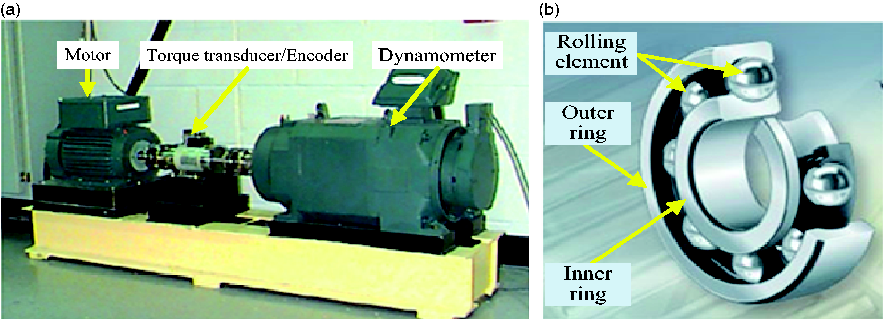
Bearing test rig and rolling bearing. (a) Bearing test rig and (b) rolling bearing.

Table 1.

The 6205-2RSJEMSKF bearing parameters.

Rolling element number (Z)	Inner ring diameter (in.)	Outer ring diameter (in.)	Contact angle (θ)	Rolling element diameter d (in.)	Pitch diameter D (in.)
9	0.9843	2.0472	0°	0.3126	1.537

Results and analysis

The vibration signal of rolling bearing, such as normal running condition, outer ring fault, inner ring fault, and rolling element fault, is selected, respectively. In order to simulate the early failure of the outer ring, inner ring, and rolling element, the vibration signal with smaller diameter of 0.007 in. (about 0.01778 cm) is selected.

Normal operation

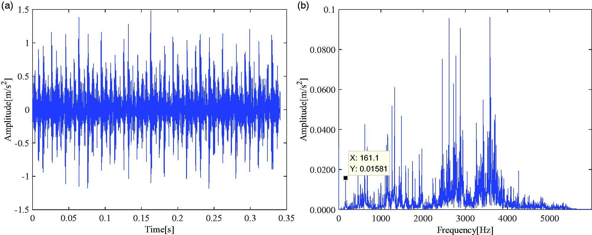
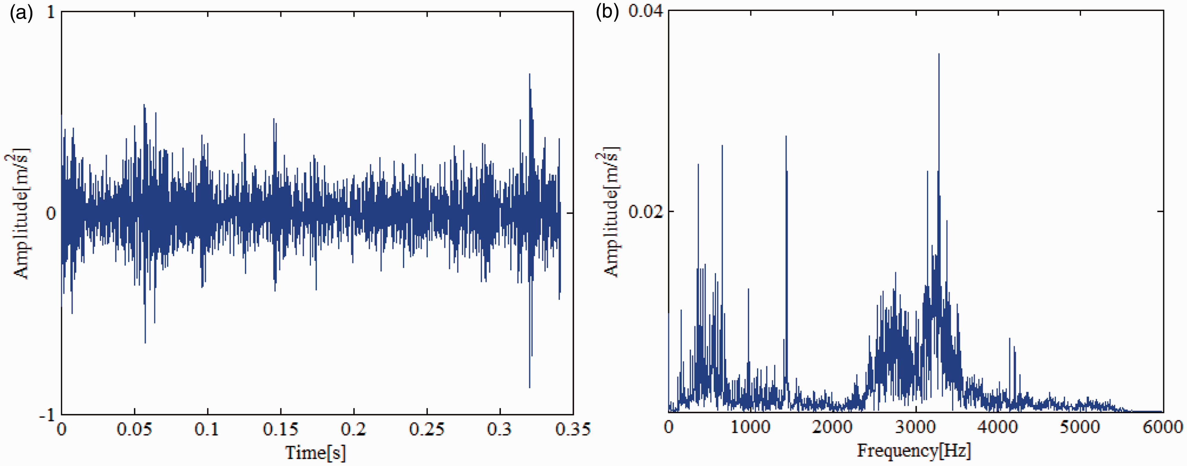
Figure 3 shows the time-domain waveform and the FFT spectrum of the raw vibration signal collected from the tested bearing in Figure 2. It can be seen that the condition features are buried in the background noise and the working conditions of the rolling bearing are difficult to be identified. Therefore, the normal LMD method, WT–LMD method, FK and the proposed SVDS–LMD method are applied to analyze this vibration signal, respectively.

Figure 3.

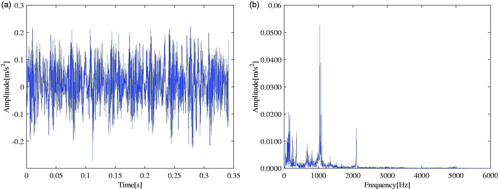
The time waveform and its corresponding FFT spectrum of the normal operation. (a) Time-domain waveform and (b) FFT spectrum. FFT: fast Fourier transform.

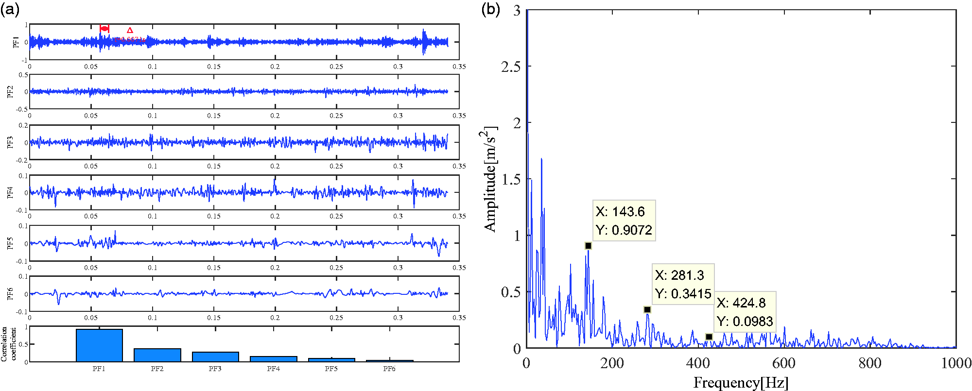
Figure 4 shows the results of the normal LMD method. Because the first six PFs contain almost all fault information, other PFs and residual are omitted. Moreover, the correlation coefficients between the first six PFs and original vibration signal x(t) are calculated through equation (5) and shown in Table 2. The correlation coefficients of “PF1–PF2” are greater than 0.3, and PF1 and PF2 are selected as the effective components. As shown in Figure 4(a), it also can be seen that the periodical impulse of PF1 and PF2 is approximately equal to 0.034 seconds, which mainly corresponds to the rotational frequency (f_r=29.95 Hz) of the tested rolling bearing. Therefore, PF1 and PF2 are selected to reconstruct the subsequent signal x_new(t). Figure 4(b) shows the Teager energy spectrum of x_new(t) and the axis x only shows the valid range 0–600 Hz. The rotational frequency f_r of rolling bearing and its harmonics 2f_r can be identified. The results show that the rolling bearing is well operated without failure.

Figure 4.

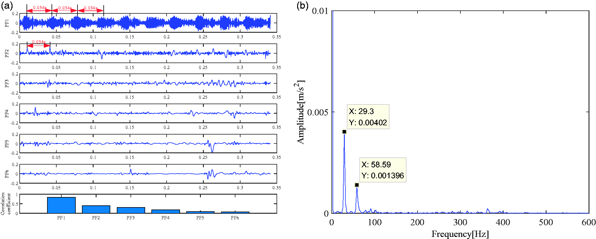
The analysis results of normal LMD method. (a) Decomposition results and (b) Teager energy spectrum.

Table 2.

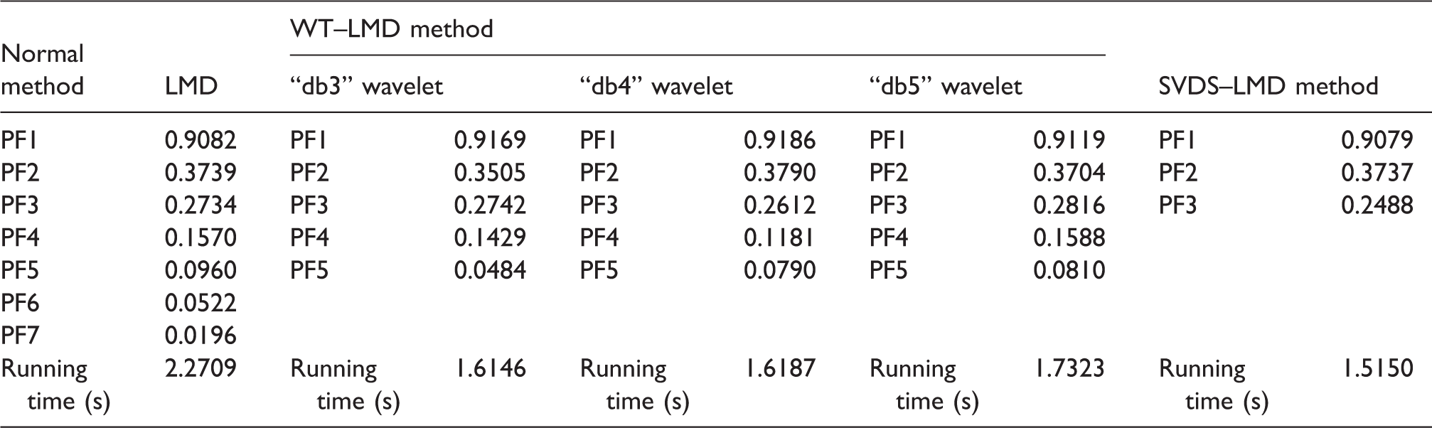
The correlation coefficients of PFs and the decomposed original signal x(t).

Normal method	LMD	WT–LMD method
Normal method	LMD	“db3” wavelet		“db4” wavelet		“db5” wavelet		SVDS–LMD method
PF1	0.8413	PF1	0.9598	PF1	0.8494	PF1	0.8444	PF1	0.8418
PF2	0.4023	PF2	0.2606	PF2	0.3811	PF2	0.4199	PF2	0.4115
PF3	0.2967	PF3	0.1163	PF3	0.2358	PF3	0.3156	PF3	0.2759
PF4	0.1849			PF4	0.1071	PF4	0.1203	PF4	0.1788
PF5	0.0922					PF5	0.1540
PF6	0.0675
Running time (s)	1.9134	Running time (s)	1.4841	Running time (s)	1.6216	Running time (s)	1.8091	Running time (s)	1.6302

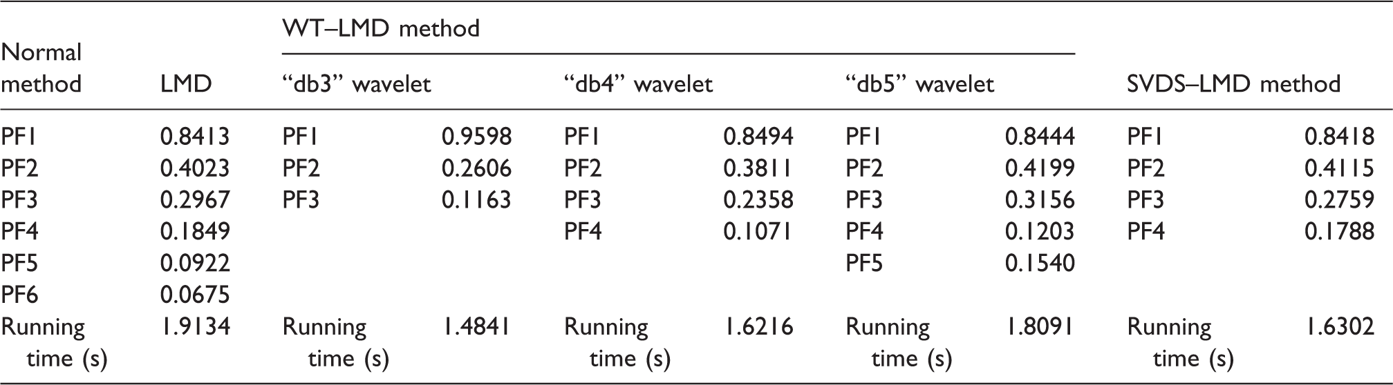
PF: product function; SVDS–LMD: singular value difference spectrum denoising and local mean decomposition; WT–LMD: wavelet denoising and local mean decomposition.

In order to demonstrate the necessity and effectiveness of SVDS denoising in the proposed method, the results of SVDS denoising are compared with WT denoising, which is widely used in denoising field. In the WT denoising method, the wavelet base functions “db3–db5” are commonly adopted to preprocess the noise in bearing fault diagnosis.^39,48–50 So, in follow-up WT denoising analysis, the “db3–db5” wavelet base functions will be used.

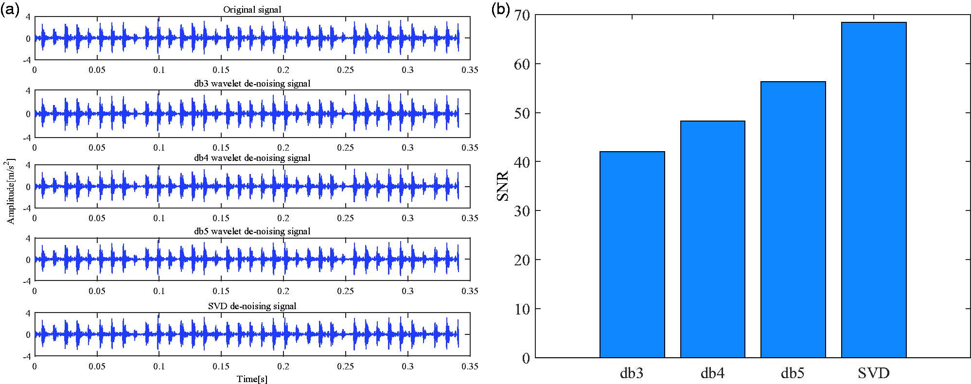
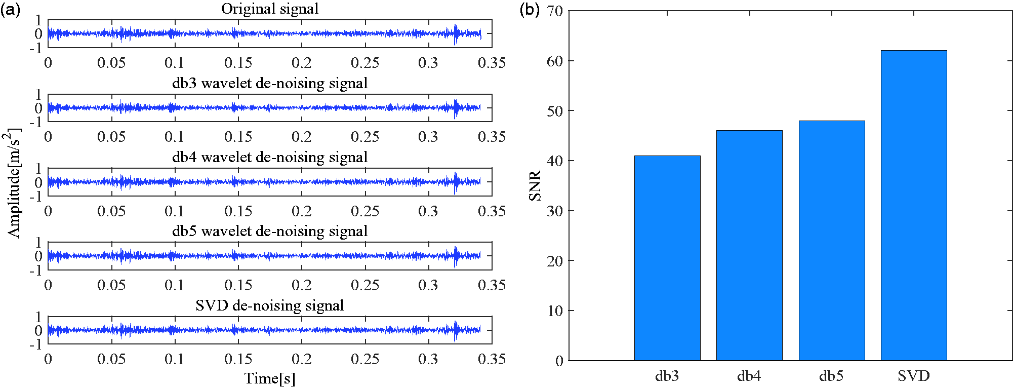
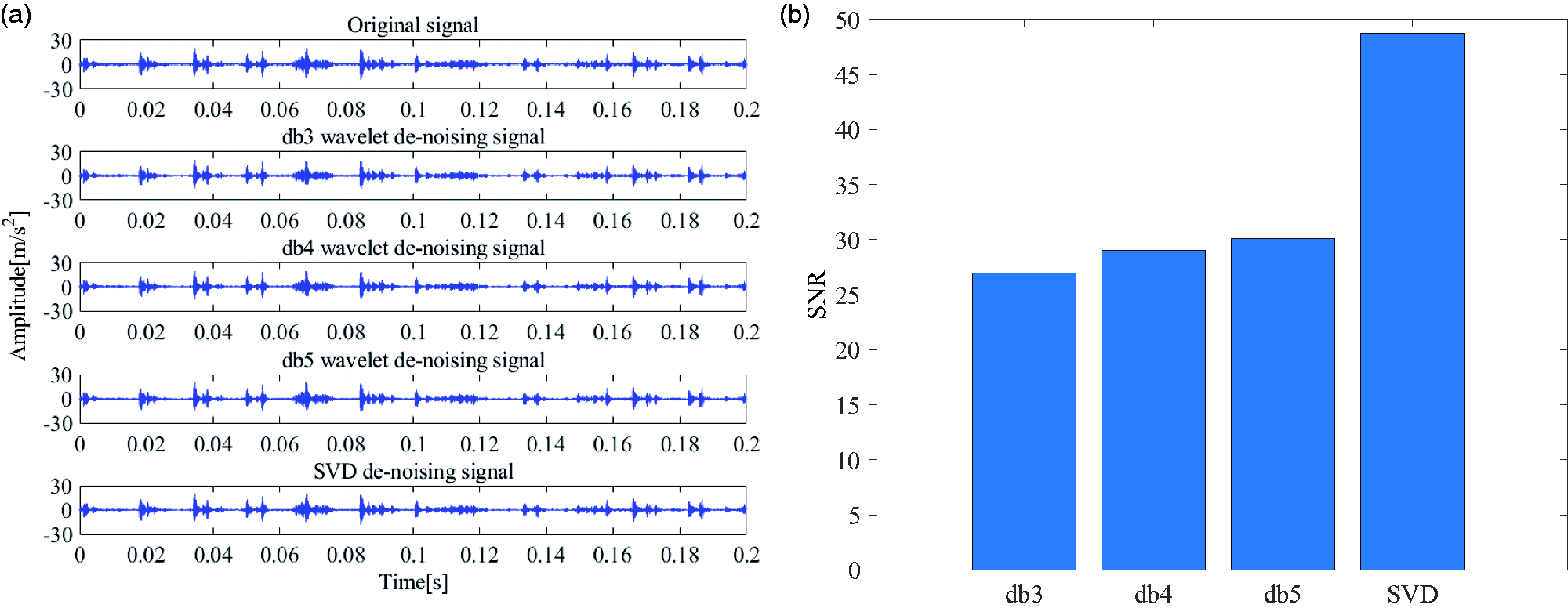
Figure 5 shows the denoising signal using the WT and SVDS method, respectively. As can be seen from Figure 5(a), the difference between two denoising methods cannot be seen directly from the denoised signal. Therefore, the SNR index is introduced to measure the merits of denoising methods and shown in Figure 5(b). In Figure 5(b), the SNR index shows that “db3–db5” wavelet can achieve similar effect in denoising. However, compared with the WT denoising method, the SVDS method achieves higher SNR.

Figure 5.

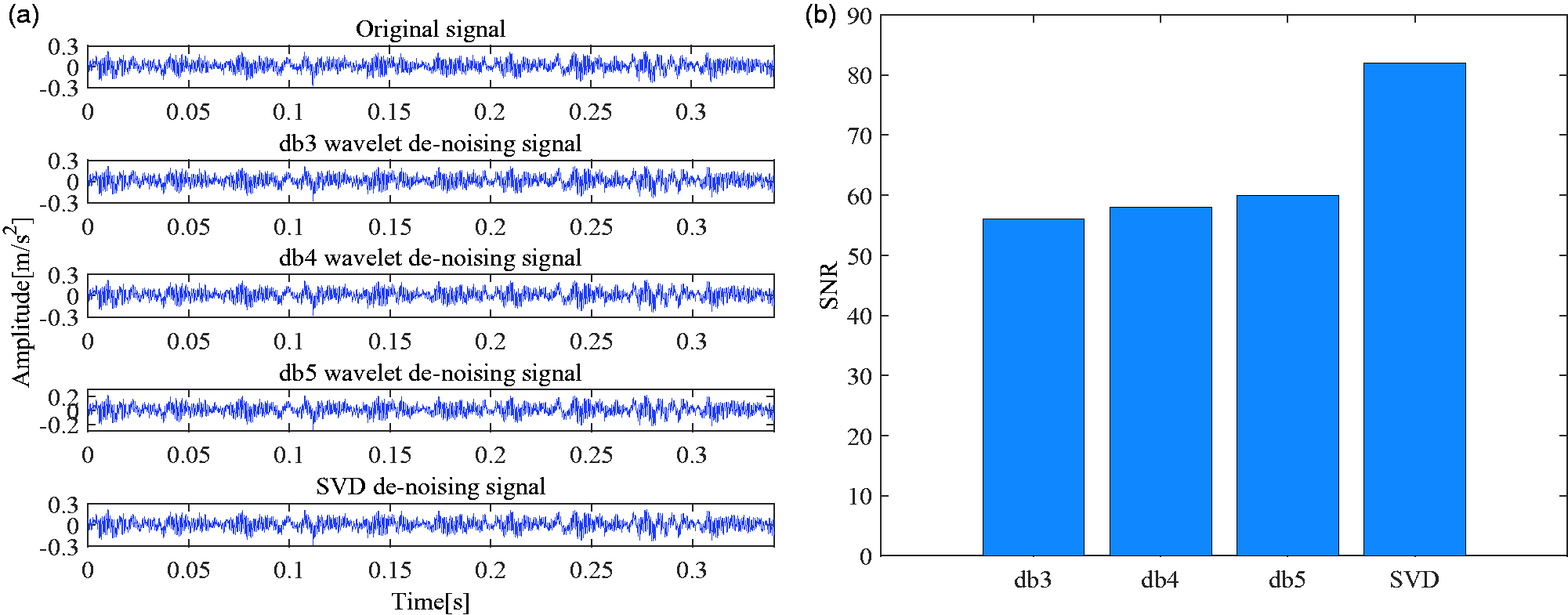
The denoising results. (a) Original signal and denoising signal and (b) SNR. SNR: signal-to-noise ratio.

In order to obtain more intuitive results, the denoised signals are decomposed by LMD, respectively, and the effective PF components are selected to calculate the Teager energy spectrum. Finally, the working state of the rolling bearing is distinguished according to the Teager energy spectrum.

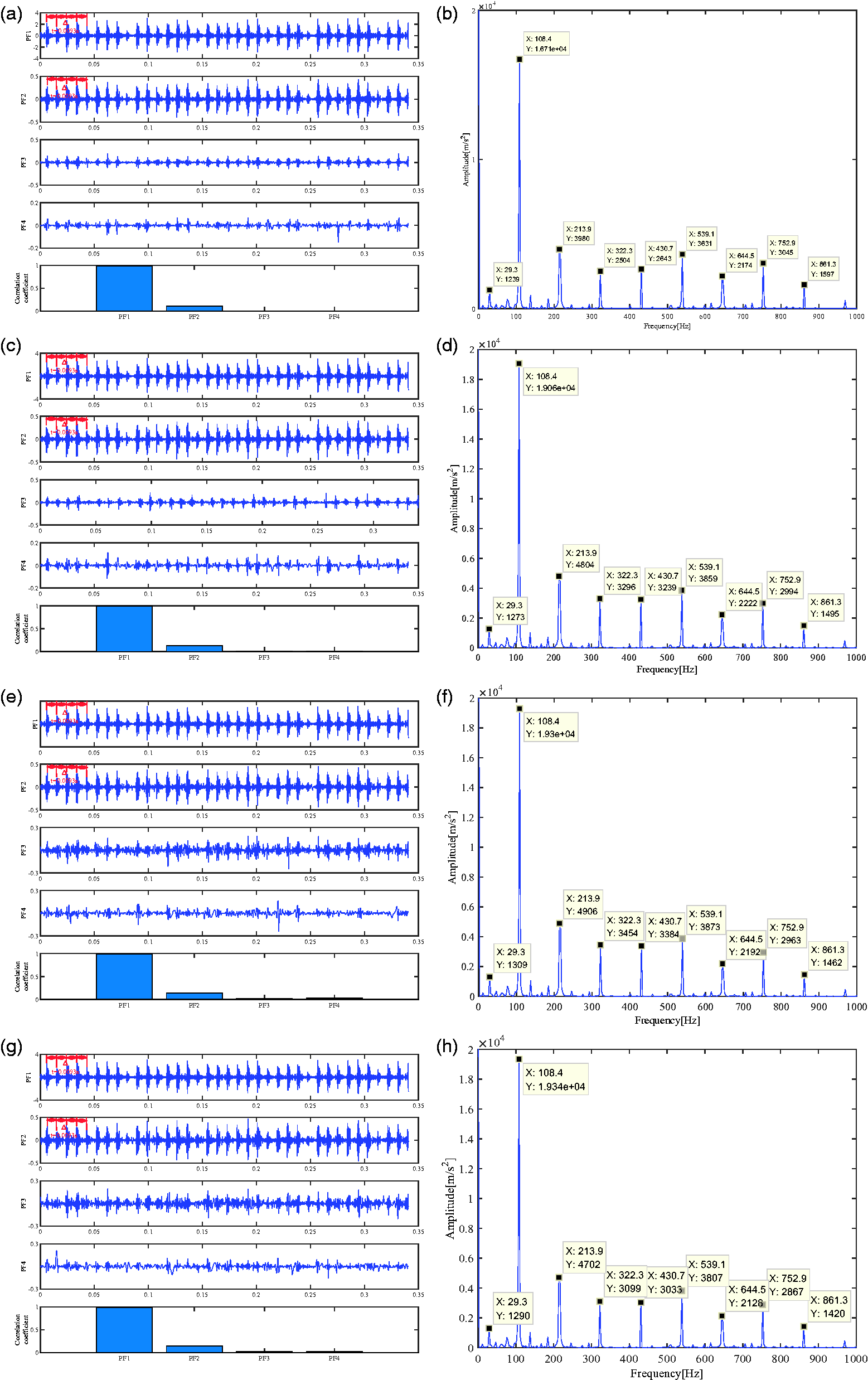
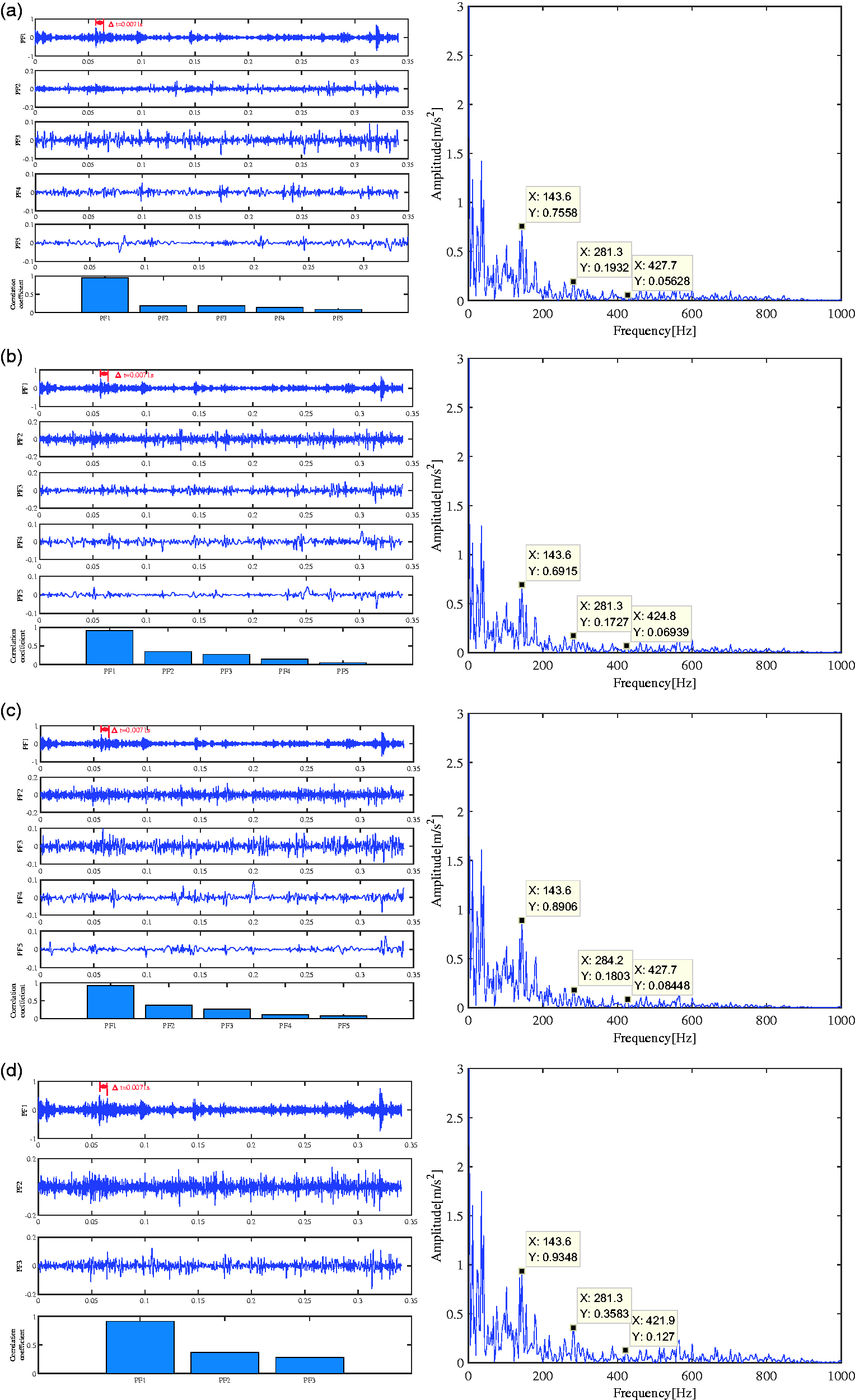
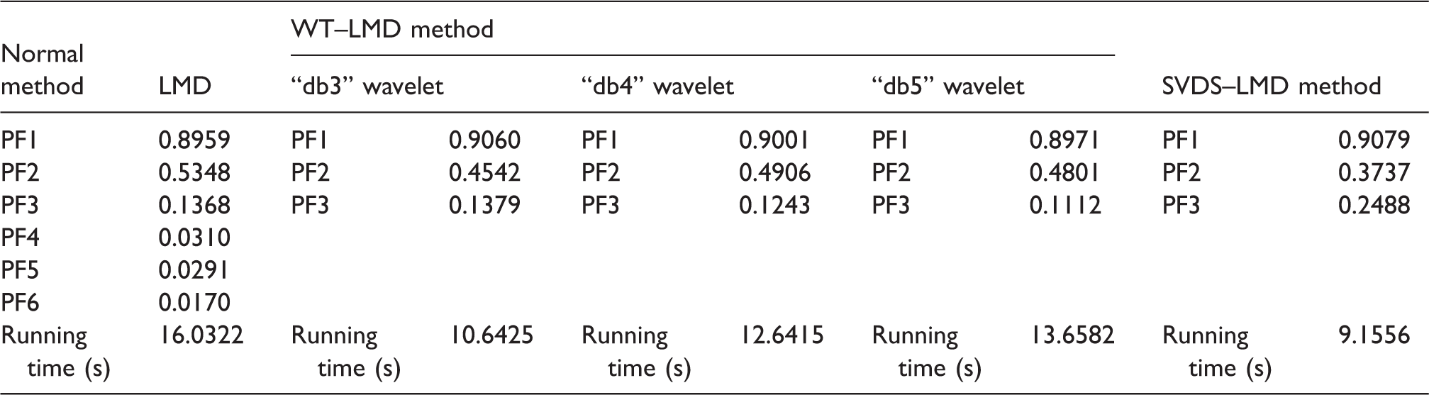
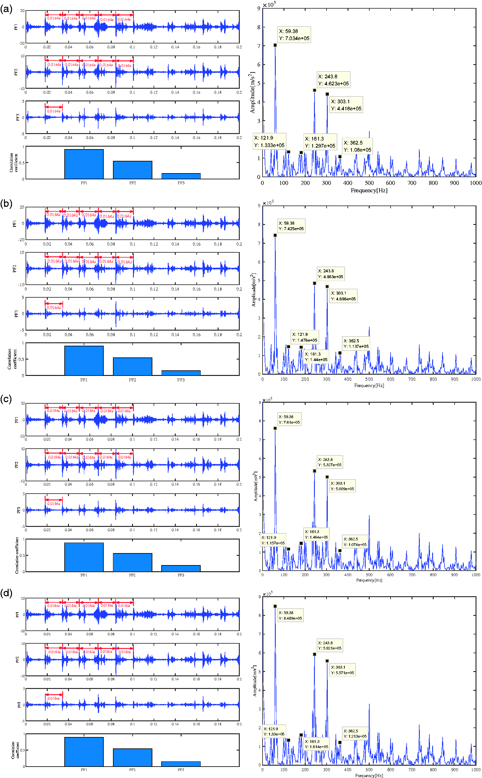
Figure 6 shows the experimental results obtained by WT–LMD and the proposed SVDS–LMD method. The result of correlation analysis is shown in Table 2, respectively. PF1 and PF2 are selected to reconstruct the follow-up signal x_new(t). We also can see that the periodical impulse of PF1 and PF2 is approximately equal to 0.034 s, which mainly corresponds to the rotating frequency (f_r=29.95 Hz) of the tested rolling bearing. The column on the right of Figure 6 shows the Teager energy spectrum of x_new(t) in several different methods. In Figure 6, it is easy to observe the rotating frequency f_r of the tested rolling bearing and its harmonics 2f_r. The results also show that when the bearing is in normal working condition, the above stated methods are quite effective. At the same time, by comparing the running time of the several methods, we can see that the presented SVDS–LMD method increases the denoising process, but it reduces the LMD decomposition loop iteration process. So, in terms of running time, the SVDS–LMD method is fairly or slightly less than the LMD and WT–LMD method (performed on a ThinkPad T450s at 2.19 GHz, using Matlab 2010b, the same below).

Figure 6.

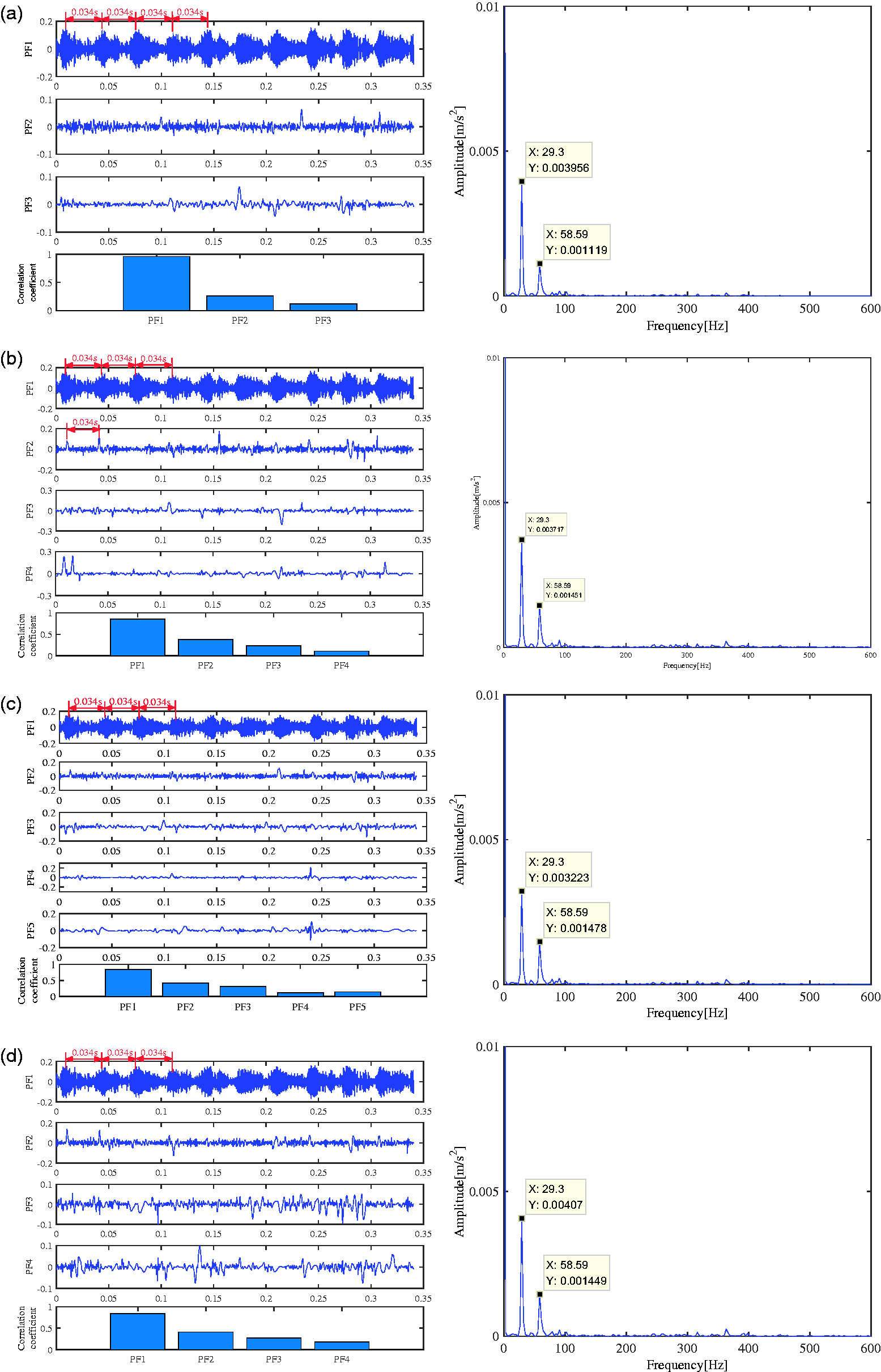
The experimental results of WT–LMD and SVDS–LMD methods. (a) The experimental results of WT–LMD in “db3” wavelet, (b) the experimental results of WT–LMD in “db4” wavelet, (c) the experimental results of WT–LMD in “db5” wavelet, and (d) the experimental results of SVDS–LMD.

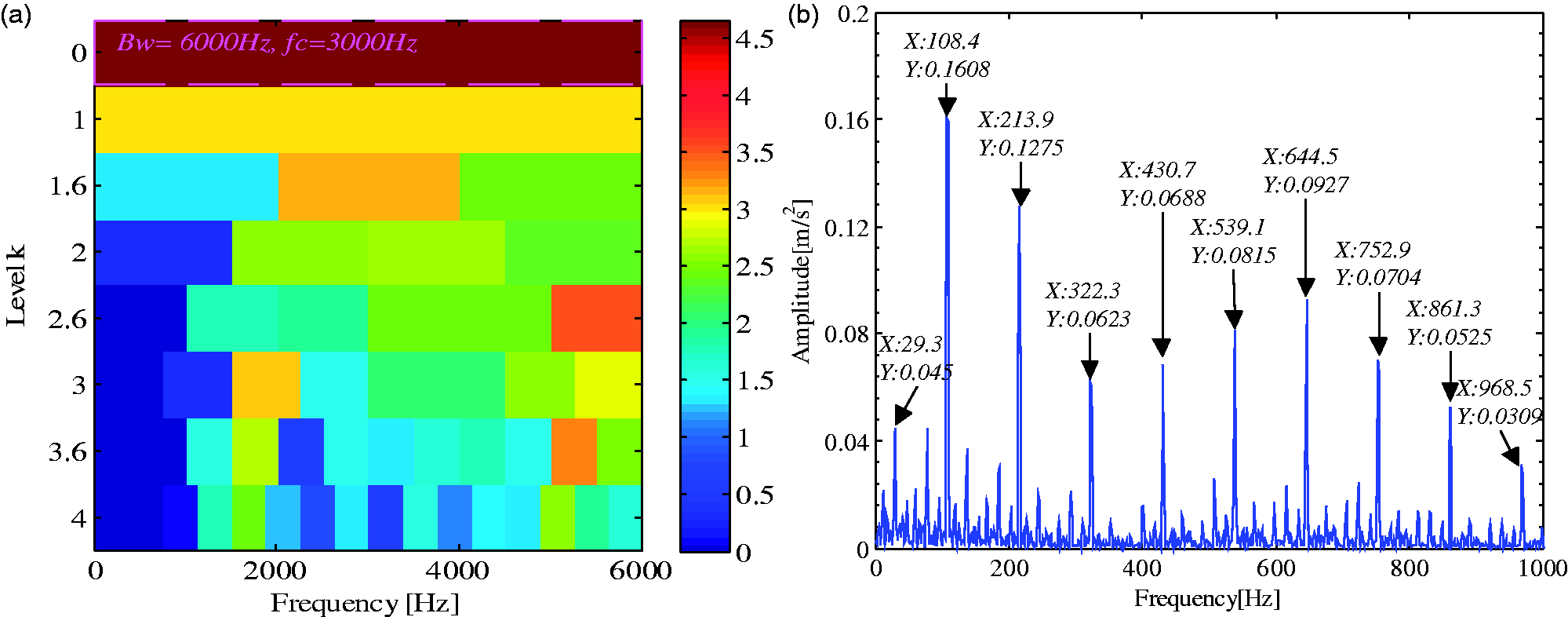
At the same time, we also use the FK as a demonstration to determine a prior wavelet parameter distribution because the FK attracts lots of attention in fault detection. The main idea of the FK is to use a metric called kurtosis to pick up a suitable band-pass filter with a center frequency fc and a bandwidth Bw from several band-pass filters with different center frequencies and bandwidths for detecting repetitive transients caused by bearing rolling element faults and gear faults. In the FK, it is assumed that the larger kurtosis is, the more a band-pass filter is informative for fault detection. The paving of the FK is plotted in Figure 7(a), where an optimal filter with the optimal center frequency of 1500 Hz and the bandwidth of 3000 Hz is found. In Figure 7(b), envelope spectrum of the signal obtained by the optimal filter provides healthy bearing without fault.

Figure 7.

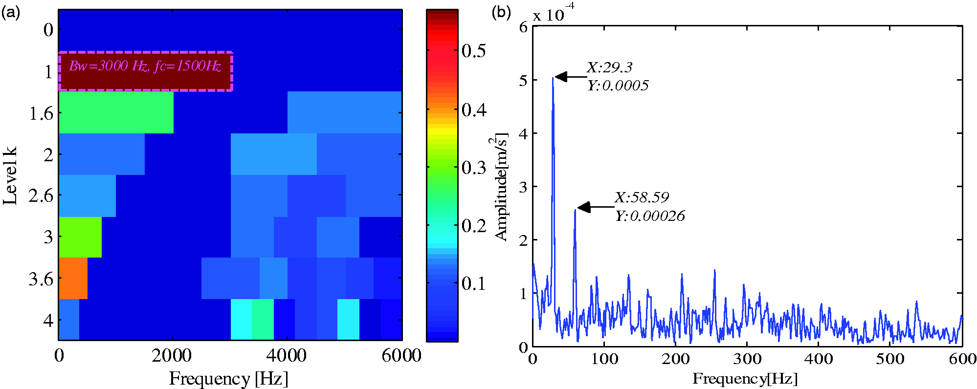
The results obtained by the FK for detecting normal bearing (the center frequency of 1500 Hz and the bandwidth of 3000 Hz). (a) The FK and (b) FFT spectrum. FFT: fast Fourier transform.

b. Inner ring fault

Figure 8 shows the temporal waveform and the FFT spectrum of the inner ring fault vibration signal collected from the tested bearing. Compared with Figure 3, the temporal waveform and the FFT spectrum have occurred the significant changes and added some abnormal frequency components in Figure 8. In the frequency spectrum of Figure 8(b), the BPFI can be detected. However, there are many interference frequency components with large amplitude in frequency spectrum in Figure 8(b). It greatly increases the difficulty of fault identification. So, the normal LMD, WT–LMD and the proposed SVDS–LMD method are applied to analyze this vibration signal, respectively.

Figure 8.

The time waveform and its corresponding FFT spectrum of the inner ring fault. (a) Time-domain waveform and (b) FFT spectrum. FFT: fast Fourier transform.

Figure 9(a) displays the first four PFs decomposed by the normal LMD method. And the correlation coefficients of the first two PFs are larger than 0.3. The periodical impulse in PF1 and PF2 is about 0.0062 seconds, which is roughly equal to BPFI = 162.19 Hz of the motor rolling bearing. Therefore, the first two PFs are selected to reconstruct the subsequent signal x_new(t). Figure 9(b) shows the Teager energy spectrum of x_new(t). In Figure 9(b), it can be seen that the fault feature frequency BPFI and its harmonics (2BPFI–6BPFI) along with the rotational frequency harmonics 2f_r can be observed. But, there are some interference frequency components with large amplitude. Therefore, in order to achieve better result, WT and SVDS denoising methods are introduced to perform signal denoising.

Figure 9.

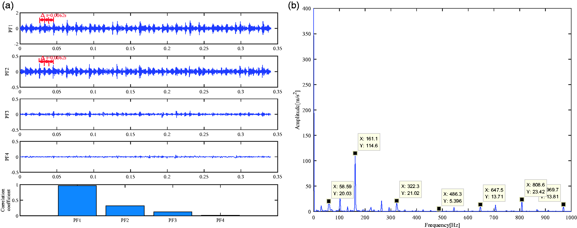
The analysis results of normal LMD method. (a) Decomposition results and (b) Teager energy spectrum.

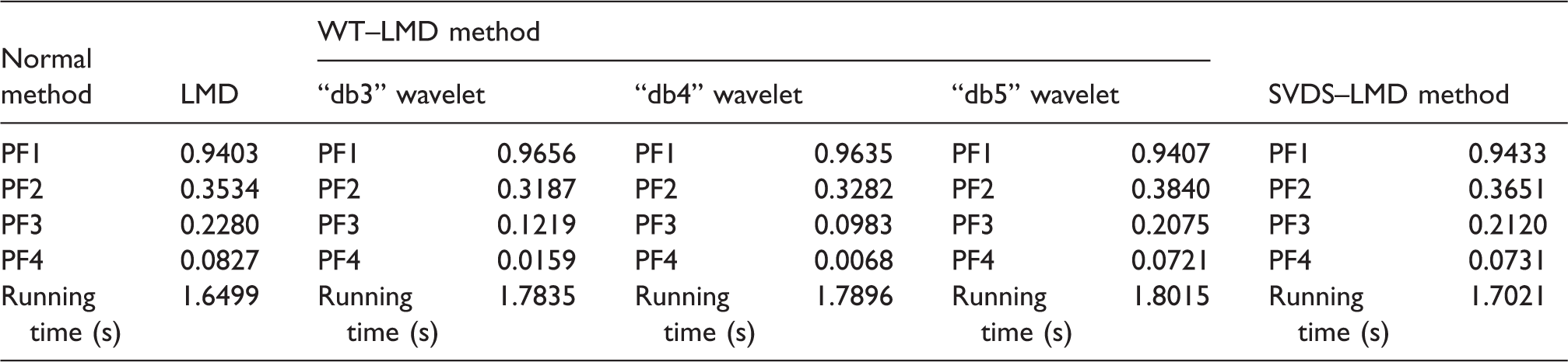
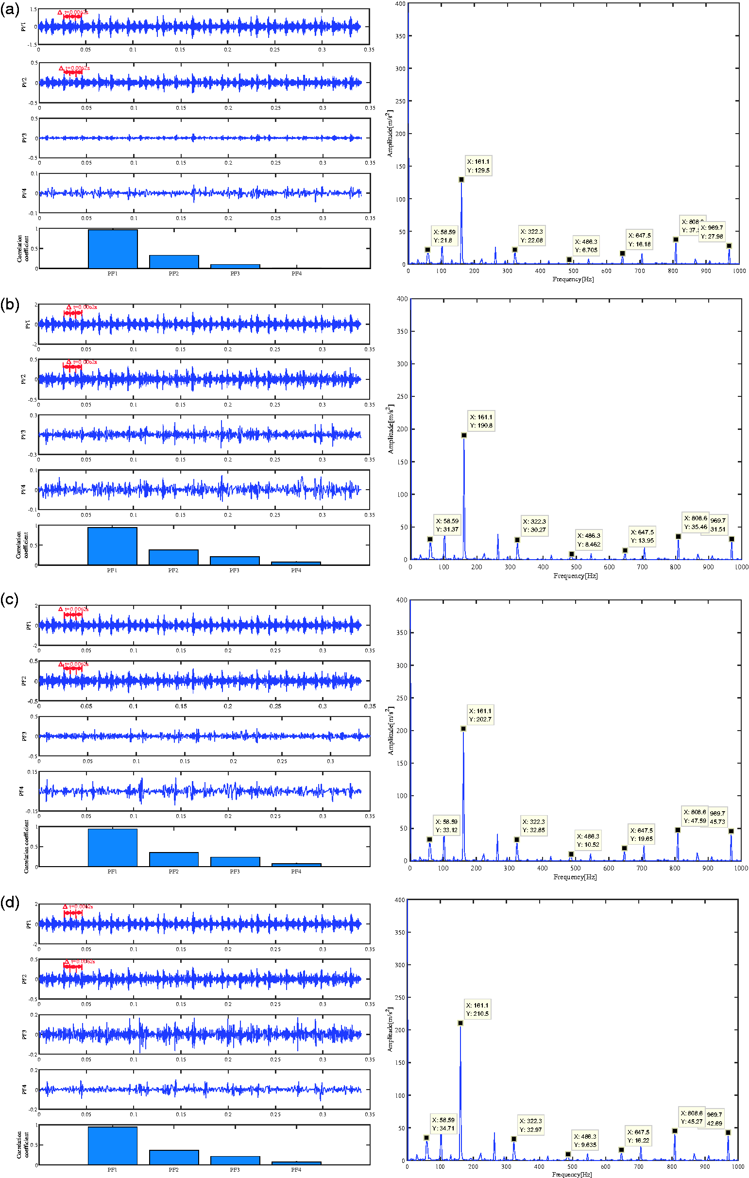
Figure 10 shows the denoising signal and SNR using the WT and SVDS methods, respectively, in inner ring fault. Comparing with the results of Figure 5, similar conclusions can be obtained. Figure 10 shows the experimental results of WT–LMD and the proposed SVDS–LMD method in inner ring fault. We also can see that the periodical impulse of PF1 and PF2 is approximately equal to 0.0062 seconds, which mainly corresponds to BPFI = 162.19 Hz of the tested rolling bearing. As shown in Table 3, PF1 and PF2 components are selected to reconstruct the subsequent signal x_new(t) according to the correlation coefficient criterion in WT–LMD and SVDS–LMD method. The column on the right of Figure 11 shows the Teager energy spectrum of x_new(t) in several different methods. It is easy to observe the inner ring defect frequency BPFI and its harmonics (2BPFI–6BPFI) along with the rotational frequency harmonics 2f_r. At the same time, through the comparative analysis of Teager energy spectrum in Figures 9 and 11, we can draw the following conclusions: (1) The WT and SVDS denoising method can enhance and highlight the fault characteristics of signal. (2) In “db3–db5” wavelet base functions, the denoising and spectrum analysis effect are getting better and better. Due to space constraints, the thesis cannot iterate over all wavelet base functions. Although “db5” wavelet is the wavelet base function widely used in bearing fault diagnosis and applied to obtain the better results in this paper, it may not be the best wavelet base function. (3) Compared to the WT denoising method, the SVDS denoising method is easy to implement and can achieve slightly better or equivalent processing effect than the WT denoising method. Moreover, in the case of the same number of LMD decomposition layers, the denoising process slightly increases the running time of the algorithm in WT–LMD and SVDS–LMD. But, the running time of SVD denoising process is less than WT denoising.

Figure 10.

The denoising results. (a) Original signal and denoising signal and (b) SNR. SNR: signal-to-noise ratio.

Table 3.

The correlation coefficients of PFs and the original vibration signal x(t).

Normal method	LMD	WT–LMD method
Normal method	LMD	“db3” wavelet		“db4” wavelet		“db5” wavelet		SVDS–LMD method
PF1	0.9403	PF1	0.9656	PF1	0.9635	PF1	0.9407	PF1	0.9433
PF2	0.3534	PF2	0.3187	PF2	0.3282	PF2	0.3840	PF2	0.3651
PF3	0.2280	PF3	0.1219	PF3	0.0983	PF3	0.2075	PF3	0.2120
PF4	0.0827	PF4	0.0159	PF4	0.0068	PF4	0.0721	PF4	0.0731
Running time (s)	1.6499	Running time (s)	1.7835	Running time (s)	1.7896	Running time (s)	1.8015	Running time (s)	1.7021

PF: product function; SVDS–LMD: singular value difference spectrum denoising and local mean decomposition; WT–LMD: wavelet denoising and local mean decomposition.

Figure 11.

The experimental results of WT–LMD and SVDS–LMD methods (inner ring fault). (a) The experimental results of WT–LMD in “db3” wavelet, (b) the experimental results of WT–LMD in “db4” wavelet, (c) the experimental results of WT–LMD in “db5” wavelet, and (d) the experimental results of SVDS–LMD.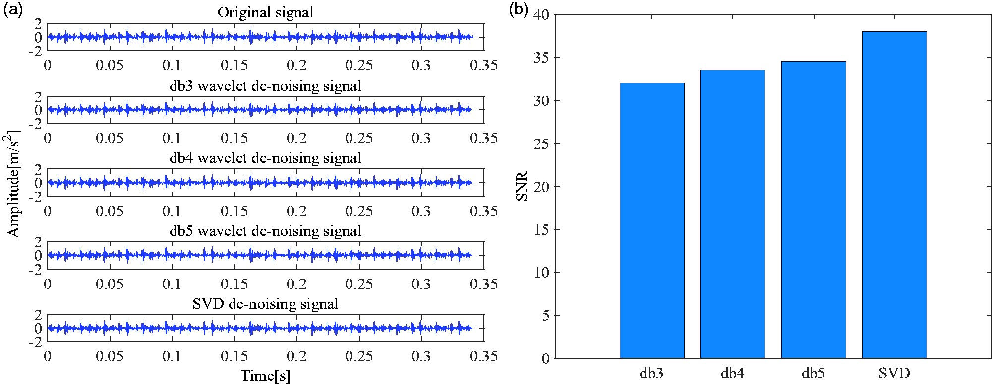

For further comparison, the FK is applied to the same outer race fault signal shown in Figure 12(a). In Figure 12(b), envelope spectrum of the signal obtained by the optimal filter provides inner race fault signatures for bearing fault diagnosis. The inner race fault-related signatures can be also identified by inspecting the inner race fault characteristic frequency and its harmonics. However, compared with the proposed method, the frequency spectra obtained by the FK contain heavy noise which corrupts the visual inspection ability.

Figure 12.

The results obtained by the FK for detecting an inner race fault (the center frequency of 3000 Hz and the bandwidth of 6000 Hz). (a) The FK and (b) FFT spectrum. FFT: fast Fourier transform.

c. Outer ring fault

Figure 13 shows the temporal waveform and the FFT spectrum of the outer ring fault vibration signal collected from the tested bearing. It can be seen that the bearing fault has occurred . But the fault impulse features are buried in the background noise and difficult to be identified in Figure 13. So, the normal LMD, WT–LMD and the proposed SVDS–LMD method are applied to analyze this vibration signal, respectively.

Figure 13.

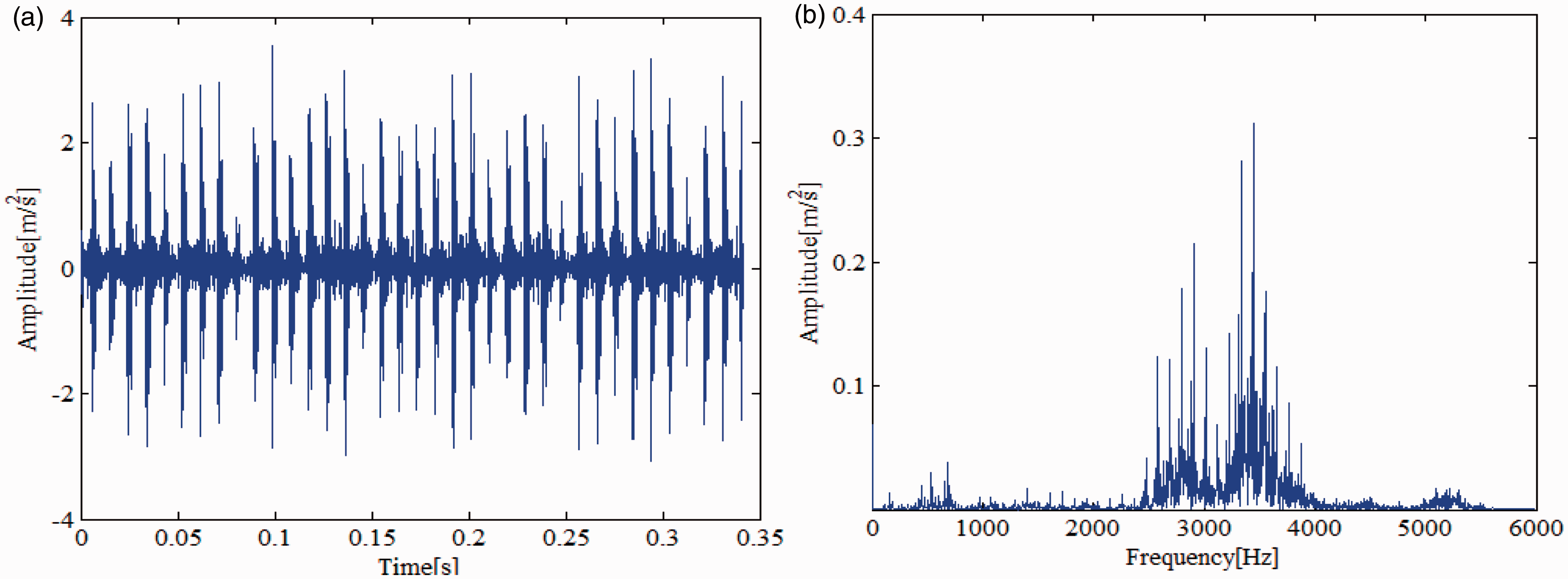
The time waveform and its corresponding FFT spectrum of the outer ring fault. (a) Time-domain waveform and (b) FFT spectrum. FFT: fast Fourier transform.

Figure 14(a) displays the first six PFs obtained by the normal LMD method. In order to eliminate the false components in the decomposition process, the correlation coefficients of PFs are calculated and shown in Table 4. It can be observed that the correlation coefficient of the PF1 is larger than 0.3. The periodical impulse in PF1 is about 0.0093 seconds, which is approximately equal to the BPFO = 107.36 Hz of the motor rolling bearing. Therefore, the PF1 is selected to reconstruct the new and subsequent analysis signal x_new(t). Figure 14(b) shows the Teager energy spectrum of x_new(t). It can be seen that the fault feature frequency BPFO and its harmonics (2BPFO–8BPFO), along with the rotating frequency f_r can be clearly observed in Figure 14(b).

Figure 14.

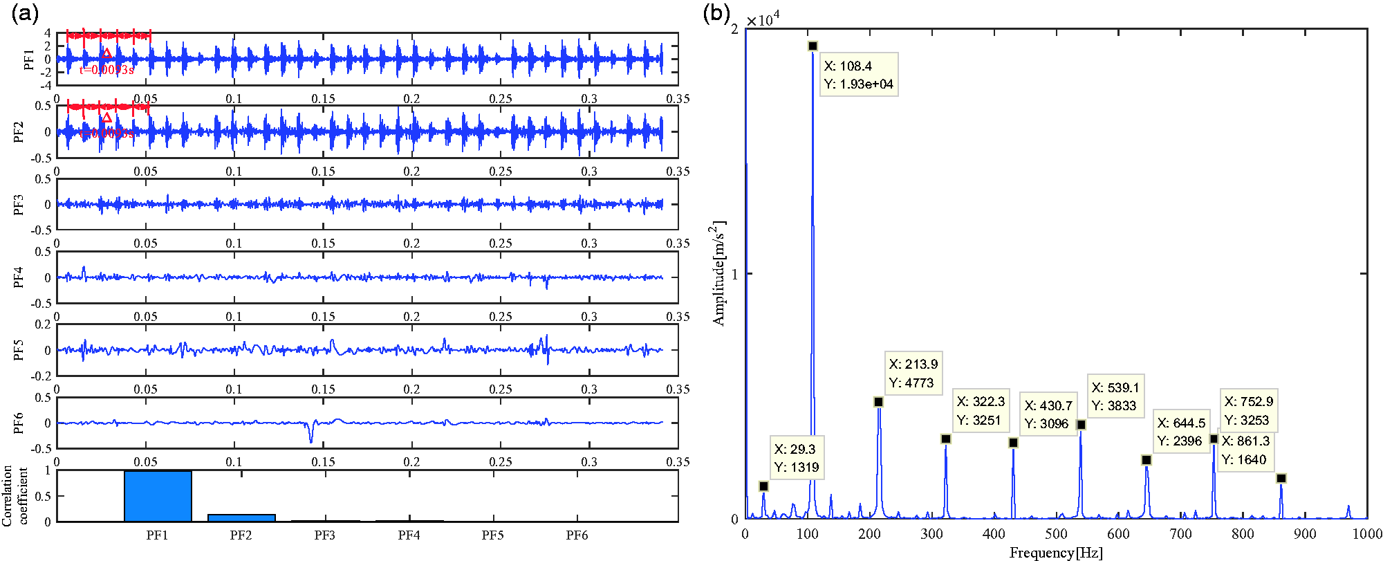
The analysis results of normal LMD method. (a) Decomposition results and (b) Teager energy spectrum.

Table 4.

The correlation coefficients of PFs and the original vibration signal x(t).

Normal method	LMD	WT–LMD method
Normal method	LMD	“db3” wavelet		“db4” wavelet		“db5” wavelet		SVDS–LMD method
PF1	0.9871	PF1	0.9898	PF1	0.9880	PF1	0.9887	PF1	0.9873
PF2	0.1418	PF2	0.1261	PF2	0.1377	PF2	0.1374	PF2	0.1381
PF3	0.0221	PF3	0.0029	PF3	0.0191	PF3	0.0006	PF3	0.0197
PF4	0.0251	PF4	0.0032	PF4	0.0287	PF4	0.0101	PF4	0.0213
PF5	0.0117
PF6	0.0009
Running time (s)	1.6133	Running time (s)	1.7036	Running time (s)	1.7393	Running time (s)	1.7434	Running time (s)	1.6294

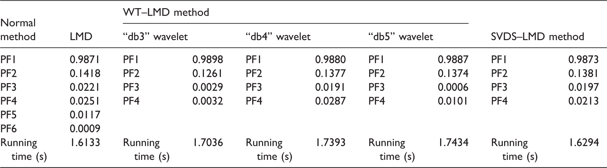
PF: product function; SVDS–LMD: singular value difference spectrum denoising and local mean decomposition; WT–LMD: wavelet denoising and local mean decomposition.

In order to highlight the fault characteristics and suppress the interference components, WT and SVDS denoising methods are introduced to perform signal denoising in Figure 15. As can be seen from Figure 15, the SVD denoising effect is better than WT denoising. Figure 16 displays the experimental results obtained by WT–LMD and the proposed SVDS–LMD method in outer ring fault. We also can see that the periodical impulse of PF1 is approximately equal to 0.0093 s, which mainly corresponds to BPFO = 107.36 Hz of the tested rolling bearing. As shown in Table 4, PF1 components are selected to reconstruct the subsequent signal x_new(t) according to the correlation coefficient criterion in WT–LMD and SVDS–LMD methods. The column on the right of Figure 16 shows the Teager energy spectrum of x_new(t) in several different methods. It is easy to observe the outer ring defect frequency BPFO and its harmonics (2BPFO–8BPFO) along with the rotational frequency harmonics f_r. At the same time, through the comparative analysis of Teager energy spectrum, the similar conclusions with inner ring fault can be obtained.

Figure 15.

The denoising results. (a) Original signal and denoising signal and (b) SNR. SNR: signal-to-noise ratio.

Figure 16.

The experimental results of WT–LMD and SVDS–LMD methods (outer ring fault). (a) The experimental results of WT–LMD in “db3” wavelet, (b) the experimental results of WT–LMD in “db4” wavelet, (c) the experimental results of WT–LMD in “db5” wavelet, and (d) the experimental results of SVDS–LMD.

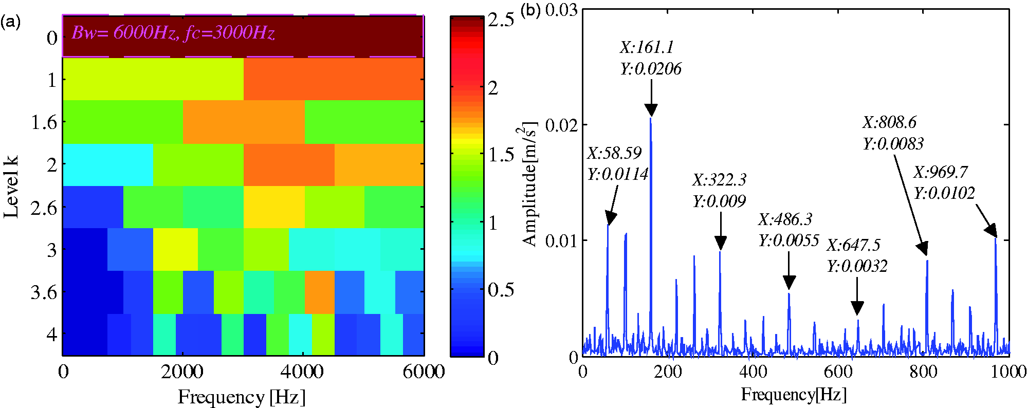
Similarly, the paving of the FK is plotted in Figure 17(a), where an optimal filter with the optimal center frequency of 3000 Hz and the bandwidth of 6000 Hz is found. In Figure 17(b), envelope spectrum of the signal obtained by the optimal filter provides outer race fault signatures for bearing fault diagnosis. And then, some similar conclusions with the inner race fault can be obtained.

Figure 17.

The results obtained by the FK for detecting an outer race fault (the center frequency of 3000 Hz and the bandwidth of 6000 Hz). (a) The FK and (b) FFT spectrum. FFT: fast Fourier transform.

d. Rolling element fault

Figure 18 shows the temporal waveform and the FFT spectrum of the rolling element fault vibration signal collected from the tested bearing. It can be seen that the bearing fault has occurred. Compared with inner ring fault and outer ring fault vibration signal, the fault vibration signal of rolling element is more complex. At the same time, the impulse features are buried in the background noise and difficult to be identified. So, the normal LMD, WT–LMD and the proposed SVDS–LMD methods are applied to analyze this vibration signal, respectively.

Figure 18.

The time waveform and its corresponding FFT spectrum of the rolling element fault. (a) Time-domain waveform and (b) FFT spectrum. FFT: fast Fourier transform.

Figure 19(a) displays the first six PFs obtained by the normal LMD method. The correlation coefficients of PFs are calculated and shown in Table 5. It can be observed that the correlation coefficients of the first two PFs are larger than 0.3. The periodical impulse in PF1 is about 0.0071 seconds, which is approximately equal to the fault characteristic frequency (BSF = 141.7 Hz) of the motor rolling bearing. Therefore, the PF1 and PF2 are selected as the fault feature signal to obtain the reconstruction signal x_new(t). Figure 19(b) shows the Teager energy spectrum of x_new(t). In Teager energy spectrum, it can be seen that the fault feature frequency BSF and its harmonics (2BSF–3BSF) can be observed, but along with some strong interference frequency components.

Figure 19.

The analysis results of normal LMD method. (a) Decomposition results and (b) Teager energy spectrum.

Table 5.

The correlation coefficients of PFs and the original vibration signal x(t).

Normal method	LMD	WT–LMD method
Normal method	LMD	“db3” wavelet		“db4” wavelet		“db5” wavelet		SVDS–LMD method
PF1	0.9082	PF1	0.9169	PF1	0.9186	PF1	0.9119	PF1	0.9079
PF2	0.3739	PF2	0.3505	PF2	0.3790	PF2	0.3704	PF2	0.3737
PF3	0.2734	PF3	0.2742	PF3	0.2612	PF3	0.2816	PF3	0.2488
PF4	0.1570	PF4	0.1429	PF4	0.1181	PF4	0.1588
PF5	0.0960	PF5	0.0484	PF5	0.0790	PF5	0.0810
PF6	0.0522
PF7	0.0196
Running time (s)	2.2709	Running time (s)	1.6146	Running time (s)	1.6187	Running time (s)	1.7323	Running time (s)	1.5150

PF: product function; SVDS–LMD: singular value difference spectrum denoising and local mean decomposition; WT–LMD: wavelet denoising and local mean decomposition.

In order to highlight the fault characteristics and suppress the interference components, WT and SVDS denoising methods are introduced to perform signal denoising. Figure 20 shows the denoising signal and SNR using the WT and SVDS methods, respectively. The above-mentioned denoising signal is analyzed by WT–LMD and the proposed SVDS–LMD and shown in Figure 21.

Figure 20.

The denoising results. (a) Original signal and denoising signal and (b) SNR. SNR: signal-to-noise ratio.

Figure 21.

The experimental results of WT–LMD and SVDS–LMD methods (rolling element fault). (a) The experimental results of WT–LMD in “db3” wavelet, (b) the experimental results of WT–LMD in “db4” wavelet, (c) the experimental results of WT–LMD in “db5” wavelet, and (d) the experimental results of SVDS–LMD.

As shown in Figure 21(a) to (c), the first five PFs are obtained by the WT–LMD method. It can be observed that the correlation coefficients of the first two PFs are larger than 0.3. The periodical impulse in PF1 is about 0.0072 seconds, which is approximately equal to the fault characteristic frequency (BSF = 141.7 Hz) of the motor rolling bearing. Therefore, the PF1 and PF2 are selected to reconstruct signal x_new(t). Then, Teager energy spectrum of x_new(t) is calculated and shown in the right column of Figure 21. It can be seen that the fault feature frequency BSF and its harmonics (2BSF–3BSF) can be observed. Figure 21(d) shows the experimental result of the proposed SVDS–LMD method. Compared with the Teager energy spectrum of the normal LMD and WT–LMD in Figures 19 and 21(a) to (c), the proposed SVDS–LMD highlights the fault characteristics and improves the accuracy in fault diagnosis. At the same time, the proposed SVD–LMD method has higher SNR and faster running speed than normal LMD method and WT–LMD.

The FK is applied to the same outer race fault signal shown in Figure 22(a). In Figure 22(b), envelope spectrum of the signal obtained by the optimal filter provides rolling element fault signatures for bearing fault diagnosis. Although the above-mentioned methods can detect the rolling element localized faults, the frequency spectrums obtained by these methods are not totally ideal. However, comparatively speaking, the frequency spectrum obtained by the proposed method provides the best visual inspection ability for rolling element localized fault diagnosis.

Figure 22.

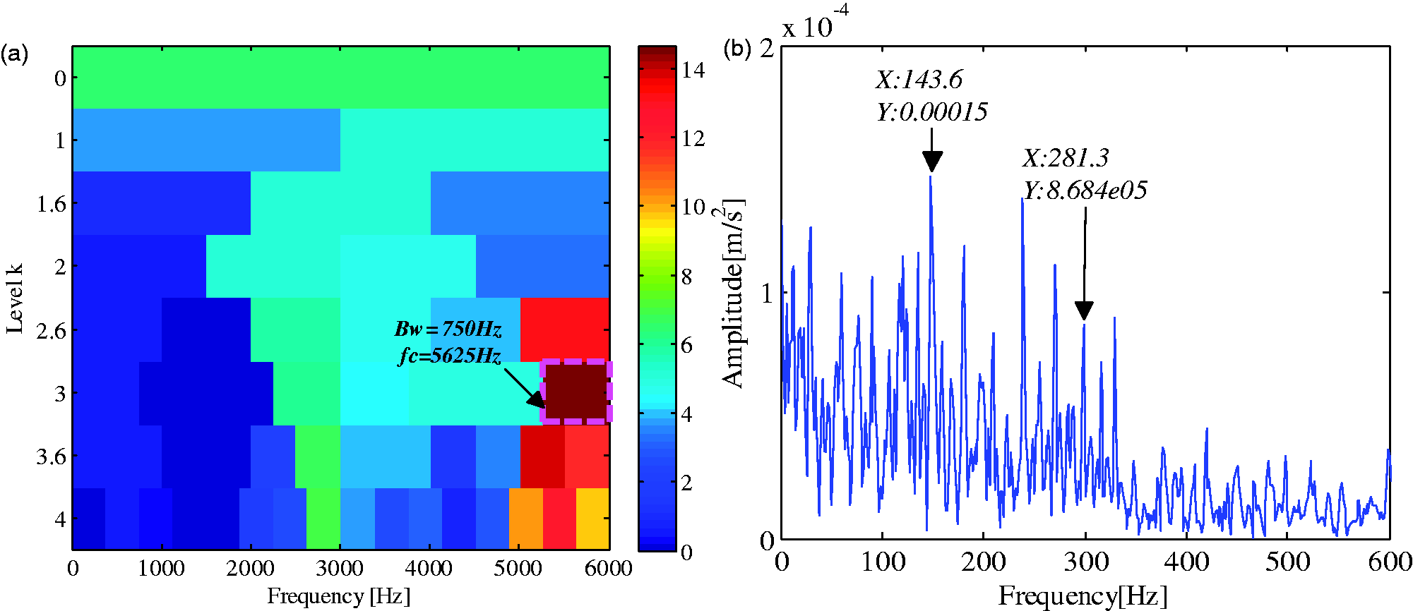
The results obtained by the FK for detecting a rolling element fault (the center frequency of 5625 Hz and the bandwidth of 750 Hz). (a) The FK and (b) FFT spectrum. FFT: fast Fourier transform.

Engineering application

In the past section, the effectiveness of the proposed method is verified by using experimental data sets of the rolling bearing which come from CWRU. To further prove the validity of the proposed method, the practical test data acquired by the rotor experiment platform are selected for subsequent analysis.

Data acquisition

The experimental device is shown in Figure 23. The device consists of three PCB acceleration sensors: four-channel dynamic data collecting card (NIUSB-9234), PC, and QPZZ-II rotating machinery vibration analysis and fault experiment system. The outer ring fault of rolling bearing is simulated in this experiment. The bearing parameters are elaborated in Table 6.

Figure 23.

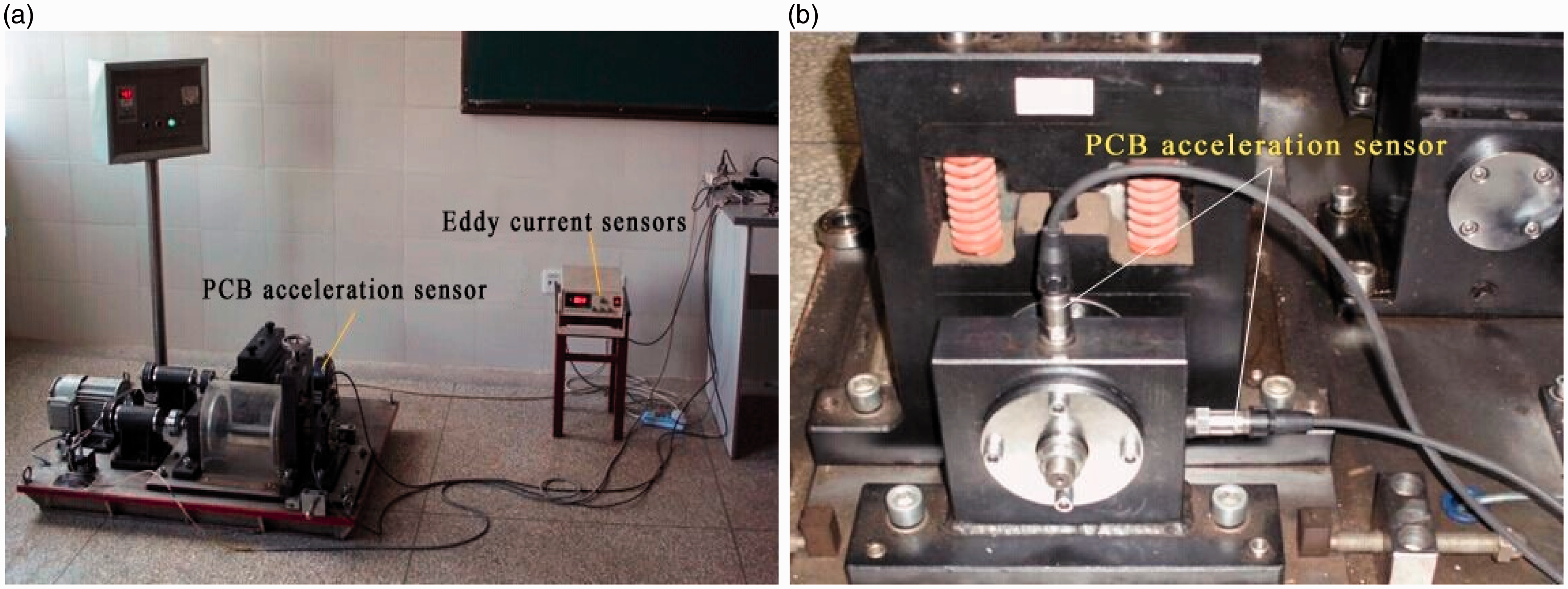
The experimental facilities. (a) The experimental structure and (b) the installation location of the PCB sensor. PCB Piezotronics, Inc.: ▪.

Table 6.

The N205EM bearing parameter.

Rolling element number (Z)	Contact angle (θ)	Rolling element diameter d (mm)	Pitch diameter D (mm)	Rotational speed (r/min)
12	0°	7.5	39	740

Combining the theoretical calculation formula equation (8) of BPFO with bearing parameters shown in Table 6, the rolling bearing fault characteristic frequency (BPFO = 59.75 Hz) is calculated. In this experiment, the sample frequency f_s of the vibration signals is 102,400 Hz and the data length N is 20,480.

Results and analysis

The time-domain and frequency-domain waveform of the vibration signal are shown in Figure 24. In Figure 24, there exists obvious impact components in the high frequency part. The bearing can be judged to be abnormal, but the relevant information of failure cannot be obtained. Therefore, the normal LMD, WT–LMD and the proposed SVDS–LMD method are introduced to finish further analysis.

Figure 24.

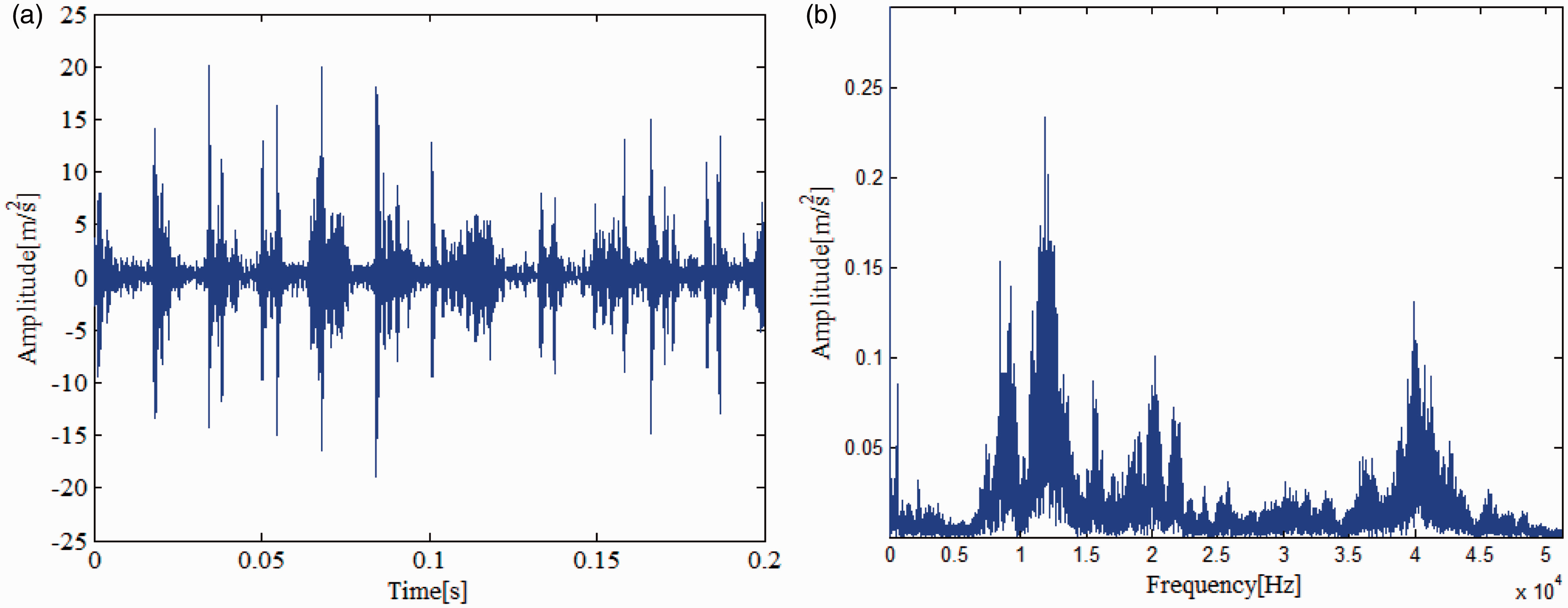
The time waveform and its corresponding FFT spectrum of the rolling element fault. (a) Time-domain waveform and (b) FFT spectrum. FFT: fast Fourier transform.

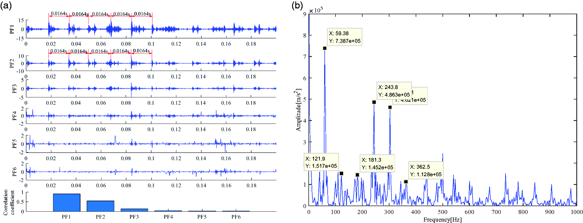
Figure 25 shows the results of the normal LMD method. Because the first six PFs have contained almost all fault information, other PFs and residual are omitted. Moreover, the correlation coefficients are calculated through equation (5) and shown in Table 7. The correlation coefficients of PF1 and PF2 are greater than 0.3. Therefore, the PF1 and PF2 are selected to calculate the reconstruction signal x_new(t). Figure 25(b) shows the Teager energy spectrum of x_new(t). In Figure 25(b), it can be seen that the fault characteristic frequency BPFO and its harmonics (2BPFO–5BPFO) can be identified. In order to highlight the fault characteristics and suppress the interference components, WT and SVDS denoising method are introduced to perform signal denoising. Figure 26 shows the denoised signal and SNR using the WT and SVDS methods, respectively. The above-mentioned denoising signal is analyzed by WT–LMD and the proposed SVDS–LMD and shown in Figure 27.

Figure 25.

The analysis results of normal LMD method. (a) Decomposition results and (b) Teager energy spectrum.

Table 7.

The correlation coefficients of PFs and the decomposition signal x(t).

Normal method	LMD	WT–LMD method
Normal method	LMD	“db3” wavelet		“db4” wavelet		“db5” wavelet		SVDS–LMD method
PF1	0.8959	PF1	0.9060	PF1	0.9001	PF1	0.8971	PF1	0.9079
PF2	0.5348	PF2	0.4542	PF2	0.4906	PF2	0.4801	PF2	0.3737
PF3	0.1368	PF3	0.1379	PF3	0.1243	PF3	0.1112	PF3	0.2488
PF4	0.0310
PF5	0.0291
PF6	0.0170
Running time (s)	16.0322	Running time (s)	10.6425	Running time (s)	12.6415	Running time (s)	13.6582	Running time (s)	9.1556

PF: product function; SVDS–LMD: singular value difference spectrum denoising and local mean decomposition; WT–LMD: wavelet denoising and local mean decomposition.

Figure 26.

The denoising results. (a) Original signal and denoising signal and (b) SNR. SNR: signal-to-noise ratio.

Figure 27.

As shown in Figure 26(a), the wavelet base function “db3–db5” and SVDS are adopted to preprocess the noise, but the difference of denoised results between different wavelet base functions and SVDS is not very obvious. As can be seen from the SNR index, the SVDS denoising method can achieve the better result.

In order to compare with the experimental results, further analysis of the above denoised signal is carried out, respectively. The results of the LMD decomposition and the demodulation of TEO for denoised signal are calculated to diagnose the fault of rolling bearing. The decomposition results of LMD and Teager energy spectrum of the effective PF components through denoising of WT and SVDS are shown in Figure 27.

The LMD decomposition results of the signal through different wavelet base functions are shown in Figure 27(a) to (c). And the correlation coefficients between the PF components decomposed by LMD are calculated and shown in Table 7. As shown in Table 7, the PF1 and PF2 components will be selected as valid components for subsequent analysis so as to obtain Teager energy spectrum in the right column of Figure 27. It can be seen by energy spectrum in Figure 27(a) to (c) that the final Teager energy spectrum is more clearer when using the wavelet base function db5. Figure 27(d) displays the decomposition results of the proposed SVDS–LMD method and Teager energy spectrum. The PF1 and PF2, whose correlation coefficient is larger than 0.3, are selected to reconstruct the subsequent analysis signal x_new(t). In Figure 27(d), it can be seen that the fault characteristic frequency BPFO and its harmonics (2BPFO–5BPFO) can be clearly identified in Teager energy spectrum of x_new(t). However, compared with the proposed method in this paper, the result of db5 wavelet base function is not the optimal result. Therefore, it is necessary to combine the characteristics of actual signal to analyze in depth and decide how to choose the proper wavelet base function to achieve better effect. This will inevitably lead to the sharp increasing of complexity and operational difficulty. On the contrary, the proposed SVDS–LMD method in this paper is more simple and easy to operate and has good effect on noise suppression and great application value in engineering as well.

In the actual test, the FK is applied to the same outer race fault signal shown in Figure 28(a). In Figure 28(b), envelope spectrum of the signal obtained by the optimal filter provides inner race fault signatures for bearing fault diagnosis. From the result shown in Figure 24(b), bearing outer race fault-related signatures are also identified by inspecting the outer race fault characteristic frequency and its harmonics. In the case of outer race fault diagnosis, although the above-mentioned methods are effective in detecting the outer race localized faults, frequency spectrum obtained by the proposed method is clearest to show outer race fault characteristic frequency and its harmonics. Frequency spectra obtained by the other methods contain heavy noise which corrupts the visual inspection ability.

Figure 28.

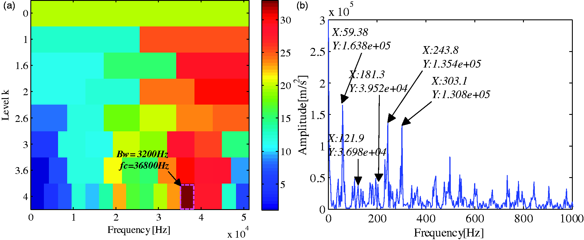
The results obtained by the FK for detecting an outer race fault (the center frequency of 36,800 Hz and the bandwidth of 3200 Hz). (a) The FK and (b) FFT spectrum. FFT: fast Fourier transform.

Conclusion

In this paper, the SVDS, LMD and TEO are combined as a hybrid method for fault diagnosis of rolling bearing.

The experimental results demonstrate the superiority of the proposed method. Some conclusions are summarized as follows:

The denoising method of SVDS is introduced to eliminate the noising of original vibration signal. It can filter out the high-frequency disturbance and enhance the energy of the low-frequency feature signal. To verify the effectiveness of the proposed denoise method, the original signal and the filtered signal are further decomposed by the LMD method and the false components of LMD are eliminated based on correlation analysis. The experimental results demonstrate that the proposed SVDS–LMD method has better performance on the improvement of the SNR, which greatly increases the computing efficiency. Furthermore, it is helpful on the improvement of performance and accuracy of the LMD.

The difficult problems of choosing the proper wavelet base function in WT can be solved by the proposed SVDS–LMD method. The denoising process can be adaptively finished according to the SVDS. In addition, considering that the following LMD method can remove part of noise, so that the results obtained by applying the LMD show clear characteristic frequencies can be identified by Teager energy spectrum.

Footnotes

Declaration of conflicting interests

The author(s) declared no potential conflicts of interest with respect to the research, authorship, and/or publication of this article.

Funding

The author(s) disclosed receipt of the following financial support for the research, authorship, and/or publication of this article: This work is supported by the National Natural Science Foundation of China (No. 51169007, 51765022 and 61663017) and Science & Research Program of Yunnan Province (No. 2015ZC005).

References

Henríquez

Alonso

Ferrer

et al . Application of the Teager-Kaiser energy operator in bearing fault diagnosis. ISA Trans 2013; 52: 278–284.

Peng

Yang

et al . Mixed-domain feature extraction approach to rolling bearings faults based on kernel principle component analysis. J Central South Univ (Sci Technol) 2011; 42: 3384–3391.

Tse

Peng

YH and

Yam

Wavelet analysis and envelope detection for rolling element bearing fault diagnosis-their effectiveness and flexibilities. J Vib Acoust 2001; 123: 303–310.

Dwyer

Detection of non-Gaussian signals by frequency domain Kurtosis estimation. In: IEEE international conference on acoustics, speech, and signal processing (ICASSP), Boston, Mass, USA, 1983, pp.607–610. New York, NY, USA: IEEE.

Antoni

The spectral kurtosis: a useful tool for characterising non-stationary signals. Mech Syst Signal Process 2006; 20: 282–307.

Antoni

J and

Randall

RB.

The spectral kurtosis: application to the vibratory surveillance and diagnostics of rotating machines. Mech Syst Signal Process 2006; 20: 308–331.

Antoni

Fast computation of the kurtogram for the detection of transient faults. Mech Syst Signal Process 2007; 21: 108–124.

Barszcz

Randall

RB.

Application of spectral kurtosis for detection of a tooth crack in the planetary gear of a wind turbine. Mech Syst Signal Process 2009; 23: 1352–1365.

Zhang

Randall

RB.

Rolling element bearing fault diagnosis based on the combination of genetic algorithms and fast kurtogram. Mech Syst Signal Process 2009; 23: 1509–1517.

10.

Wang

Chen

Dong

Fault diagnosis of rolling bearing’s early weak fault based on minimum entropy de-convolution and fast Kurtogram algorithm. Proc IMechE, Part C: J Mechanical Engineering Science 2015; 229: 2890–2907.

11.

Chen

Zhang

et al . Detecting of transient vibration signatures using an improved fast spatial–spectral ensemble kurtosis kurtogram and its applications to mechanical signature analysis of short duration data from rotating machinery. Mech Syst Signal Process 2013; 40: 1–37.

12.

Lei

Lin

et al . Application of an improved kurtogram method for fault diagnosis of rolling element bearings. Mech Syst Signal Process 2011; 25: 1738–1749.

13.

Wang

Tse

Tsui

KL.

An enhanced Kurtogram method for fault diagnosis of rolling element bearings. Mech Syst Signal Process 2013; 35: 176–199.

14.

Tse

Wang

The design of a new sparsogram for fast bearing fault diagnosis: part 1 of the two related manuscripts that have a joint title as “Two automatic vibration-based fault diagnostic methods using the novel sparsity measurement-Parts 1 and 2.” Mech Syst Signal Process 2013; 40: 499–519.

15.

Antoni

The infogram: entropic evidence of the signature of repetitive transients. Mech Syst Signal Process 2016; 74: 73–94.

16.

Zhao

Lin

et al . Envelope harmonic-to-noise ratio for periodic impulses detection and its application to bearing diagnosis. Measurement 2016; 91: 385–397.

17.

Zheng

Cheng

Yang

Generalized empirical mode decomposition and its applications to rolling element bearing fault diagnosis. Mech Syst Signal Process 2013; 40: 136–153.

18.

Gavidia-Ceballos

Hansen

JHL

Kaiser

JF.

Vocal fold pathology assessment using AM autocorrelation analysis of the Teager energy operator. In: Icslp 96. Proceedings, international conference on spoken language, Philadelphia, PA, USA, 1996, pp.757–760. Piscataway, NJ, United States: IEEE.

19.

Liang

Bozchalooi

IS.

An energy operator approach to joint application of amplitude and frequency-demodulations for bearing fault detection. Mech Syst Signal Process 2010; 24: 1473–1494.

20.

Zhang

Bearing faults diagnosis based on Teager energy operator demodulation technique. In: International conference on measuring technology and mechatronics automation, 2009, pp.594–597. IEEE.

21.

Zhang

Zhu

Yang

et al . A fault diagnosis approach for broken rotor bars based on EMD and envelope analysis. Int J Mining Sci Technol 2007; 17: 205–209.

22.

Tsao

et al . An insight concept to select appropriate IMFs for envelope analysis of bearing fault diagnosis. Measurement 2012; 45: 1489–1498.

23.

Pan

Tsao

WC.

Using appropriate IMFs for envelope analysis in multiple fault diagnosis of ball bearings. Int J Mech Sci 2013; 69: 114–124.

24.

Feng

Liang

Zhang

et al . Fault diagnosis for wind turbine planetary gearboxes via demodulation analysis based on ensemble empirical mode decomposition and energy separation. Renew Energy 2012; 47: 112–126.

25.

Smith

JS.

The local mean decomposition and its application to EEG perception data. J R Soc Interface 2005; 2: 443–454.

26.

Cheng

Zhang

Yang

et al . Comparison between the methods of local mean decomposition and empirical mode decomposition. J Vib Shock 2009; 28: 13–16.

27.

Yang

Cheng

Zhang

An ensemble local means decomposition method and its application to local rub-impact fault diagnosis of the rotor systems. Measurement 2012; 45: 561–570.

28.

Cheng

Yang

A rotating machinery fault diagnosis method based on local mean decomposition. Digital Signal Process 2012; 22: 356–366.

29.

Liu

Zhang

Han

et al . A new wind turbine fault diagnosis method based on the local mean decomposition. Renew Energy 2012; 48: 411–415.

30.

Deng

Zhao

A vibration analysis method based on hybrid techniques and its application to rotating machinery. Measurement 2013; 46: 3671–3682.

31.

Wang

Xiang

et al . Application of local mean decomposition to the surveillance and diagnostics of low-speed helical gearbox. Mech Mach Theory 2012; 47: 62–73.

32.

Peng

Chu

FL.

Application of the wavelet transform in machine condition monitoring and fault diagnostics: a review with bibliography. Mech Syst Signal Process 2004; 18: 199–221.

33.

Norton

Nelson

FC.

Fundamentals of noise and vibration analysis for engineers. J Acoust Soc Am 1990; 88: 2044–2044.

34.

Mishra

Samantaray

Chakraborty

Rolling element bearing fault diagnosis under slow speed operation using wavelet de-noising. Measurement 2017; 103: 77–86.

35.

Dong

Ding

Full frequency de-noising method based on wavelet decomposition and noise-type detection. Neurocomputing 2016; 214: 902–909.

36.

Mishra

Samantaray

Chakraborty

Rolling element bearing defect diagnosis under variable speed operation through angle synchronous averaging of wavelet de-noised estimate. Mech Syst Signal Process 2016; 7200– 73: 206–222.

37.

Sun

et al . Multiwavelet transform and its applications in mechanical fault diagnosis: a review. Mech Syst Signal Process 2014; 43: 1–24.

38.

Liu

Guo

et al . A hybrid fault diagnosis method based on second generation wavelet de-noising and local mean decomposition for rotating machinery. ISA Trans 2016; 61: 211–220.

39.

Golafshan

Sanliturk

KY.

SVD and Hankel matrix based de-noising approach for ball bearing fault detection and its assessment using artificial faults. Mech Syst Signal Process 2016; s7000– 71: 36–50.

40.

Banerjee

Pal

NR.

Feature selection with SVD entropy: some modification and extension. Inf Sci 2014; 264: 118–134.

41.

Zhao

Jia

A novel strategy for signal denoising using reweighted SVD and its applications to weak fault feature enhancement of rotating machinery. Mech Syst Signal Process 2017; 94: 129–147.

42.

Salgado

Alonso

FJ.

Tool wear detection in turning operations using singular spectrum analysis

. J Mater Process Technol 2006; 171: 451–458.

43.

Zhao

Similarity of signal processing effect between Hankel matrix-based SVD and wavelet transform and its mechanism analysis. Mech Syst Signal Process 2009; 23: 1062–1075.

44.

Tufts

Kumaresan

Kirsteins

Data adaptive signal estimation by singular value decomposition of a data matrix. Proc IEEE 1982; 70: 684–685.

45.

Kaiser

JF.

On a simple algorithm to calculate the ‘energy’ of a signal. In: International conference on acoustics, speech, and signal processing, Albuquerque, New Mexico, USA, 1990, pp.381–384. Piscataway, NJ, United States: IEEE.

46.

Loparo

KA.

Bearings vibration data set. Case Western Reserve University, Bearing Data Center, http//www.eecs.cwr.edu/laboratory/bearing/download.htm (accessed 3 September 2017).

47.

Shahan

Kamperman

Handbook of industrial noise control. Hampton, VA, United States: Bionetics Corp., Industrial Press, 1976.

48.

Zong

Rolling bearing fault diagnosis based on improved wavelet threshold de-noising method and HHT. J Vib Shock 2013; 32: 204–208, 214.

49.

Zhu

Fan

Zou

et al . Application of wavelet packet energy spectrum and sparse kernel principal component in fault detection. Comput Eng Appl 2014; 50: 224–229.

50.

Liu

Peng

Liu

et al. Denoising analysis of bearing vibration signal based on genetic algorithm and wavelet threshold VMD. In: Proceedings of the 27th national conference on vibration and noise application, Harbin, 28–30 July 2016.

A hybrid fault diagnosis method based on singular value difference spectrum denoising and local mean decomposition for rolling bearing

Abstract

Keywords

Introduction

Background theory

The denoising method based on SVDS method

LMD method

Envelope demodulation of signal

Analyze the principle of envelope demodulation of signal

Correlation analysis

TEO demodulation

The fault feature extraction process of SVDS–LMD–TEO

Experimental results

Experimental verification

Data acquisition

Results and analysis

Engineering application

Data acquisition

Results and analysis

Conclusion

Footnotes

Declaration of conflicting interests

Funding

References