The oscillating and electrostatic characteristics of microelectromechanical system cantilever structure analyzed based on the air gap domain

Abstract

Extensive modeling and simulation of the damping phenomenon, electrostatic actuation, and structural vibration analysis are performed. The governing partial differential equations of cantilever plate are obtained, and the resonant frequencies are calculated from the equilibrium equations. The damping forces of squeeze film are analyzed by obtaining the damping ratio and spring constant. Electrostatic actuation is applied to oscillate the cantilever to ensure that the displacement of the plate is above the thermal noise floor. Electrostatic actuating forces, displacement, and capacitance are calculated both numerically and analytically from the Poisson’s equations. Squeeze film damping effects naturally occur if structures are subjected to loading situations such that a very thin film of fluid is trapped within structural joints, interfaces, etc. An accurate estimate of squeeze film effects is important to predict the performance of dynamic structures. Squeeze film effects are simulated by the finite element method. The accuracy of the compact model is studied by comparing its response to the numerical results calculated with the finite element method. The agreement is very good in a wide frequency band. The numerical study and the compact model are directly applicable in predicting the damping force and damping factors of squeeze film.

Introduction

Sensing techniques can be implemented in a variety of domains including chemical, optical, electrical, biological, and mechanical. ¹ Recently, much research is going on in different aspects of separation and sensing. Electrokinetics techniques are used to manipulate biological particles, because different biological particles have different electric field response.^2,3 For detection, by combining chemical selectivity and mechanical characteristic of structures, very sensitive detection methods can be implemented. An area of sensor design with a lot of potential is the microelectromechanical systems (MEMSs) ⁴ and, more recently, nano-electromechanical systems.^5–7 Originally, the term MEMS represented systems which integrate mechanical and electrical components at the micron scale. However, many physical domains have been explored, including fluidic, thermal, optical, and magnetic. ⁸ MEMSs are made by using modified integrated circuit manufacturing techniques. The smaller sensors are able to detect much smaller signals, while the integrated electronics reduce the stray noise usually associated with long interconnects. ⁹

MEMS is well established in various industries. More lately research in Bio-MEMS has gained a lot of attention. A variety of micron-scale devices for in vitro and in vivo application have been developed. ¹⁰ The majority of these applications are sensors with some actuators used for blood sampling, drug delivery, and microsurgery. Bio-MEMS ¹¹ brings out to increase the sensors’ reliability and also novel system-level techniques to ensure the operation of dynamic sensors does not suffer because of the environment. However, the MEMS design tools have not been able to advance at the same pace because of the complexity in modeling MEMS devices.^12,13 Since MEMS devices involve more than one physical domain, a system designer needs a model that accurately represents the device that can be inserted into a system-level simulator and connected to other system elements.

The electric load of resonant sensor is made up of the structures by a DC voltage and an AC component. The large voltage can cause large deformations of cantilever beam and lead to the nonuniform gap. ¹⁴ Actually, the electromechanical system is influenced by the surrounding gas, which the system becomes complicated effects. Therefore, it is essential to effectively model the electromechanical coupling of the system and the gas damping effects to correctly predict the most important design characteristics of the resonator, namely the resonant frequency and the quality factor.

The estimation of damping forces in MEMS is an interesting topic of industrial research which is currently settled by means of several different techniques. ¹⁵ At least two factors increase the complexity of the task: (1) MEMSs are fully 3D microstructure and (2) working pressure is spread over a large range (1–10⁻⁶ bar). The first point demands for robust 3D analysis tools to handle large-scale problems even at high pressure. The second point, associated to the microscale at hand, brings into play rarefaction issues which, at low pressure, have to be dealt with technique of rarefied gas dynamics. ¹⁶ It is worth stressing that some alternative approaches for the damping force calculation have been provided in the literature.^17–20 In particular, an oscillatory flow with slip BC has been addressed by a precorrected FFT BEM without the assumption of quasi-static flow. The damping of microstructures vibrating is dominated by squeeze film damping produced gas trapped in the narrow gap. ²¹ Modeling of system is quite difficult to deal with since the dynamic problem is coupled in the electrostatic, structural, and fluid domains. Several approaches have been applied to analyze the microstructure and fluid domain.^22–24 When the microstructure is assumed to be rigid, the Reynolds equation is decoupled and, on linearization, simpler expressions for the damping coefficient can be obtained. Dynamics of damped flexible structures actuated by transient electric loads have been reported in open literature.^25–27 For flexible structures vibrating even in the first mode of vibration, the gap is nonuniform and the elasticity equation that gives the dynamic displacement under electrostatic load is coupled to the Reynolds equation. Pandey and Pratap ²⁸ obtained the damping characteristics for the first three flexural modes of vibration of the resonator. Using Green’s function approach, the linearized compressible Reynolds equation coupled with the elastic beam equation was solved. Damping of electrically actuated microbeam under static bias deflection was analyzed by Li et al. ²⁹ but the model does not consider the dependency of the effective viscosity on the gap height which is no longer uniform for a statically deflected beam. Paci et al. ³⁰ experimentally investigated the damped characteristics of free–free beam resonators resonating on the first and third modes and obtained the high quality factor. The problem of large DC bias voltage actuation of microplates under different gas pressures was studied by Younis and Nayfeh. ³¹ These MEMSs consist of a fixed stator and a suspended shuttle which vibrates at a certain frequency. Maximum speeds rarely exceed few meters per second and the amplitude of the oscillation is kept much smaller than air gaps in order to avoid nonlinear effects. The stator and the shuttle can be often assumed to be embedded in a virtually unconfined air domain with Re  <<  1 (where Re is the Reynolds number) everywhere. The ratio of inertia forces to viscous forces is generally measured ³² by means of the nondimensional Stokes number Stk= fρϕ²/μ, where μ denotes the dynamic viscosity of the gas, ρ is the air density, and ϕ is the typical flux length (e.g. the gap between the plates in the accelerometer). If St  <<  1 a quasi-static approach applies. For the class of structures at hand, this generally happens for f < 10⁶ Hz. In these conditions compressibility can be neglected. As a consequence of all these remarks, a quasi-static incompressible Stokes formulation guarantees very accurate results. Integral approaches are hence highly competitive with respect to classical finite element methods since they reduce the dimensionality of the domain to be meshed. Moreover, the output of interest from the analysis is the damping force on the movable shuttle, and the boundary element method (BEM) is more accurate since the traction field exerted by fluid in the MEMS surface is a direct unknown of the numerical formulation. Qu et al. ³³ studied an efficient adaptive integration technique to perform near-field acoustics boundary element analysis. Unfortunately, standard BEM techniques^34,35 are ill conditioned and fail when applied to complex structure. In order to cure this issue, a new BEM, the mixed velocity traction approach, has been recently proposed in reference and further developed for large-scale problems in Frangi and Di Gioia. ³⁶

A change in the fundamental frequency would result and this change would be dependent on the mass variation. These sensors can thus be called mass sensors. Change of mass accompanies many interactions of the chemical species with the sensor. Not surprisingly, mass sensors represent an important segment of the chemical sensing field. At the beginning of their development, mass sensors were synonymous with the quartz crystal microbalance. Later on, other oscillators, such as the surface acoustic wave devices, vibrating beams, and cantilevers, were added. Nowak and Zielinski ³⁷ focused on the utilization of small rectangle shaped piezoelectric transducers as both sensors and actuators in active vibration and vibro-acoustic control systems with arbitrary boundary conditions. They may employ different oscillatory modes and are made from other, sometimes nonpiezoelectric materials. Incorporation of various chemically sensitive layers has completed the transition from physical microbalance to chemical mass sensor and has resulted in the increasingly common usage of mass sensors in recent years. ³⁸ Understanding of the oscillatory mode of operation of these sensors goes beyond detection of mass, and they have become an important tool in the study of interfaces.^39,40 Moreover, mass sensors rely predominantly on equilibrium, rather than on kinetically based selectivity. More recent additions to mass sensors are microfabricated cantilevers, which do not rely for their operation on the piezoelectric effect. The major advantages of mass sensors are the simplicity of their construction and operation, low weight, and small power requirements.

Theory of fundamental analysis

Governing partial differential equations (PDEs)

To formulate the continuum equation of motion for a cantilever plate, consider a uniform plate shown in Figure 1. The plate has length l, width b, thickness h, density ρ, and Young’s modulus E. The general force p is applied and acts in the z-direction, perpendicular to the axis of the plate. The derived equation is the same for different end-support boundary conditions. The theory of elastohydrodynamics used for determining the effect of flexibility on squeeze film damping involves the coupling of plate vibration equations and the Reynolds equation under the assumptions of small strains and displacements. Under this condition, considering the oscillation of thin plate, i.e. b/h < 0.1(where l > b), the linear equation of motion governs the transverse deflection of the cantilever plate subjected to a net pressure p(x, y, t) per unit area due to the squeezing action of air in the gap between the oscillating plate and the fixed ground plane ⁴¹

$D\left(\frac{{\partial }^{4}w}{\partial x^4}+2\frac{{\partial }^{4}w}{\partial x^2\partial y^2}+\frac{{\partial }^{4}w}{\partial y^4}\right)+\rho h\frac{{\partial }^{2}w}{\partial t^2}=-p(x,y,t)$

(1)

where w(x, y, t) is the transverse deflection of point (x, y) on the plate at time t. $D=\frac{E{h}^3}{12(1-{\mu }^2)}$ is the flexural rigidity, E is Young’s modulus, and μ is Poisson’s ratio.

Figure 1.

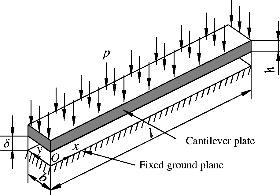
Detail schematic of cantilever plate.

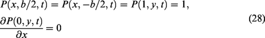
The boundary conditions of the plate are

The free edges y = 0 and y = b

$\frac{{\partial }^{2}w}{\partial y^2}+\mu \frac{{\partial }^{2}w}{\partial x^2}=0$

(2)

$\frac{{\partial }^{3}w}{\partial x^3}+(2-\mu )\frac{{\partial }^{3}w}{\partial x^2\partial y}=0$

(3)

The clamped edge at x = 0

$w(x,y,t)=0,\frac{\partial w}{\partial x}=0$

(4)

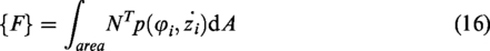
The pressure is governed generally by the nonlinear Reynolds equation²⁴

$\frac{\partial }{\partial x}\left({\delta }^3\overline{p}\frac{\partial \overline{p}}{\partial x}\right)+\frac{\partial }{\partial y}\left({\delta }^3\overline{p}\frac{\partial \overline{p}}{\partial y}\right)=12{\eta }_{eff}\left(\delta \frac{\partial \overline{p}}{\partial t}+\overline{p}\frac{\partial \delta }{\partial t}\right)$

(5)

where $\delta$ is the variable distance between the two plates, $\overline{p}$ is the absolute pressure, and η_eff is the effective dynamic viscosity of air in the gap which accounts for the rarefaction effect through the Knudsen number ⁴²

$K_n=\frac{\lambda }{h_0}=\frac{0.0064\hspace{0.17em}\text{N}/\mathrm{m}}{p_a{h}_0}$

(6)

Here, we use Veijola’s model for estimating the effective viscosity, which is given by

${\eta }_{eff}=\frac{\eta }{1+{9.638}_K{n}^{1.159}}$

(7)

where η is the dynamic viscosity of air under the standard temperature and pressure condition.

The linearized Reynolds equation can be obtained for the isothermal and the inertialess flow under the assumptions of small displacement and the small pressure variation p.

$\delta (x,y,t)={\delta }_0+w(x,y,t),\overline{p}(x,y,t)=p_a+p(x,y,t)$

(8)

where p_a is the ambient pressure, δ₀ is the nominal air gap thickness, δ is the variable air gap thickness. Substituting equation (8) into equation (5) and linearizing the outcome, we obtain

$\frac{{\delta }_0^3}{12{\eta }_{eff}}\left(\frac{{\partial }^{\text{2}}p}{\partial x^2}+\frac{{\partial }^{\text{2}}p}{\partial y^2}\right)=\frac{{\delta }_0}{p_a}\frac{\partial p}{\partial t}+\frac{\partial w}{\partial t}$

(9)

To obtain the pressure distribution corresponding to different modes of vibration, equations (1) and (2) can be solved simultaneously with appropriate boundary conditions. For solving Reynolds equation, the pressure variation p is taken to be zero on the open boundaries while the pressure gradient is taken to be zero on the fixed side.

The pressure boundary conditions for the case in Figure 1 are zero flux at the clamped edges of the plate and trivial pressure at the open edges, that is

$p(x,0,t)=p(x,b,t)=0,\frac{\partial p(0,y,t)}{\partial x}=0$

Modal analysis

To be able to express the governing equation into a discrete form, we need to introduce the concept of a normal coordinate transformation. The continuous displacement w in equation (1) can be expressed as a matrix form

$\left[\mathbf{M}\right]\left\{\ddot{\mathit{w}}\right\}+\left[\mathbf{K}\right]\left\{\mathit{w}\right\}=\left\{\mathit{F}\right\}$

(10)

where [M] is the structural mass matrix, [K] is the structural stiffness matrix, and { F } is the nodal load vector. If the displacement $w(x,y,t)$ is written in terms of n eigenvectors ${\varphi }_i(x,y)$ and a time-dependent modal coordinate $z_i(t)$ as

$w(x,y,t)={\displaystyle \sum _{i=1}^n{\varphi }_i(x,y)z_i(t)}$

(11)

Substituting equation (11) into equation (10), the eigenvectors and the resonant frequencies can be calculated from the dynamic equilibrium equation

$\left[\mathbf{K}\right]\left\{{\varphi }_i\right\}={\omega }_i^2\left[\mathbf{M}\right]\left\{{\varphi }_i\right\}$

(12)

Based on the orthogonal properties of eigenvectors, we obtain the following expression for the resonant frequencies corresponding to different mode shapes

${\left\{{\varphi }_i\right\}}^T\left[\mathbf{K}\right]\left\{{\varphi }_i\right\}={\omega }_i^2{\left\{{\varphi }_i\right\}}^T\left[\mathbf{M}\right]\left\{{\varphi }_i\right\}$

(13)

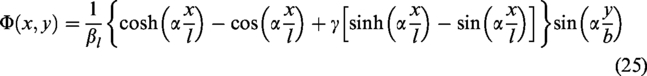
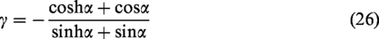
We obtain

${\omega }_i^2=\frac{{\left\{{\varphi }_i\right\}}^T\left[\mathbf{K}\right]\left\{{\varphi }_i\right\}}{{\left\{{\varphi }_i\right\}}^T\left[\mathbf{M}\right]\left\{{\varphi }_i\right\}}=\frac{{\mathit{K}}_i^{*}}{{\mathit{M}}_i^{*}}$

(14)

where

${\left\{{\varphi }_i\right\}}^T\left[\mathbf{K}\right]\left\{{\varphi }_i\right\}={\mathit{K}}_i^{*}\text{\hspace{1em}\hspace{0.17em} and \hspace{1em}\hspace{0.17em}}{\left\{{\varphi }_i\right\}}^T\left[\mathbf{M}\right]\left\{{\varphi }_i\right\}={\mathit{M}}_i^{*}$

(15)

are the modal stiffness and mass of the structure corresponding to the ith eigenvector ${\varphi }_i$ and the resonant frequency ${\omega }_i$ .

To integrate the element pressure, the nodal force vector is calculated at each frequency as

$\left\{F\right\}={\displaystyle {\int }_{area}{N}^{T}p({\varphi }_i,{\dot{z}}_i)\text{d}A}$

(16)

where N^T is the finite element shape function, z_i is the ith modal coordinate, and ${\varphi }_i$ is the ith eigenvector. The total modal force corresponding to each mode is calculated as

${\left\{{\varphi }_i\right\}}^T\left\{\mathit{F}\right\}={\left\{{\varphi }_i\right\}}^T{\displaystyle {\int }_{area}{N}^{T}p({\varphi }_i,{\dot{z}}_i)\text{d}A}$

(17)

The damping and spring coefficients of the squeeze film are calculated from the real and imaginary parts of the mode forces

${\zeta }_{ij}=\frac{{\left\{{\varphi }_i\right\}}^T{\displaystyle {\int }_{area}{N}^T\mathit{Re}\{p({\varphi }_j,{\dot{z}}_j)\}\text{d}A}}{\dot{z}}$

(18)

$K_{ij}=\frac{{\left\{{\varphi }_i\right\}}^T{\displaystyle {\int }_{area}{N}^{T}Im\{p({\varphi }_j,{\dot{z}}_j)\}\text{d}A}}{z}$

(19)

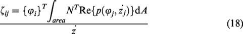
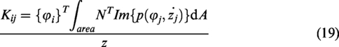
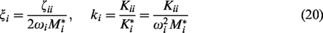
The damping and spring coefficients of each mode due to the squeeze film are the main diagonal entries ζ_ii and K_ii. Off-diagonal terms (i ≠ j) represent the fluidic cross-talk among modes which occurs in the case of asymmetric air gap. The damping ratio ${\xi }_i$ and the spring ratio k_i, which is defined as the ratio of the spring constant due to the squeeze film to the structural stiffness K^*, are calculated from the following expressions

${\xi }_i=\frac{{\zeta }_{ii}}{2{\omega }_i{M}_i^{*}},k_i=\frac{K_{ii}}{K_i^{*}}=\frac{K_{ii}}{{\omega }_i^2{M}_i^{*}}$

(20)

The damping force of the squeeze film and basic damping effects

The gas interacts with the structure surrounding it, while a volume of gas is moved by motion of its confining boundaries. Therefore, it leads to an effect of energy dissipation. This effect demonstrates itself as a damping force on the moving boundary. In general, the behavior of squeeze film is controlled by both viscous and inertial effect within gas. For small geometries in MEMS devices, inertial effect is usually ignored. In such a case, the behavior of fluid is governed by the Reynolds equations. For MEMS devices, the change of temperature is usually negligible due to the small dimensions. Gas density ρ is proportional to its pressure P for the isothermal condition. If δ as well as η_eff is not a function of position, equation (5) can be simplified as

$\frac{\partial }{\partial x}\left(p\frac{\partial p}{\partial x}\right)+\frac{\partial }{\partial y}\left(p\frac{\partial p}{\partial y}\right)=\frac{12{\eta }_{eff}}{{\delta }^3}\left(\frac{\partial p}{\partial t}+\frac{\partial w}{\partial t}\right)$

(21)

The above equation can also be written as

$\frac{{\partial }^2}{\partial x^2}{p}^2+\frac{{\partial }^2}{\partial y^2}{p}^2=\frac{24{\eta }_{eff}}{{\delta }^3}\left(\frac{\partial p}{\partial t}+\frac{\partial w}{\partial t}\right)$

(22)

If the pressure is normalized by ambient pressure p_a, $P(x,y,t)=p(x,y,t)/p_a$ , the nonlinear Reynolds equation for the plate vibration with small amplitude can be written in a nondimensional form

$\frac{{\partial }^2}{\partial x^2}{P}^2+\frac{{\partial }^2}{\partial y^2}{P}^2=2\sigma \left(\frac{\partial P}{\partial t}+\frac{\partial w}{\partial t}\right)$

(23)

where $\sigma ={\alpha }^2{l}^2\omega =\frac{12{\eta }_{eff}{l}^2\omega }{{\delta }_0^2{p}_a}$ is the well-known squeeze number ²² that captures the compressibility effect.

Based on the boundary condition, i.e. clamped x = 0 and free x = l, if the displacement amplitude at the tip is taken as the generalized coordinate Q(t), then at the static equilibrium position, the displacement may be expressed as

$w(x,y,t)=\Phi (x,y)Q(t)$

(24)

where $\Phi (x,y)$ is the exact mode shapes of cantilever plate and is given by^43,44

$\Phi (x,y)=\frac{1}{{\beta }_l}\{\mathit{cosh}\left(\alpha \frac{x}{l}\right)-\text{cos}\left(\alpha \frac{x}{l}\right)+\gamma \left[\mathit{sinh}\left(\alpha \frac{x}{l}\right)-\text{sin}\left(\alpha \frac{x}{l}\right)\right]\}\text{sin}\left(\alpha \frac{y}{b}\right)$

(25)

where $\alpha =1.875104$ for the first mode, 4.694091 for the second mode, and 7.854757 for the third mode, etc. and

$\gamma =-\frac{\mathit{cosh}\alpha +\text{cos}\alpha }{\mathit{sinh}\alpha +\text{sin}\alpha }$

(26)

${\beta }_l=\mathit{cosh}\alpha -\cos \alpha +\gamma (\sinh \alpha -\sin \alpha )$

(27)

Assuming sinusoidal motion $Q(t)=A{e}^{j\omega t}$ ( $j^{\text{2}}=-1$ is imaginary unit), the corresponding nondimensional pressure distribution can be obtained by solving the governing equation with the following boundary conditions

$\begin{array}{l}P(x,b/2,t)=P(x,-b/2,t)=P(1,y,t)=1,\\ \frac{\partial P(0,y,t)}{\partial x}=0\end{array}$

(28)

The normalized pressure distribution under the vibration flexible plate is obtained using Green’s function approach ²³ and is given by

$P(x,y,t)={\displaystyle \sum _{m,n=odd}\frac{16\varpi {(-1)}^{\frac{n+m}{2}-1}}{{\pi }^{2}mn}\frac{-i\omega A{e}^{j\omega t}}{(k_{mn}^2/{\alpha }^2)+j\omega }\text{cos}\left(\frac{m\pi x}{2l}\right)\text{cos}\left(\frac{n\pi y}{b}\right)}$

(29)

in which $k_{mn}={\pi }^2\left(\frac{m^2}{4l^2}+\frac{n^2}{b^2}\right)$ , ${\alpha }^2=\frac{12{\eta }_{eff}}{{\delta }_0^2{p}_a}$ is a constant, and m and n are odd integers, and ϖ is given by

$\varpi =\frac{1}{{\beta }_l}\left[\begin{array}{l}-\frac{m\pi }{2{(-1)}^{\frac{m-1}{2}}}\frac{2{\alpha }^3\gamma }{\left({\alpha }^4-m^4{\pi }^4/16\right)}+\frac{m^2{\pi }^2(\gamma \text{sin}\alpha +\text{cos}\alpha )}{4({\alpha }^2-m^2{\pi }^2/4)}\\ +\frac{m^2{\pi }^2(\gamma \mathit{sinh}\alpha +\mathit{cosh}\alpha )}{4({\alpha }^2+m^2{\pi }^2/4)}\end{array}\right]$

(30)

The total generalized reaction force F(t) on the moving plate is calculated by integrating the pressure distribution $p_{a}P(x,y,t)$ over the domain $S=\left\{(x,y)|0\le x\le l,-b/2\le y\le b/2\right\}$ . So the net force after normalizing it with lbp_a is given by

$\frac{F(t)}{lb{p}_a}=F_{total}={\displaystyle \sum _{m,n=odd}\frac{64{\varpi }^{\text{2}}}{{\pi }^4{m}^2{n}^2}\frac{-j\omega A{e}^{j\omega t}}{k_{mn}^2/{\alpha }^2+j\omega }}$

(31)

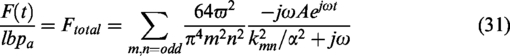
By decomposing the total force F_total into real and imaginary parts, the nondimensional damping force F_d and the spring force F_s are calculated as

$F_d=\frac{64\sigma A}{{\pi }^6}\left({\displaystyle \sum _{m,n=odd}\frac{{\varpi }^{\text{2}}(n^2+m^2{\chi }^2/4)}{m^2{n}^2[{(n^2+m^2{\chi }^2/4)}^2+{\sigma }^2/{\pi }^4]}}\right)\text{cos}\omega t$

(32)

$F_s=\frac{64{\sigma }^{2}A}{{\pi }^8}\left({\displaystyle \sum _{m,n=odd}\frac{{\varpi }^{\text{2}}}{m^2{n}^2[{(n^2+m^2{\chi }^2/4)}^2+{\sigma }^2/{\pi }^4]}}\right)\text{sin}\omega t$

(33)

where $\chi =b/l$ is the aspect ratio of the cantilever plate. Generally, b is the smallest dimension chosen out of length l and width b of the rectangular structure. At the cutoff squeeze number, ${\sigma }_{cutoff}$ , damping and spring forces become equal, if only one term is taken in the summation of equations (32) and (33), then the cutoff squeeze number is approximated by

${\sigma }_{cutoff}={\pi }^2\left(1+{\chi }^2/4\right)$

(34)

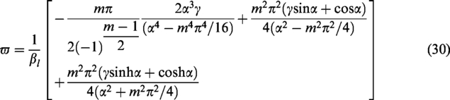
In general, if the plate moves with a low speed, or vibrates in low frequency range, the gas film is not obviously compressed. In this case, the vicious damping force has advantage over and is directly proportional to the speed of plate vibration. On the other side, if plate vibrates with a very high frequency, or moves with a high speed, the gas film is compressed for without enough time to escape. Then, the gas film acts like a spring. The spring force dominates and is directly proportional to the displacement of plate vibration. The corresponding analytical damping constant ζ_a and the spring constant K_a are given by

${\zeta }_a=\frac{p_{a}lb}{\omega {\delta }_0}\frac{64\sigma }{{\pi }^6}{\displaystyle \sum _{m,n=odd}\frac{{\varpi }^{\text{2}}\left(n^2+m^2{\chi }^2/4\right)}{m^2{n}^2\left[{\left(n^2+m^2{\chi }^2/4\right)}^2+{\sigma }^2/{\pi }^4\right]}}$

(35)

$K_a=\frac{p_{a}lb}{{\delta }_0}\frac{64\sigma }{{\pi }^8}{\displaystyle \sum _{m,n=odd}\frac{{\varpi }^{\text{2}}}{m^2{n}^2\left[{\left(n^2+m^2{\chi }^2/4\right)}^2+{\sigma }^2/{\pi }^4\right]}}$

(36)

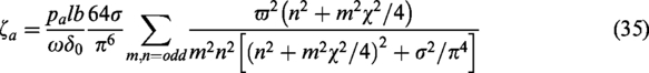
On substituting the value of squeeze number σ in the common term, we obtain the following expression for damping constant ζ_a

${\zeta }_a=\frac{768{\eta }_{eff}l{b}^3}{{\delta }_0^3{\pi }^6}{\displaystyle \sum _{m,n=odd}\frac{{\varpi }^{\text{2}}\left(n^2+m^2{\chi }^2/4\right)}{m^2{n}^2\left[{\left(n^2+m^2{\chi }^2/4\right)}^2+{\sigma }^2/{\pi }^4\right]}}$

(37)

Equation (35) gives the damping constant due to the squeeze film in a cantilever structure in bending modes of vibration. Here, we point out that the effect of different modes comes through ϖ. In the ith resonant mode of plate, the effective mass of the plate oscillating is given by

$m_{eff}=\rho lbh{\displaystyle {\int }_0^l{\phi }^2(x)\mathrm{d}x}$

(38)

Then the damping ratio ξ_a is defined as

${\xi }_a=\frac{{\zeta }_a}{2m_{eff}{\omega }_n}$

(39)

where ${\omega }_n$ is the resonant angular frequency. After substituting the expression of ζ_a in ξ_a, we obtain the following expression of ξ_a

${\xi }_a=\frac{384{\eta }_{eff}{b}^2}{{\Phi }_{1}h\rho {\omega }_n{\delta }_0^3{\pi }^6}{\displaystyle \sum _{m,n=odd}\frac{{\varpi }^{\text{2}}\left(n^2+m^2{\chi }^2/4\right)}{m^2{n}^2\left[{\left(n^2+m^2{\chi }^2/4\right)}^2+{\sigma }^2/{\pi }^4\right]}}$

(40)

which is obtained by substituting ${\Phi }_1={\displaystyle {\int }_0^1{\phi }^2(x)\mathrm{d}x}$ (0.25 for the first mode, 0.249 for the second mode, 0.243 for the third mode, etc.) and ${\omega }_n=\frac{h{\alpha }_b^2}{2l^2}\sqrt{\frac{E}{2\rho }}$ , which is the undamped resonant angular frequency corresponding to the ith mode of the plate with Young’s modulus E and density ρ. The value of ${\alpha }_b=1.875,4.694,7.855$ for the first, second, and third out-of-plane vibration modes of the cantilever plate.

Electrostatic actuation

Static electronic analysis

Electrostatic actuation is the most common method used in MEMS devices because of its excellent scaling properties and ease of integration with COMS electronics. The cantilever beam suspended on top of a polysilicon ground plane can be modeled as a parallel plate capacitor as shown in Figure 2, ignoring fringing effects since the area of the dimensions of the capacitor is much bigger than the gap between the beam and ground plane. ⁴⁵

Figure 2.

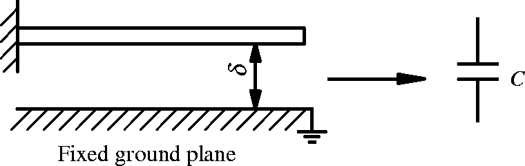
A conducting cantilever plate suspended on top of the ground plane is electrically equivalent to a capacitor C.

For voltage-controlled actuation, the basic parameter is the charge generated by a voltage source as shown in Figure 3. If one plate is moveable and one is fixed, as we have for the case of the cantilever beam, then there are two ways to change the energy. The first one is by changing the charge on the plates, which is accomplished by changing the voltage between the plates. The second way is achieved mechanically by changing the gap between the plates.

Figure 3.

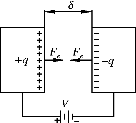
Electrostatic force F_e is from the opposite charges +q and –q built on the plates by the voltage source V.

Quantitatively, the change in energy dW can be expressed as

$dW(q,\delta )=Vdq+F_{e}d\delta$

(41)

where q is the charge on reach surface (beam and ground plane), and δ is the gap between the beam and the ground plane. To obtain the force as a function of the voltage, we need to introduce an abstract term of coenergy W^* defined as

$W^{*}(V,\delta )=qV-W(q,\delta )$

(42)

where $W(q,\delta )$ is the energy expressed in equation (41). Differentially, this becomes

$d{W}^{*}(V,\delta )=(qdV+Vdq)-dW(q,\delta )$

(43)

Substituting equation (41) into equation (43), we have

$d{W}^{*}(V,\delta )=qdV-F_{e}d\delta$

(44)

From this expression, we obtain the equations for q and F_e as a function of coenergy

$q=\frac{\partial W^{*}(V,\delta )}{\partial V}|{\delta }_{=\text{constant}}$

(45)

and

$F_e=-\frac{\partial W^{*}(V,\delta )}{\partial \delta }{|}_{V=\text{constant}}$

(46)

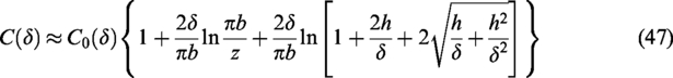
For the structure shown in Figure 2 with a very small distance between the plates (δ ≪ b/2), the capacitance can be approximated by ⁴⁶

$C(\delta )\hspace{0.17em}\approx \hspace{0.17em}{C}_0(\delta )\left\{1+\frac{2\delta }{\pi b}\mathit{ln}\frac{\pi b}{z}+\frac{2\delta }{\pi b}\mathit{ln}\left[1+\frac{2h}{\delta }+2\sqrt{\frac{h}{\delta }+\frac{h^2}{{\delta }^2}}\right]\right\}$

(47)

where $C_0(\delta )=\frac{lb\epsilon {\epsilon }_0}{\delta }$ ( $\delta (x,y,t)\hspace{0.17em}\text{=}\hspace{0.17em}{\delta }_0+w(x,y,t)$ ) is the capacitance by a parallel plate approximation. Equation (47) can be written as $C(\delta )=\vartheta C_0(\delta )$ , where ϑ is a correction factor dependent on the dimensions of the structure

$\vartheta =1+\frac{2z}{\pi b}\mathit{ln}\frac{\pi b}{\delta }+\frac{2\delta }{\pi b}\mathit{ln}\left[1+\frac{2h}{\delta }+2\sqrt{\frac{h}{\delta }+\frac{h^2}{{\delta }^2}}\right]$

(48)

The curves in Figure 4 show the dependence of ϑ on the geometries of the structures and the distance between the bars; it is found that, for typical conditions, as a rule, ϑ ranges from 1.20 to 1.80.

Figure 4.

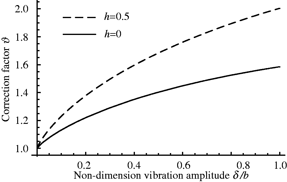
Dependence of ϑ on the dimensions of a structure.

On the other hand, if the distance between the two plates is quite large (δ ≫ b/2), the structure can be approximated as two parallel conductive filaments. The filaments have a circular cross section of radius b/2 and the distance between the two surfaces of the filaments is δ. Based on electrostatic theory, we have

$C(\delta )\hspace{0.17em}\approx \hspace{0.17em}{C}_0\frac{\pi \delta }{b\mathit{ln}(2\delta /b+2)}$

(49)

Therefore, C(δ) is much larger than C₀(δ) for a large distance, but C₀(δ) and C(δ) are both very small so that the differential capacitance between them is not significant.

For a fixed gap capacitor (no mechanical energy variation), while the voltage changes, the coenergy is given by the integral

$W^{*}(V,\delta )={\displaystyle {\int }_0^{V}q\mathrm{d}V}={\displaystyle {\int }_0^{V}CV\mathrm{d}V}={\displaystyle {\int }_0^V\frac{\epsilon A}{\delta }}V\mathrm{d}V$

(50)

where A is the area of the plates and ε is the electrical permittivity. Integrating, we obtain the expression for coenergy W^*

$W^{*}(V,\delta )=\frac{\epsilon A{V}^2}{2\delta }$

(51)

Applying the differential expression of equation (46), we obtain the expression for the electrostatic force F_e

$F_e=\frac{\epsilon A{V}^2}{2{\delta }^2}$

(52)

Note that now the voltage determines the force, which increases z and feeding back to increase the force. This positive feedback results in instability that cause a phenomenon called “pull-in” where the moving plate snaps into the fixed plate. The following section derives the expression for the gap distance where this phenomenon occurs. Of more relevance to this work is pull-in at resonance, which has a different stability criterion from the static pull-in.

To explore the stability of the equilibrium of the plate motion, consider the forces acting on the moving plate. The electrostatic force F_e is pulling the plate down while the elastic force is given by the standard Hooke’s law

$F=kw=k(\delta -{\delta }_0)$

(53)

Consequently, the total force acting on the moving plate is

$F_T=k(\delta -{\delta }_0)-\frac{\epsilon A{V}^2}{2{\delta }^2}$

(54)

The equilibrium condition is $F_T=0$ . To see the effect of small perturbation of the gap $\Delta \delta$ on the force F_T, we can write

$\Delta F_T=\frac{\partial F_T}{\partial \delta }|V_{\Delta }\delta$

(55)

If $\Delta F_T$ is positive for positive $\Delta \delta$ , then that of δ is an unstable equilibrium point because a small increase in $\delta$ creates a force that tends to increase it further (positive feedback). Hence, for stable equilibrium, we need a value of δ that will give a negative $\Delta F_T$ . Evaluating $\Delta F_T$ , we have

$\Delta F_T=\left(\frac{\epsilon A{V}^2}{{\delta }^3}-k\right)$

(56)

For stable equilibrium, this expression has to be negative, giving

$k>\frac{\epsilon A{V}^2}{{\delta }^3}$

(57)

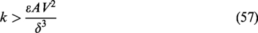
At pull-in, the following equation has to be satisfied

$k=\frac{\epsilon A{V}_p^2}{{\delta }_p^3}\text{\hspace{1em}\hspace{0.17em} and \hspace{1em}\hspace{0.17em}}{F}_T=0$

(58)

where the subscript p indicates value at pull-in. Equating equations (41) and (45), we obtain

$\frac{\epsilon A{V}_p^2}{2{\delta }_p^2({\delta }_0-{\delta }_p)}=\frac{\epsilon A{V}_p^2}{{\delta }_p^3}$

(59)

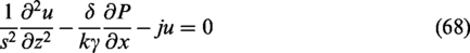
Solving for δ_p, we obtain the point where pull-in occurs

$\delta \frac{=}{23}{\delta }_0$

(60)

This means that for static stability, the plate can move only one-third of gap. Conversely, at resonance, it can be shown that the plate can move up to 0.56 times the gap without having stability problems. The derivation for resonant pull-in is much more involved, and the reader is referred to Seeger and Boser. ⁴⁷ This extra gap allows more room for actuation especially for small-gap electrostatic actuators like those implemented in the standard multiuser MEMS processes.

Electrostatic actuating forces numerical simulation

Figure 5 shows the model geometry according to actual structure. The beam has the following dimension, length 150 µm, width 10 µm, thickness 2 µm. The beam is made of polysilicon with a Young’s modulus, E, of 153 GPa, and a Poisson’s ratio, μ, of 0.23. The polysilicon is assumed to be heavily doped, so that electric field penetration into the structure can be neglected. The beam resides in an air-filled chamber that is electrically insulated. The lower side of the chamber has a grounded electrode. The beam is fixed at one end but is otherwise free to move. An electrostatic force caused by an applied potential difference between the two electrodes bends the beam toward the grounded plane beneath it. To compute the electrostatic force, this example calculates the electric field in the surrounding air. The model considers a layer of air 20 µm thick both above and to the sides of the beam, and the air gap between the bottom of the beam and the grounded layer is initially 2 µm. As the beam bends, the geometry of the air gap changes continuously, resulting in a change in the electric field between the electrodes. The coupled physics is handled automatically by the electromechanics interface.

Figure 5.

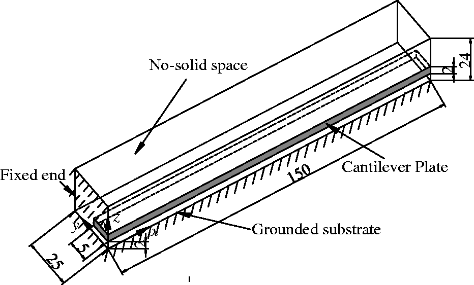
Model geometry. The beam is 150 µm long and 2 µm thick, and it is fixed at x = 0. The model uses symmetry on the zx-plane at y = 0. The lower boundary of the surrounding air domain represents the grounded substrate. The model has 20 µm of free air above and to the sides of the beam, while the gap below the beam is 2.5 µm.

The electrostatic field in the air and in the beam is governed by Poisson’s equation

$-\nabla \cdot \left(\epsilon \nabla V\right)=0$

(61)

where derivatives are taken with respect to the spatial coordinates. The numerical model represents the electric potential and its derivatives on a mesh which is moving with respect to the spatial frame. The necessary transformations are taken care of by the electromechanics interface, which also contains smoothing equations governing the movement of the mesh in the air domain. The cantilever connects to a voltage terminal with a specified bias potential, V_in. The bottom of the chamber is grounded, while all other boundaries are electrically insulated. The terminal boundary condition automatically computes the capacitance of the system.

From the simulated results shown, there is positive feedback between the electrostatic forces and the deformation of the cantilever beam. The forces bend the beam and thereby reduce the gap to the grounded substrate. This action, in turn, increases the force. At a certain voltage the electrostatic forces overcome the stress forces, the system becomes unstable, and the gap collapse. This critical voltage is called the pull-in voltage

$V_{PI}=\sqrt{4{\gamma }_{1}B/\left({\epsilon }_0{l}^4{\gamma }_2^2\left(1+{\gamma }_3{g}_0/w\right)\right)}$

(62)

where V_PI is primarily dependent on the variable B, S, and l. B, S are the bending and stress parameters, as defined in Gupta. ⁴⁸ To the cantilever beam, γ₁ = 0.07, γ₂ = 1.0, and γ₃ = 0.42, respectively. g₀ is the initial gap between the beam and the ground plane; and $B=\tilde{E}{H}^3{g}_0^3$ , $\tilde{E}$ is the plate modulus and equals to E/(1−μ²). μ is the Poisson’s ratio.

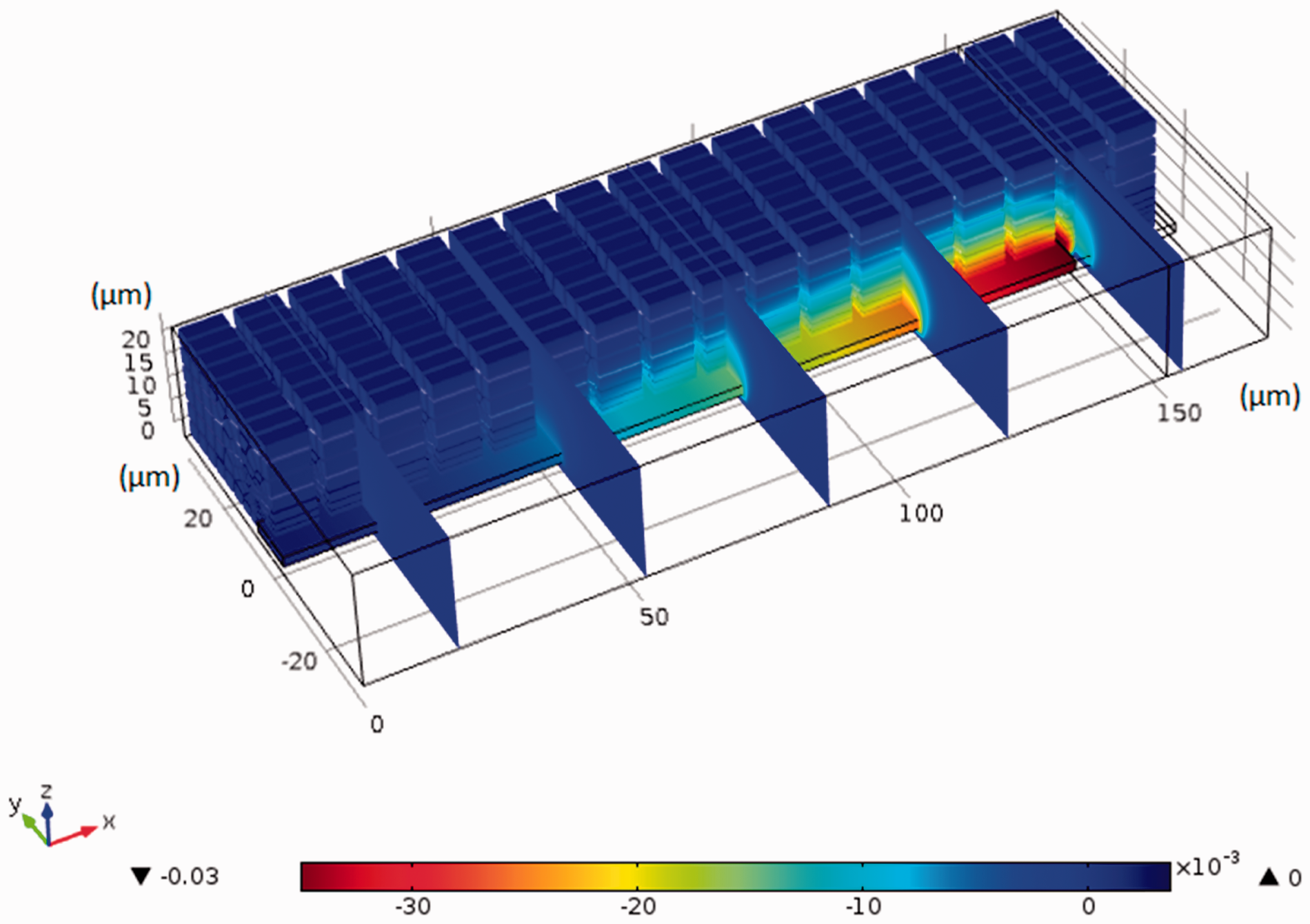
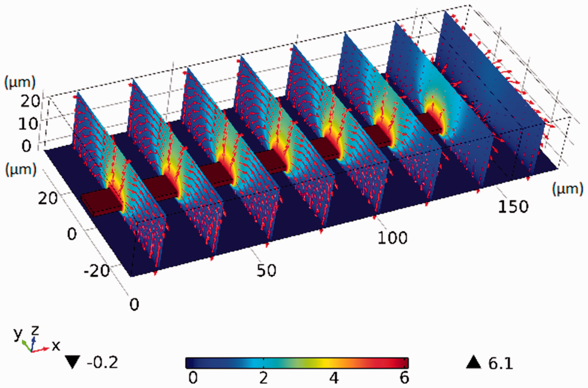
Figure 6 shows the beam displacement and the corresponding displacement of the mesh surrounding it. The tip displacement of beam is maximum. Figure 7 shows the electric potential and electric field that generates these displacements. The color presents the electric potential and the arrows present the electric field. In Figure 8 the shape of the cantilever beam’s deflection is illustrated for each applied voltage, by plotting the z-displacement of the underside of the beam at the symmetry boundary. With the voltage increasing, the static z-displacement gradually becomes bigger. The tip electrostatic force as a function of applied voltage is shown in Figure 9. Below the pull-in voltage, the electrostatic force increases as the driving voltage is rising. In Figure 10, the capacitance between the beam and ground plane is shown for each applied voltage under the critical pull-in voltage. From Figure 10, the higher voltage value causes the bigger capacitance, because the gap becomes smaller under high voltage.

Figure 6.

z-displacement for the beam and the moving mesh as a function of position.

Figure 7.

Electric potential (color) and electric field (arrows) at various cross sections through the beam.

Figure 8.

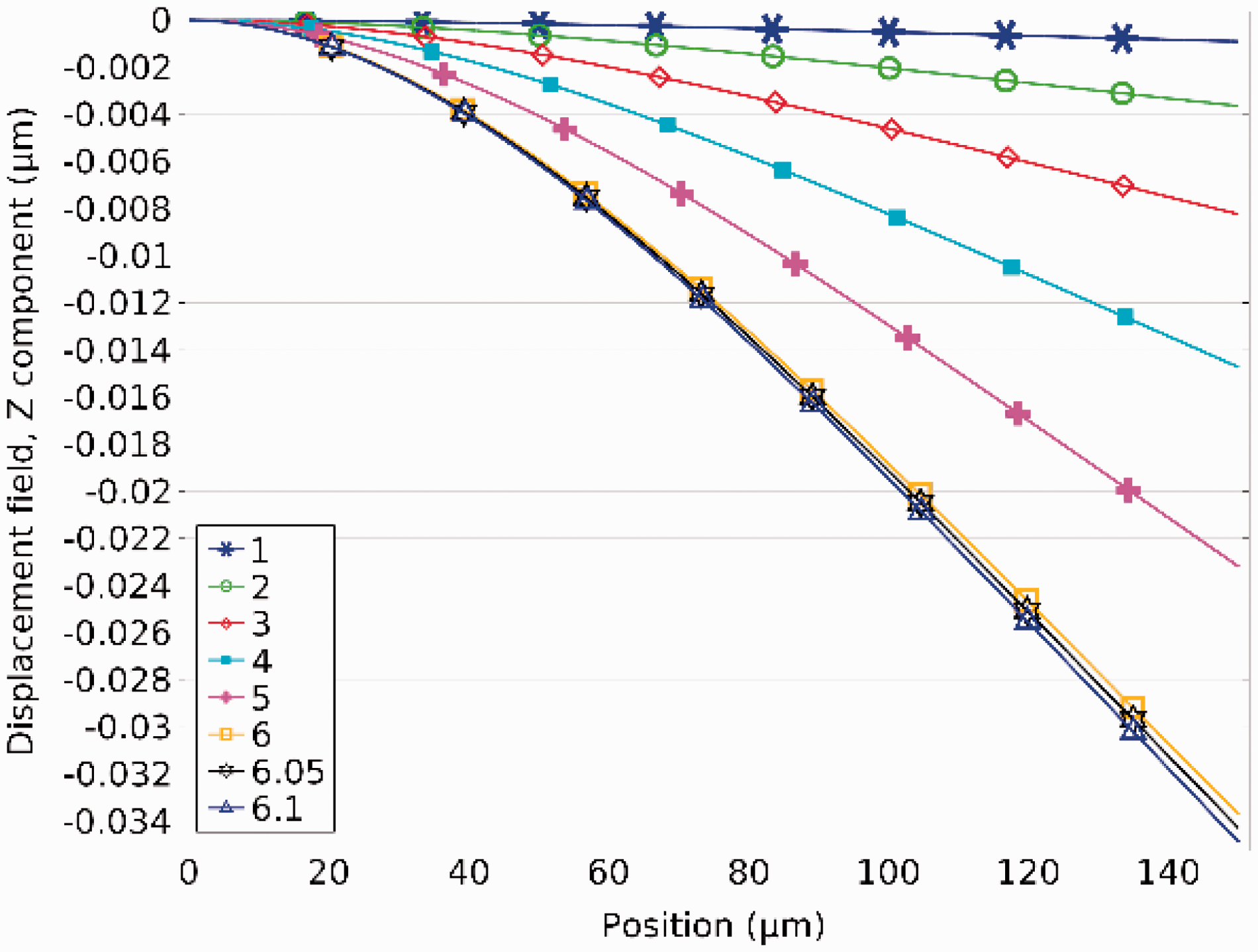
Cantilever beam displacement under different voltage.

Figure 9.

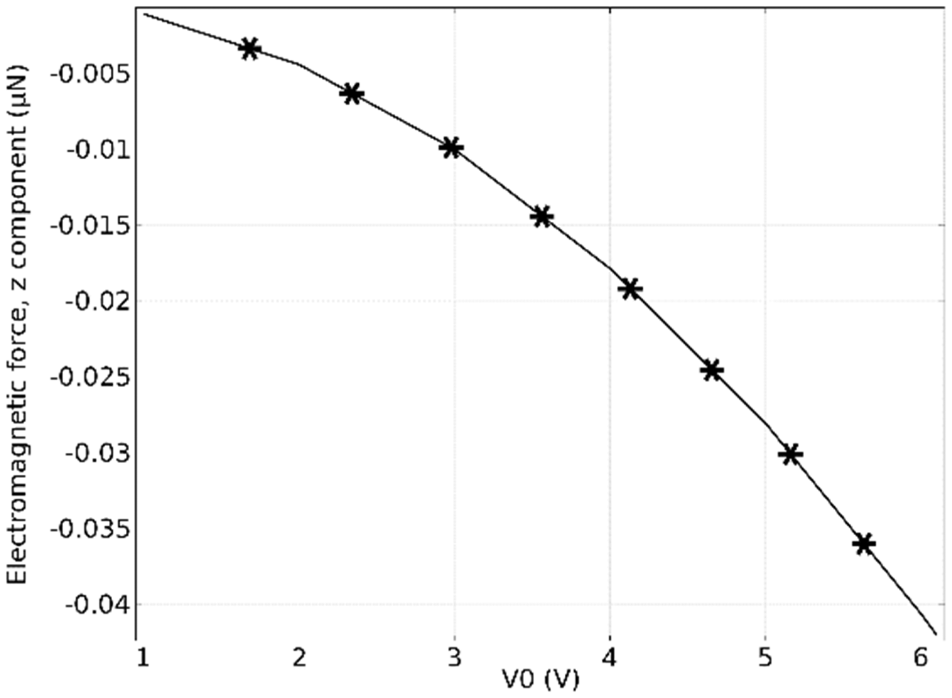
The cantilever tip electrostatic force under the different voltage.

Figure 10.

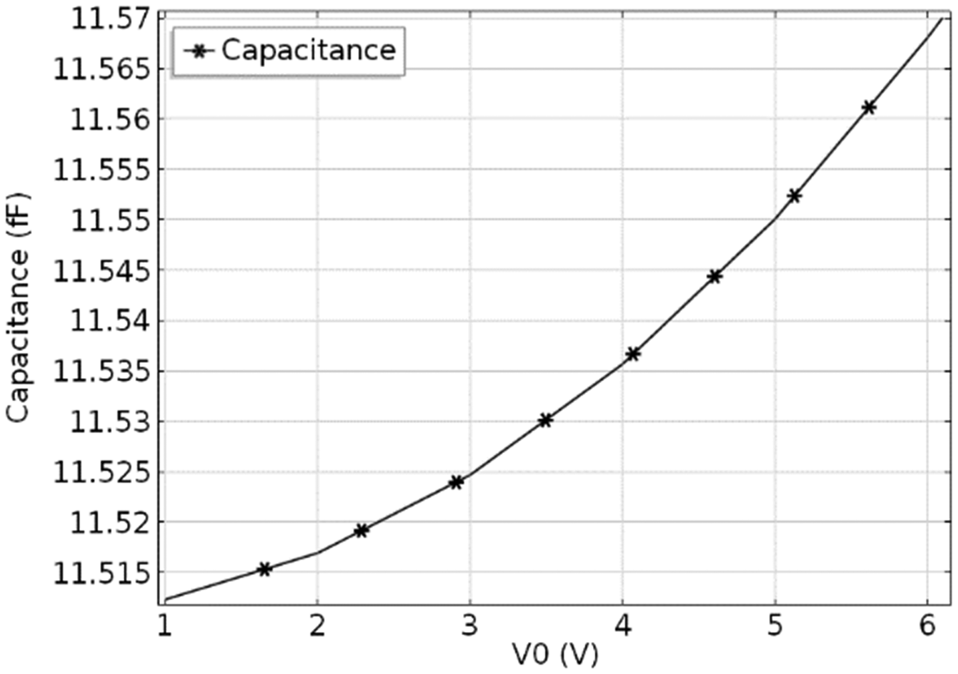
Device capacitance versus applied voltage V₀.

Numerical results of damping

Comparison with other analytical models

There are other simple analytical models that can be used, as appropriate, to predict the modal damping in cantilever resonators due to the squeeze film. The closest among them is the 1D beam model based on exact mode shapes of a 1D beam. ⁴⁶ Since MEMS cantilever resonators seem to have a fairly wide range of length-to-width aspect ratio, depending on their application, it is important to see how the proposed model compares with the existing 1D models. In addition, it is also instructive to compare the proposed model with the simplest known model of rigid parallel plate motion. We now discuss these comparisons before we get into a detailed discussion of comparisons among the numerical, experimental, and the proposed analytical model results.

Under the conditions of incompressible and noninertial flow, the squeeze film damping coefficient with 1D flow assumption across the width of the beam, where the length l of the beam is very large compared to its width b, is given by

${\zeta }_{1D}=\frac{{\eta }_{eff}l{b}^3}{{\delta }_0^3}\frac{m_{eff}}{\rho lbh}=\frac{{\eta }_{eff}l{b}^3}{h^3}{\displaystyle {\int }_0^l{\phi }^2(x)\mathrm{d}x}$

(63)

where $m_{eff}=\rho lbh{\displaystyle {\int }_0^l{\phi }^2(x)\mathrm{d}x}$ . The damping ratio is given by

${\xi }_{1D}=\frac{{\eta }_{eff}{b}^2}{2\rho h{\omega }_n{\delta }_0^3}$

(64)

Subsequently, let us compare the 1D and 2D analytical models, which are given by ξ_1D and ξ_a, with the numerical results shown in Figure 11. We have used cantilever beam of dimensions b = 75 µm, h = 5 µm, δ₀ = 2 µm, χ ∈ [0.1,1], E = 160 GPa, ρ = 2330 kg m³, p_a = 300 Pa, η = 17.2 × 10⁻⁶Pa s, and computed the damping ratios in the first mode of vibration. From Figure 11, ξ_1D have the good results only if χ ≤ 0.1 with an error of < 10%. The numerical and analytical results, which are based on 2D flow, match well with an error of <4.5%. MEMS cantilever resonators with χ > 0.1 are quite common. We see here that for a cantilever resonator even with a small χ = 0.2, the 1D model gives as much as 25% error.

Figure 11.

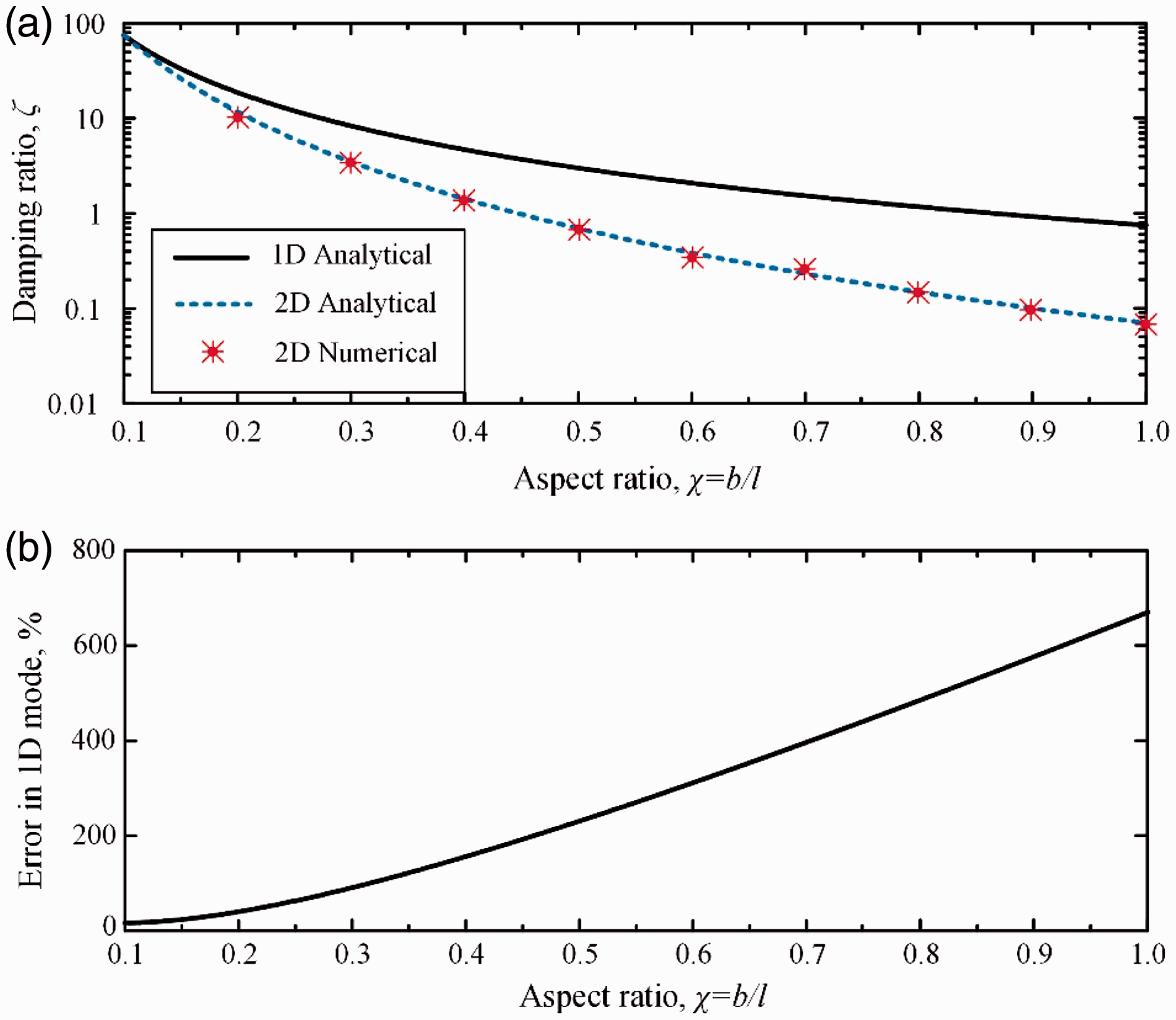
(a) Comparison of 1D and 2D analytical damping ratios with numerical results in the first mode of vibration and (b) error in 1D mode.

Numerical simulation

To study gas flow in the air gap, pressure and velocity of the damper are simulated with multiphysical software. It solves linearized Navier–Stokes equation present as a function of time and frequency. In the study, parameters for air at standard atmosphere conditions are used. The air gap height is δ₀ = 2.5 µm and the length is l = 150 µm. The upper surface oscillates in the z-direction with a constant velocity amplitude of 1 m/s. The action of pressure on the beam bottom is 1000, 300, and 50 Pa.

To demonstrate the damping effect of the gas in the air gap, first, the borders are assumed to be open (zero pressure) and then they are assumed to be closed (zero velocity). Figure 12 shows the pressure distribution on the surface of the proof mass after 1 ms of simulation. The ambient pressure, pA, in three cases is 1000, 300, and 50 Pa, and the acceleration switches on at the beginning of the simulation. The acceleration’s magnitude is half that due to gravity, g. In this figure, the maximum displacement at the tip of the proof mass is roughly 2.4 µm. In Figure 12, from the displacement changes seen, the phase of damping force occurs variation.

Figure 12.

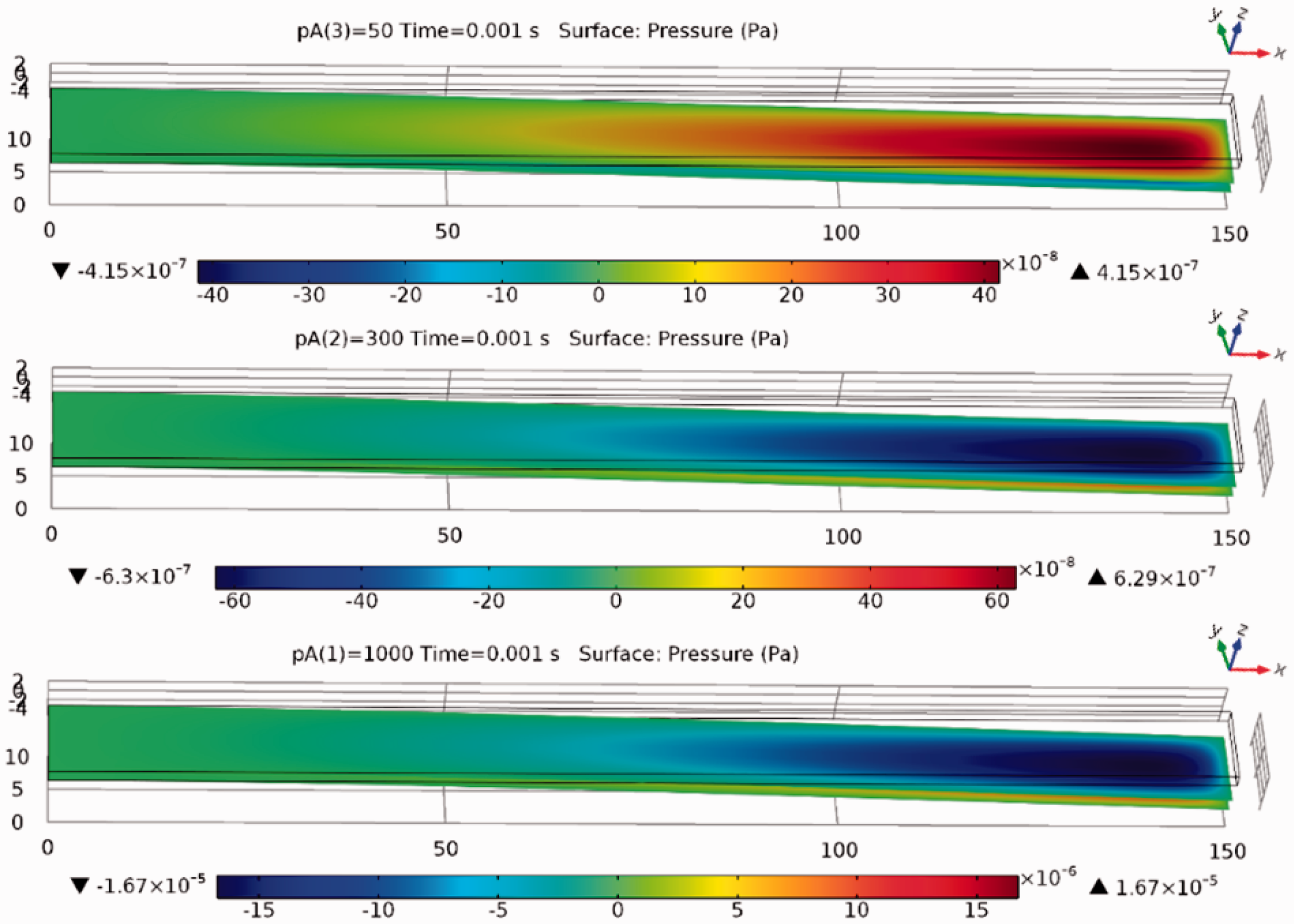
The pressure distribution on the face of the proof mass in the z-direction leads to a deformation.

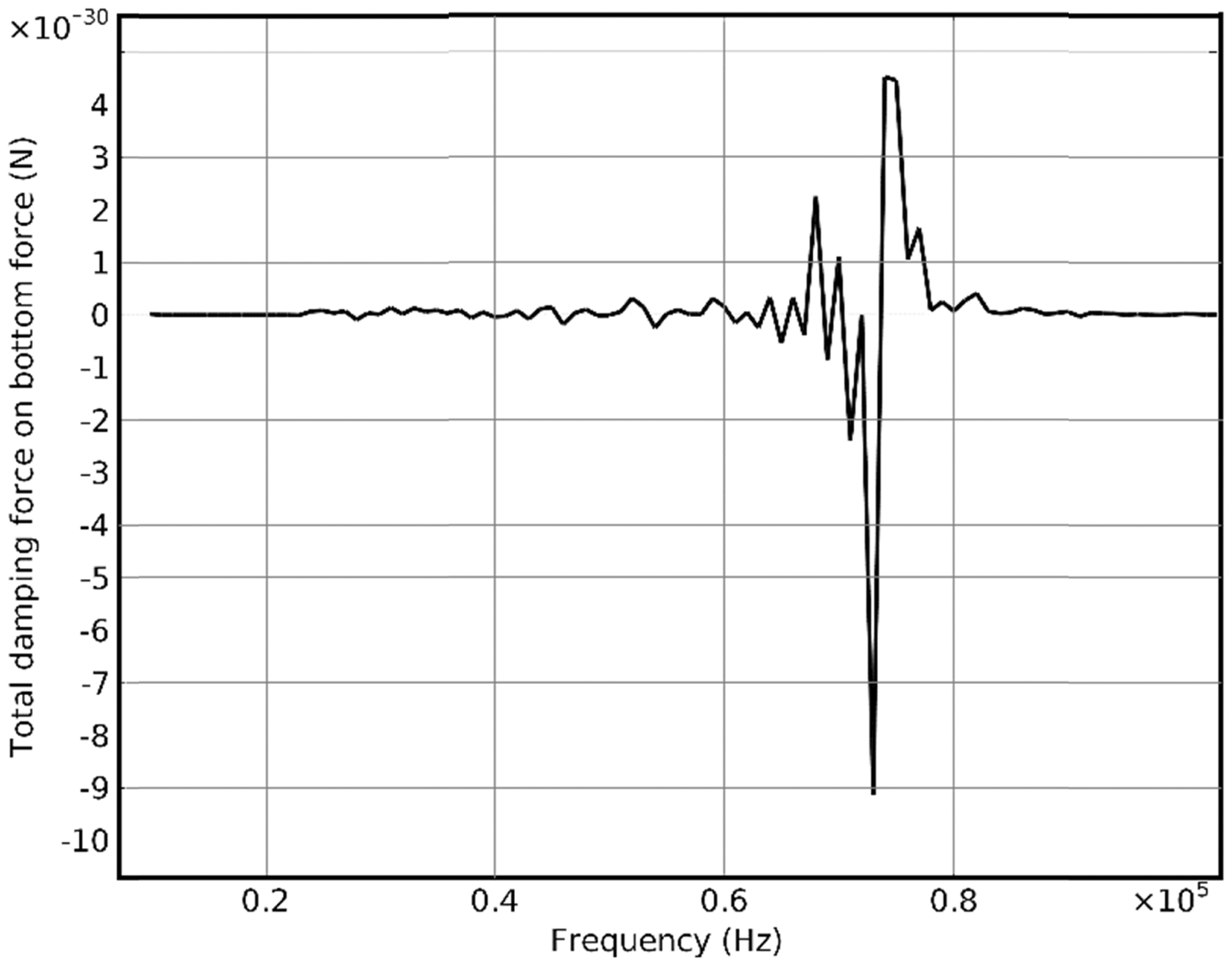
The bottom force of air thin film acting on the surface is shown in Figure 13 at different frequencies. With the frequencies increment, the forces are gradually decreasing which this variation is more apparent under higher ambient pressure. At the low frequency, the direction of bottom force at low ambient pressure is contrary to at high one. In Figure 14, the damping forces of bottom are shown, and the changes of forces occur at near resonant frequency. In other words, the damping effects are stronger at resonant frequency, and the magnitude of damping action in relation to the ambient pressure, at 300 Pa, the damping force being minimum. The amplitude variation of damping force is larger at low ambient pressure of 50 Pa. Thus, this illustrates that the damping force can be strongly influenced by the pressure of gas gap. The amplitude responses are identical above a certain frequency indicating that at high frequencies the flow velocity in the x-direction becomes insignificant. Hence, at high frequencies the gas is trapped in the gap corresponding to the closed border assumption, even for open border conditions.

Figure 13.

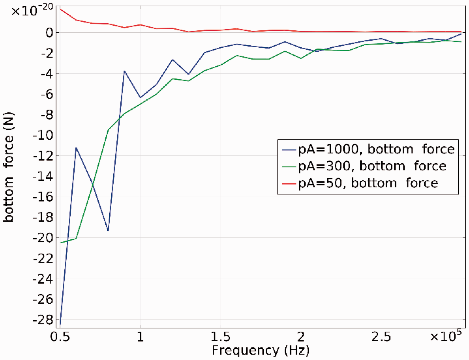
The bottom forces of the proof mass tip at ambient pressures of 1000, 300, and 50 Pa at function of frequencies.

Figure 14.

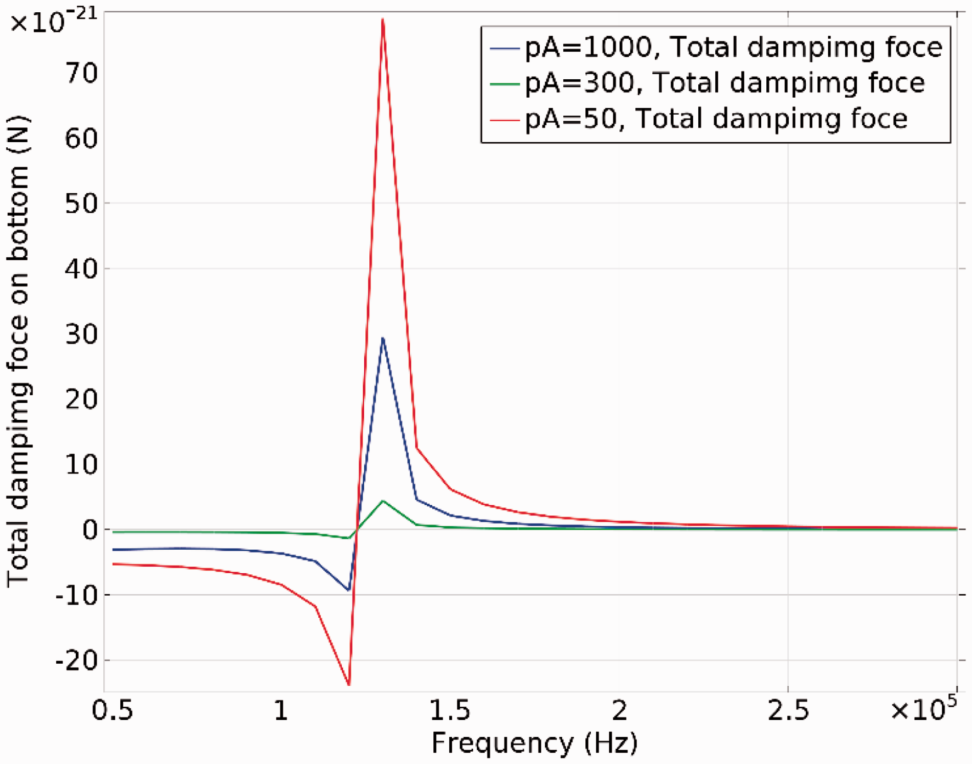
The damping force of bottom surface at ambient pressures of 1000, 300, and 50 Pa as function of frequency.

Figure 15.

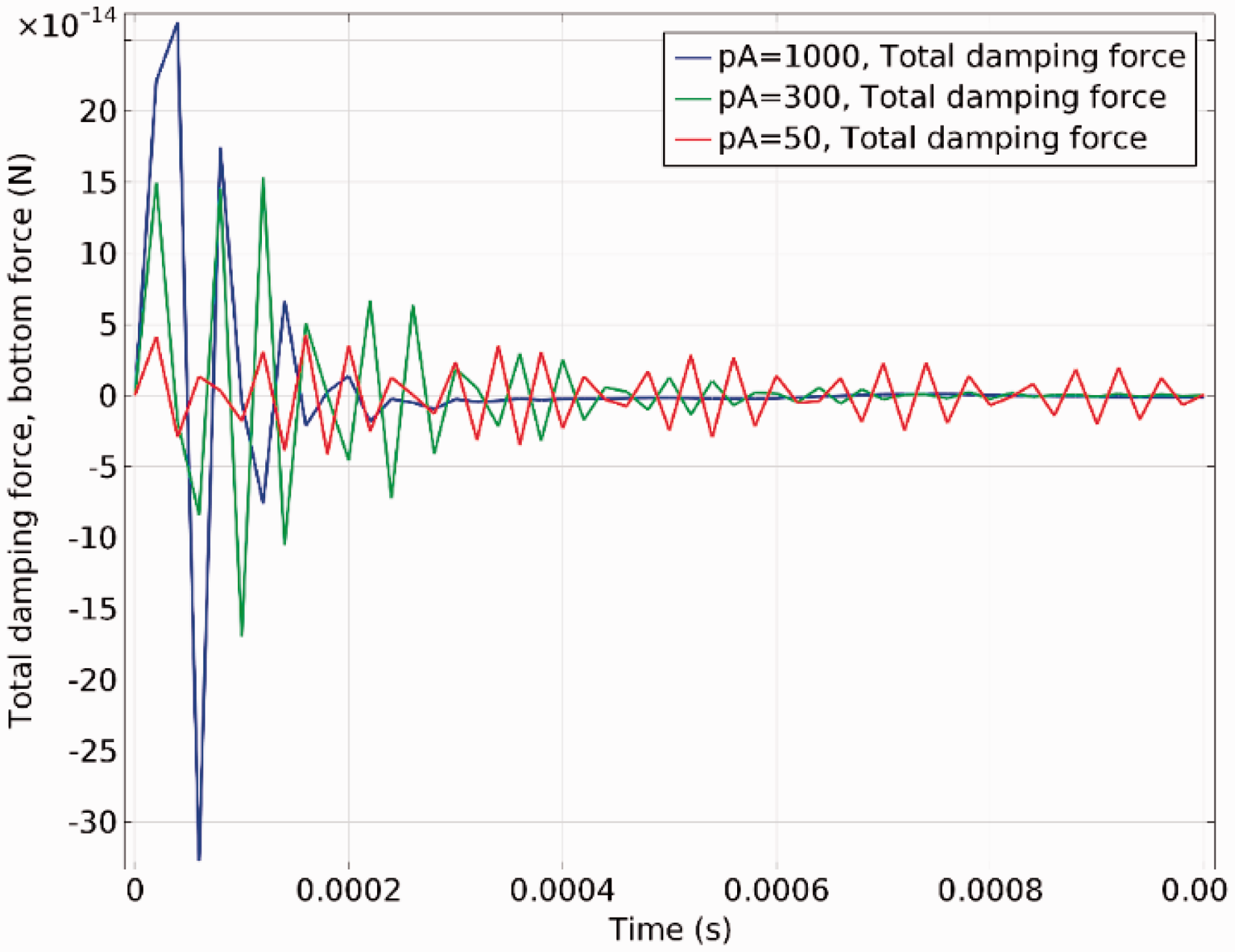
The damping forces of bottom as function of time at the ambient pressures of 1000, 300, and 50 Pa.

The damping forces and tip displacements of beam bottom are shown in Figures 15 to 17. The damping forces gradually drop off over time. The higher ambient pressure can constrain the wave of damping force and produce the larger total forces. The numerical results are shown in Figure 16; it is just that the declining process becomes lengthy. The amplitude responses of tip displacement of beam become bigger at the low ambient pressure as shown in Figure 17. Meanwhile, the nonlinear traits are also presented. Corresponding to Figure 12, large displacement means higher surface perssure.

Figure 16.

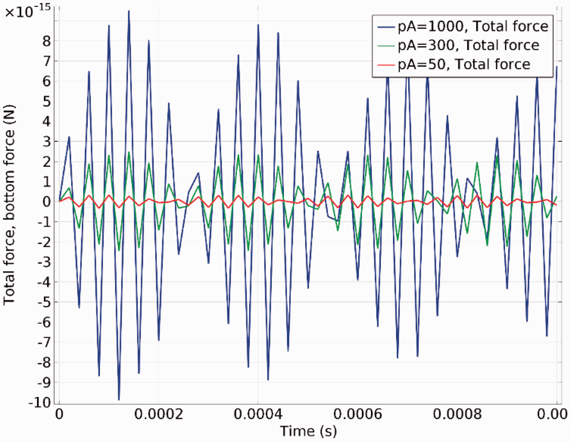
The total force of bottom as function of time at the ambient pressures of 1000, 300, and 50 Pa.

Figure 17.

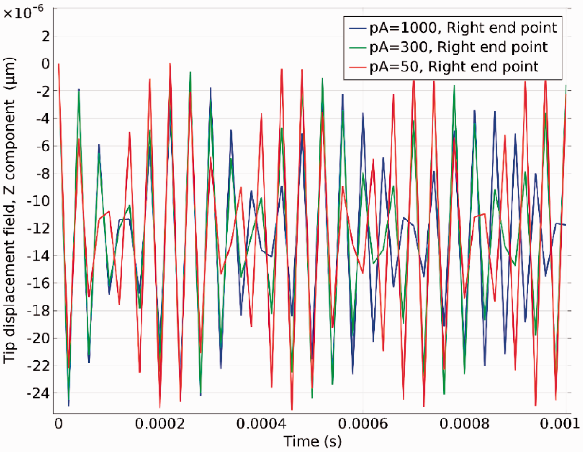
The tip displacement of beam as function of time at the ambient pressures of 1000, 300, and 50 Pa.

Analyzing resonance region of compact model squeeze film damping

The lower frequency (squeeze film damping) region is studied in order to derive the compact model for the mechanical impedance of the damper. Linearized dimensionless form of the Navier–Stokes equations is derived based on Beltman et al. ⁴⁹ The equations are in 2D (y-direction and temperature are not considered and the structure becomes a beam)

$\frac{\text{4}{\delta }_a^2}{\text{3}{s}^2}\frac{{\partial }^{2}u}{\partial x^2}+\frac{\text{1}}{s^2}\frac{{\partial }^{2}u}{\partial z^2}+\frac{{\delta }_a}{3s^2}\frac{{\partial }^{\text{2}}w}{\partial x\partial z}-\frac{{\delta }_a}{k\gamma }\frac{\partial P}{\partial x}-ju\hspace{0.17em}\text{=0}$

(65)

$\frac{{\delta }_a^2}{s^2}\frac{{\partial }^{2}w}{\partial x^2}+\frac{4}{3s^2}\frac{{\partial }^{2}w}{\partial z^2}+\frac{{\delta }_a}{3s^2}\frac{{\partial }^{2}u}{\partial x\partial z}-\frac{1}{k\gamma }\frac{\partial P}{\partial z}-jw=0$

(66)

${\delta }_a\frac{\partial u}{\partial x}+\frac{\partial w}{\partial z}=-jk\rho$

(67)

where, $s=h_0\sqrt{{\rho }_0\omega /\mu }$ shear wave number. u and w are velocity components in the x- and z-directions, respectively. γ is ratio of specific heats. The equations are in normalized form such that velocities u and w are normalized to the speed of sound c₀ and the dimensions x and z are normalized with the characteristic dimensions l and δ, respectively. P and ρ represent small relative variation around P₀ and ρ₀, respectively. The narrowness of the gap is ${\delta }_a=\delta \text{/}l$ .

For deriving the compact model, a reduced set of NS equations is needed. The complete set of 2D equations will be reduced by removing insignificant terms. Since velocity u varies less in the x-direction than in the z-direction, and g is small, term ${\partial }^{2}u/\partial x^2$ can be ignored. Also, due to translational velocity excitation, the term $\partial w/\partial x$ is very small and is ignored here. At low frequencies, k is small and equation (66) reduces simply to $\partial P/\partial z=0$ . At high frequencies, ${\partial }^{2}w/\partial x^2$ is small due to the excitation, and $\partial u/\partial x$ is small in equation due to trapped situation. The reduced equations are

$\frac{1}{s^2}\frac{{\partial }^{2}u}{\partial z^2}-\frac{\delta }{k\gamma }\frac{\partial P}{\partial x}-ju=0$

(68)

$\frac{1}{s^2}\frac{{\partial }^{2}u}{\partial z^2}-jw=0$

(69)

${\delta }_a\frac{\partial u}{\partial x}+\frac{\partial w}{\partial z}=-jk\rho$

(70)

An approximate solution for the above equations is presented as follows. First, the equations are further reduced to have the trapped air situation. This is accomplished assuming flow in the z-direction only, that is u(x)=0, and solving the velocity profile w(z). Next, the narrow gap situation is assumed ignoring equation (66) and a differential equation for the pressure distribution is derived. Finally, the flow profile w(z) is inserted in the differential equation that is solved for perpendicular motion and zero pressure boundary conditions.

Next, the lower frequency (squeeze film damping) region is studied in order to derive the compact model for the mechanical impedance of the damper. This is accomplished by using the equations (68) to (70) for narrow gap problems, that is equation (69) will be ignored in the following analysis.

Equation (68) can be solved when P = P(x) yielding

$u=\frac{j{\delta }_a}{k\gamma }\frac{\partial P}{\partial x}A\left(s,K_n,z\right)$

(71)

where

$A(s,K_n,z)=1-\frac{\mathit{cosh}\left[\sqrt{j}s(z\frac{-}{12})\right]}{\mathit{cosh}(\sqrt{j}s/2)+\sqrt{j}s{K}_n\mathit{sinh}(\sqrt{j}s/2)}$

(72)

The Knudsen number K_n = λ/δ₀ is a measure of gas rarefaction.

The differential equation for the pressure distribution in the x-direction is derived from equation (70) by averaging the velocity u and density ρ across the gap

${\delta }_a{\displaystyle {\int }_0^1\frac{\partial u}{\partial x}}\mathrm{d}z+jk{\displaystyle {\int }_0^1\rho \mathrm{d}z}=-{\frac{\partial w}{\partial z}|}_{z=1}$

(73)

where the density can be represented as $\rho =P{\left[1-\frac{\gamma -1}{\gamma }A(s,K_n,z)\right]}^{-1}$ .

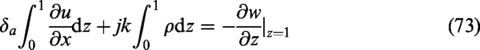
Since the mechanical impedance is specified at z = 1, the term in the right-hand side has not been averaged across the gap. Instead of the average velocity in the z-direction, the velocity excitation at the upper surface (z =1) is used here.

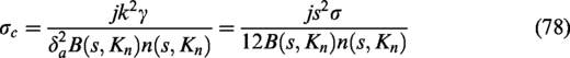
Inserting u and ρ into equation (73) gives a general frequency domain model for 1D air gaps

$\frac{{\delta }_a^{2}B(s,K_n)}{jk\gamma }\frac{{\partial }^{2}P(x)}{\partial x^2}-\frac{jk}{n(s,K_n)}P(x)={\frac{\partial w}{\partial z}|}_{z=1}$

(74)

where

$B(s,K_n)={\displaystyle {\int }_0^{1}A(s,K_n,z)\mathrm{d}z}=\frac{\sqrt{j}s-(2-j{s}^2{K}_n)\mathit{tanh}(\sqrt{j}s/2)}{\sqrt{j}s+\text{i}{s}^2{K}_n\mathit{tanh}(\sqrt{j}s/2)}$

(75)

$n(s,K_n)={\left[1-\frac{\gamma -1}{\gamma }B\left(s,K_n\right)\right]}^{-1}$

(76)

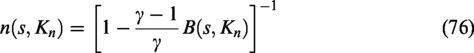
The function n is the result of thermal effects. It is generally complex valued signifying a phase shift between the pressure and density perturbation. Hence, it models the losses due to gas compressibility that are important in the transition regime when conditions change from isothermal to adiabatic. At low frequencies (s ≪ 1), the flow is isothermal leading to n = 1 and at high frequencies (s ≫ 1), B(s, K_s) approaches 1 and n→γ (adiabatic conditions).

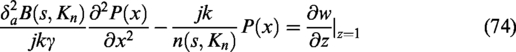
Equation (74) is solved with trivial pressure boundary conditions P(±l/2)=0. The solution is searched in the form P(x) = bcosh(cx) + d, yielding

$P(x)=\frac{n(s,K_n)}{jk}\left[\frac{\mathit{cosh}(\sqrt{j{\sigma }_c}x)}{\mathit{cosh}\left(\sqrt{j{\sigma }_c}/2\right)}\right]{\frac{\partial w}{\partial z}|}_{z=1}$

(77)

where σ_c is the complex squeeze number

${\sigma }_c=\frac{j{k}^2\gamma }{{\delta }_a^{2}B(s,K_n)n(s,K_n)}=\frac{j{s}^2\sigma }{12B(s,K_n)n(s,K_n)}$

(78)

It specifies the ratio between the spring force due to the gas compressibility and the force due to the viscous flow.

The resulting force acting on the surface is

$F={\displaystyle {\int }_{-1/2}^{1/2}{\displaystyle {\int }_{-1/2}^{1/2}P(x)\mathrm{d}x\mathrm{d}y}}=\frac{n(s,K_T)}{jk}\left[\frac{2}{\sqrt{\text{i}{\sigma }_c}}\mathit{tanh}\left(\sqrt{j{\sigma }_c}/2\right)-1\right]{\frac{\partial w}{\partial z}|}_{z=1}$

(79)

where the velocity excitation is calculated when z = 1.The velocity functions ∂w/∂z can been solved from equations (65) to (67).

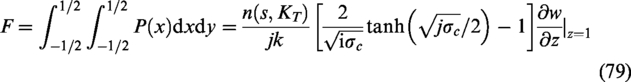
The un-normalized force becomes

$\tilde{F}=-\frac{lDn(\phi s,K_T)P_0}{j\omega {\delta }_0}\left[\frac{2}{\sqrt{j{\sigma }_c}}\mathit{tanh}\left(\sqrt{j{\sigma }_c}/2\right)-1\right]{\frac{\partial w}{\partial z}|}_{z={\delta }_0}$

(80)

The above equation is the complete model to calculate the force as a function of frequency for a velocity excitation. The damping force is the real part of $\tilde{F}$ .

In the following, the numerical results of the compact model are compared to numerical FEM simulations which can be considered as exact results. The model is $l=15$ µm, $h=1.2$ µm, and ${\delta }_0=1$ µm. Then, the importance of the included features in the compact model is studied by comparing the response of published models in a wide low frequency band. In the following figures, the damping force of compact model on the bottom face is denoted in Figure 18. Gas parameters for air with the same dimensions as in previous discussions were to be used in the simulations.

Figure 18.

The damping force of compact model at low frequency for a velocity excitation.

The pressure values are calculated for each mode. Once the pressures for each element are known, they are integrated to compute the force vector for each frequency. The scalar products of all vectors are then computed―the scalar products represented the modal forces and they state how much of the pressure distribution acts on each mode. The pressure can be used to determine two matrices: the modal damping coefficient matrix C_ii and the modal squeeze stiffness matrix K_ij. The subscript i represents the deflection mode (source mode) while subscript j represents the mode experiencing the pressure (target mode). The diagonal terms of the matrices represent the coefficients for each mode while the off-diagonal terms represent the cross-talk between modes. The damping ratio ζ_i for mode i can be obtained from the matrix coefficient C_ii as ζ_i = C_ii/2ω_im_i, where ω_i is resonant frequency of mode i and m_i is the modal mass.

The pressure values are calculated for each mode. Once the pressures for each element are known, they are integrated to compute the force vector for each frequency. The scalar products of all vectors are then computed―the scalar products represented the modal forces and they state how much of the pressure distribution acts on each mode. The pressure can be used to determine two matrices: the modal damping coefficient matrix C_ii and the modal squeeze stiffness matrix K_ij. The subscript i represents the deflection mode (source mode) while subscript j represents the mode experiencing the pressure (target mode). The diagonal terms of the matrices represent the coefficients for each mode while the off-diagonal terms represent the cross-talk between modes. The damping ratio ζ_i for mode i can be obtained from the matrix coefficient C_ii as ζ_i=C_ii/2ω_im_i, where ω_i is resonant frequency of mode i and m_i is the modal mass.

The analysis was performed for the cantilever beam with the same dimensions as in previous discussions and the results were compared to the approximation based on the simplified Reynolds equation from the aforementioned content. A variation of several parameters was performed and the comparison between the two results plotted. Figure 19 shows the damping coefficient as a function of resonant frequency of the beam. There is a good agreement with the analytical data and FEM results. It can be seen that the lower the resonant frequency of the beam was small damping coefficient. The damping coefficient reaches the peak near the first mode frequency, but the damping rapidly drops to a low level by increasing the frequency. From analytical results shown, the resonant frequency can be varied by changing the thickness of the beam. However, this has no effect on the squeezed film since the surface of the beam interacting with the fluid remains the same.

Figure 19.

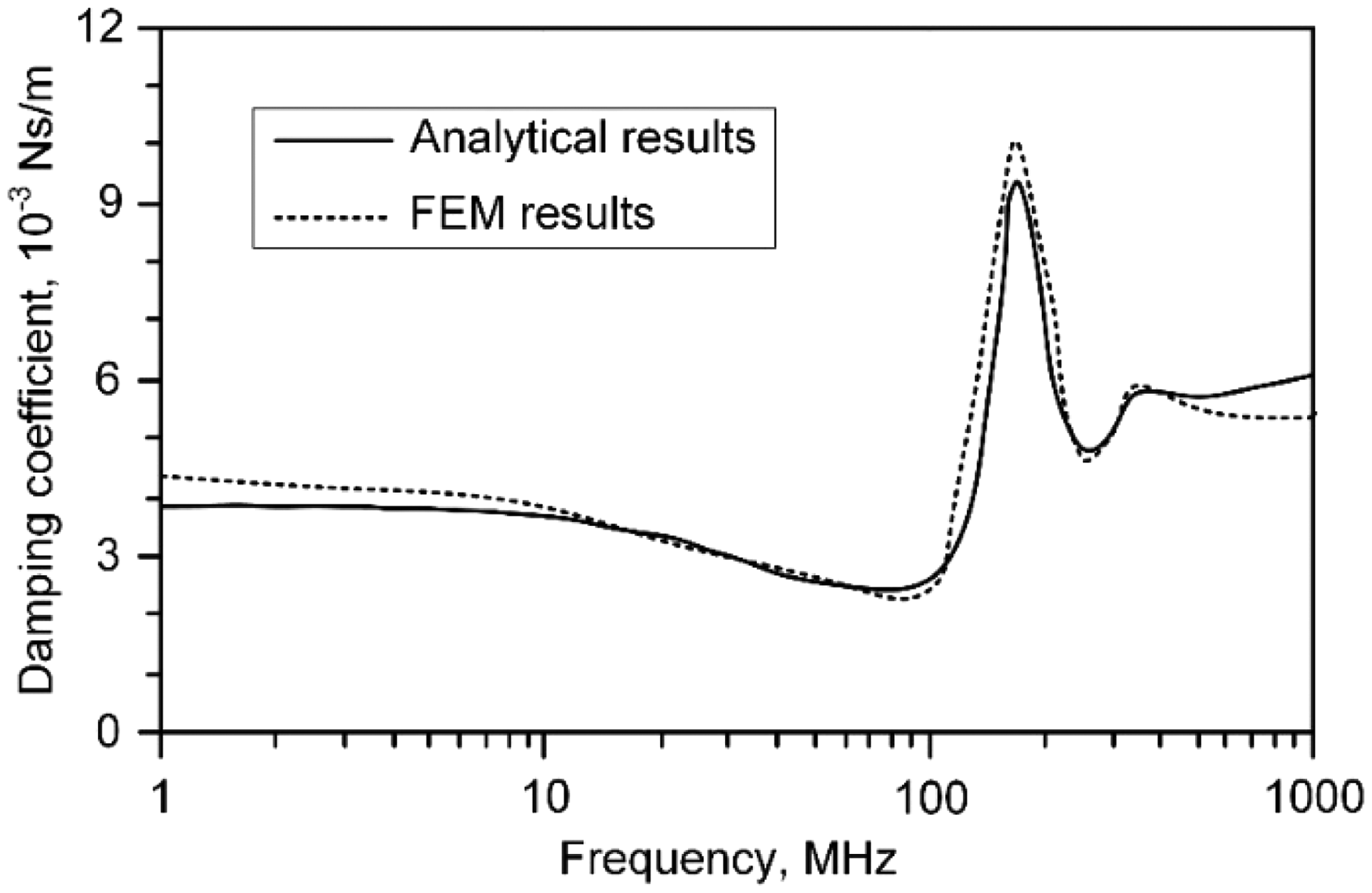
The damping coefficient as calculated by an analytical approximation based on simplified Reynolds equation compared to the value by FEM for the first model. FEM: finite element method.

Conclusion

With these models, analysis and simulation of a MEMS-based cantilever plate acting as a precise mass sensor in viscous environments were performed. The analytical framework for the modeling of the cantilever plate sensor is provided. Most of the physical phenomena are governed by PDEs and their associated boundary and initial conditions. Even though, for most cases, the PDEs have no closed-form solutions, it is useful to understand their derivation and approximate analytical solutions as these provide insight on the phenomena. For more accurate results, numerical methods are applied for analyzing electrostatic actuation and damping of squeeze film. Electrostatic actuation was proposed for driving the cantilever to overcome the thermal noise and coupled domain electrostatic-structural simulations were performed to calculate the displacement of the beam as a function of the voltage applied. By using modal discrete technique, damping force was calculated for the modes of vibration and it was found that the high order modes of vibration are less affected. The Reynolds equation has been extended to be applicable to rapidly oscillating surfaces and rarefied gas conditions in addition to modeling damping at low frequencies. It was shown that the compact model is in good agreement with numerical FEM simulation results.