Sage Journals: Discover world-class research

Abstract

The research performed in this paper is carried out to calculate the sound pressure level of the marine propeller by Reynolds-Averaged Navier–Stokes solver in low frequencies band. Noise is generated by the induced trailing vortex wake and induced pressure pulses. The two-step Fflowcs Williams and Hawkings equations are used to calculate hydrodynamic pressure and its performance as well as sound pressure level at various points around the propeller. The directivity patterns of this propeller and accurate explanation of component propeller noise are discussed. Comparison of the numerical results shows good agreement with the experimental data.

Keywords

Marine propeller sound pressure level hydrodynamic performance

Introduction

Various factors, including environmental and structural factors play an important role in the generation of underwater noise. Ship’s propeller creates noise from its working behind the ship to make the thrust for overcoming the resistance at designed speed. Noise generated by the propellers in terms of intensity and spectral is a strategic issue for warships and military designers over the years.¹ The generated sound can be heard for hundreds of meters below the surface and may be detected by the sonar. In design process of marine propeller, to the extent possible, the amount of the noise level should be minimal.² Generally, there are two main sources of noise: one is due to mechanical elements like engine and second one is by hydrodynamic source, i.e. by the propeller.³ Research is needed on the noise sources in order to reduce the noise and increase performance quality by making minimal changes in the vessels’ elements.⁴

Propeller noise usually includes a series of periodic parts, or tones, at blade rate and its multiples. These periodic unsteady forces impose discrete tonal noise at the blade-passing frequency (BPF)⁵ together with a broadband noise spectrum caused by turbulence interaction with blade and vortex shedding at the trailing edge and the tips. A small-scale part of turbulent eddies in the wake causes unsteady blade forces. Besides, the boundary layer separation and blades vortex shedding also causes fluctuating forces. Shedding vortex will happen at the area of trailing edge and tip of rotating blades. Induced pressure pulses by the propeller may consider one of the important sources in the sound pressure level (SPL). Moreover, whereas the propeller operates in the heavy-load condition, the boundary layer around the blade may separate at the stagnation point in the suction side. The flow separation and vortex shedding are completely unsteady event, which will impose oscillating pressure on the propeller. So, the underwater propeller will produce noise, even in uniform inflow.⁶

Conventional procedures to study the propeller unsteady force are the lifting surface and the panel methods. Kerwin and Lee⁷ applied the unsteady vortex lattice technique to formulate the unsteady propeller. Hoshino⁸ employed the panel method to simulate unsteady flow on the propeller. These methods do not account for viscous effects, such as the boundary layer and separation flow and usually repair results with empirical treatments. To conquer the deficiency of potential methods, Reynolds-Averaged Navier–Stokes (RANS) model has been successfully employed for marine propellers. Funeno⁹ studied unsteady flow around a high-skewed propeller in nonuniform inflow. Hu et al.¹⁰ applied RANS model to simulate the test case, DTMB 4119, propeller working on nonuniform inflow conditions. Li and Yang¹¹ investigated the numerical prediction of flow around a propeller. Numerical simulation of tonal and broadband hydrodynamic noises of noncavitating underwater propeller was carried out by Kheradmand et al.¹² Seol et al.¹³ presented a numerical study on the noncavitating and blade sheet cavitation noises of the underwater propeller. The noise is predicted using time-domain acoustic analogy while the flow field is analyzed with potential-based panel method. Park et al.¹⁴ numerically analyzed the tip vortex cavitation behavior and sound generation. In their work, they used hybrid method which integrates RANS solver and dissipation vortex model for flow field. Seol et al.¹⁵ used boundary element method to predict the noncavitation noise of a ducted propeller in various different operating conditions and configurations. Wang et al.¹⁶ have done an extensive and precise study in 2006 on the effects of the propeller’s trailing edge on the radiated noise. In this study, using numerical simulations, optimization of the trailing edge geometry was investigated. Jang et al.¹⁷ analyzed BPF noise of a propeller comprising of the thickness and loading noises on noncavitating marine propeller.

The objective of the current study is to conduct a numerical simulation of the acoustic pressure generated by a marine propeller under uniform flows in low frequencies band. The far-field radiation is predicted by integral formula Fflowcs Williams and Hawkings (FW-H) equation, with the solution of the RANS solver. The hydroacoustic performances of propeller are compared with experimental study. All flow and acoustic simulations and postprocessing calculations of the data are performed with the commercial software ANSYS 14.0.

Wide range of frequencies of the propeller noise

A wide range of frequencies (low and high frequency) exist in propeller noise as described below. Frequency domain shows the range of underwater noise frequencies in Figure 1.

Figure 1.

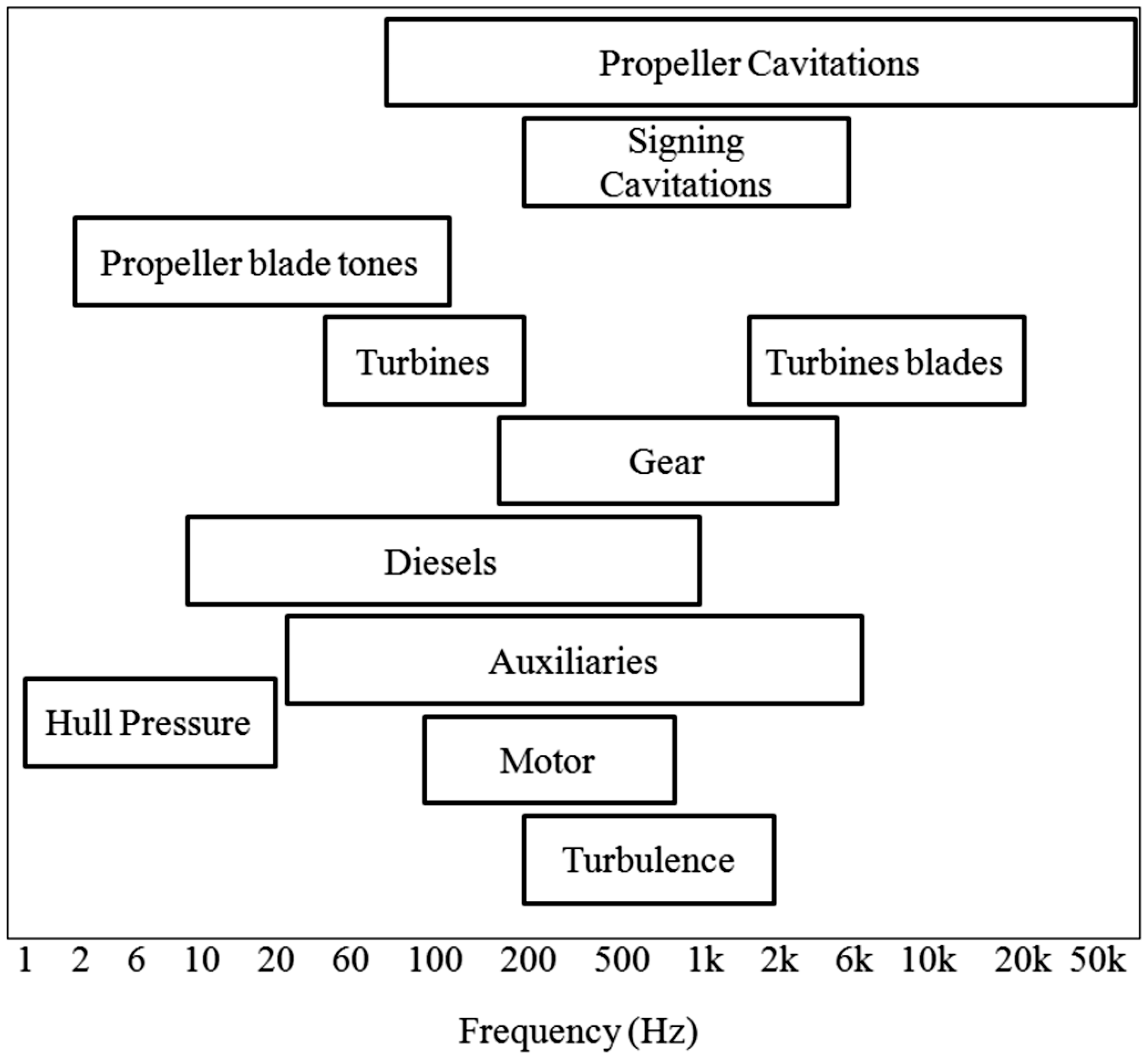
The range of underwater noise frequencies.²

Propeller noise can be classified into three categories: harmonic noise, broadband noise, and narrow-band random noise.

Harmonic noise is the periodic component, which can be represented by a pulse which repeats at a constant rate. Broadband noise is random in nature and contains components at all frequencies. Narrow-band random noise is almost periodic. However, examination of the harmonics reveals that the energy is not concentrated at isolated frequencies, but rather it is spread out. The mechanisms which lead to the generation of the spectral characteristics discussed above are described in four categories: steady sources, unsteady sources, random sources, and nonlinear effects.¹⁸

Steady sources appear constant in time to an observer on the rotating blade and produce periodic noise because of their rotation. Steady sources include three categories: linear thickness, linear loading, and (nonlinear) quadrupole.

Thickness noise arises from the transverse periodic displacement of the water by the volume of a passing blade element. The amplitude of this noise component is proportional to the blade volume, with frequency characteristics dependent on the shape of the blade cross section and rotational speed. Thickness noise can be represented by a monopole source distribution and becomes important at high speeds. Thin blade sections and plan form sweep are used to control this noise.¹⁹

Loading noise is a combination of thrust and torque (or lift and drag) components which result from the pressure field that surrounds each blade as a consequence of its motion. This pressure disturbance moving in the medium propagates as noise. Loading source can be represented by a dipole source and becomes an important mechanism at low to moderate speeds.

For moderate blade section speed, the thickness and loading sources are linear and act on the blade surfaces. For high-speed propeller, nonlinear effects can become significant. In hydroacoustic theory these sources can be modeled with quadrupole sources distributed in the volume surrounding the blades. In principle, the quadrupole could be used to account for all the viscous and propagation effects not covered by the thickness and loading sources. At high-speed blade section speeds the quadrupole enhances the linear thickness and loading sources and causes a noise increase for propellers.

Unsteady sources are time dependent in the rotating blade frame of reference. They include periodic and random variation of loading on the blades. For example, for a propeller behind an aft wake regardless of the number of blades on the propeller, the loading on the blade varies during a revolution. Unsteady loading is an important source in the counter-rotating propeller.

Unsteady random sources give rise to broadband noise. For propellers there are two sources which may be important, depending on the propeller design and operating conditions. The first broadband noise source is the interaction of inflow turbulence with the blade leading edges. Because the inflow is turbulent, the resulting noise is random. The importance of this noise source depends on the magnitude of the inflow turbulence, but it can be quite significant under conditions of high turbulence at low speeds.

In the second broadband mechanism, noise is generated near the blade trailing edge. A typical propeller develops a turbulent boundary layer over the blade surfaces, which can result in fluctuating blade loading at the trailing edge. The noise is characterized by the boundary layer properties. A related mechanism occurs at the blade tips, where turbulence in the core of the tip vortex interacts with the trailing edge. It has been determined for full-scale propellers that the broadband noise sources are relatively unimportant and do not contribute significantly to the total noise.¹⁸

Acoustic method based on the FW-H equation

The first and most accomplished research in acoustic waves has been done by Lighthill.²⁰ Two basic governing equations of the continuity and momentum are employed to obtain overall sound production relationship. By writing the continuity equation as follows

\frac{D ρ}{D t} + d i v (ρ \vec{u}) = \frac{\partial ρ}{\partial t} + \frac{\partial (ρ u_{i})}{\partial x_{i}} = q

(1)

where q is the mass production rate per unit volume. The momentum equation is expressed as

\frac{\partial (ρ u_{i})}{\partial t} + \frac{\partial (ρ u_{i} u_{j})}{\partial x_{i}} = - \frac{\partial p}{\partial x_{i}} - ρ g \frac{\partial τ}{\partial x_{i}} + f_{i}

(2)

where f_i represents the body forces. From equations (1) and (2), equation (3) is retrieved by the following form

\frac{\partial^{2} ρ}{\partial t^{2}} + c_{0}^{2} \nabla^{2} ρ = \frac{\partial^{2} (T_{i j})}{\partial x_{i} x_{j}}

(3)

Here, c₀ is the sound speed and T_ij is the Lighthill stress tensor. It is expressed as

T_{i j} = ρ u_{i} u_{j} + δ_{i j} (p - ρ c_{0}^{2}) + τ_{i j}

(4)

The first term on the RHS of equation (4) is the turbulence velocity fluctuations (Reynolds stresses), the second term is due to changes in pressure and density, and the third term is due to the shear stress tensor.

A generalization of Lighthill’s theory is to include hydrodynamic surfaces in motion. It is suggested by FW-H that has prepared the basis for an important amount of analysis of the noise caused by rotating blades, including propeller and fans. FW-H theory contains surface source terms in addition to the quadruple source. The surface sources are generally indicated as thickness (or monopole) sources and loading (or dipole) sources. This equation is presented as follows²¹

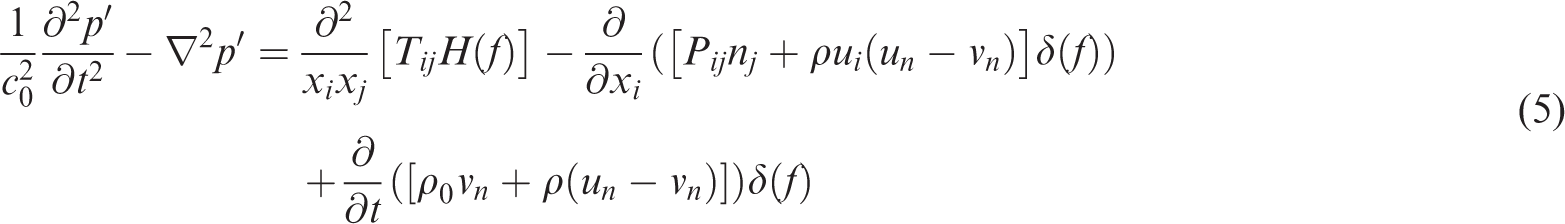
\begin{matrix} \frac{1}{c_{0}^{2}} \frac{\partial^{2} p^{'}}{\partial t^{2}} - \nabla^{2} p^{'} = \frac{\partial^{2}}{x_{i} x_{j}} [T_{i j} H (f)] - \frac{\partial}{\partial x_{i}} ([P_{i j} n_{j} + ρ u_{i} (u_{n} - v_{n})] δ (f)) \\ + \frac{\partial}{\partial t} ([ρ_{0} v_{n} + ρ (u_{n} - v_{n})]) δ (f) \end{matrix}

(5)

The terms at RHS are named quadruple, dipole, and monopole sources, respectively. p is the sound pressure at the far field ( $p^{'} = (p - p_{0})$ ). c₀ is the far-field sound speed and T_ij is the Lighthill stress tensor defined by equation (4). Also H(f) and δ(f) are Heaviside and Dirac delta functions, respectively. By solving this equation, pressure variation and SPL (measured in dB) are calculated by equation (6) as follows

S P L = 20 l o g_{10} \frac{P_{r m s}}{P_{r e f}}

(6)

where P_rms is the root mean square sound pressure and P_ref is the reference sound pressure, both measured in Pascals.

Numerical results and discussions

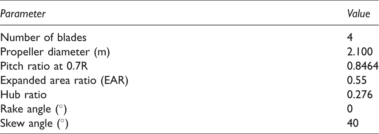
The propeller noise is calculated for comparison with the experimental results. The experimental data were carried out by Atlar et al.²² Main dimensions of the propeller are presented in Table 1. Incompressible finite volume method in commercial ANSYS Fluent 14.5 software is used.²³

Table 1.

Main dimensions of the propeller.

Parameter	Value
Number of blades	4
Propeller diameter (m)	2.100
Pitch ratio at 0.7R	0.8464
Expanded area ratio (EAR)	0.55
Hub ratio	0.276
Rake angle (°)	0
Skew angle (°)	40

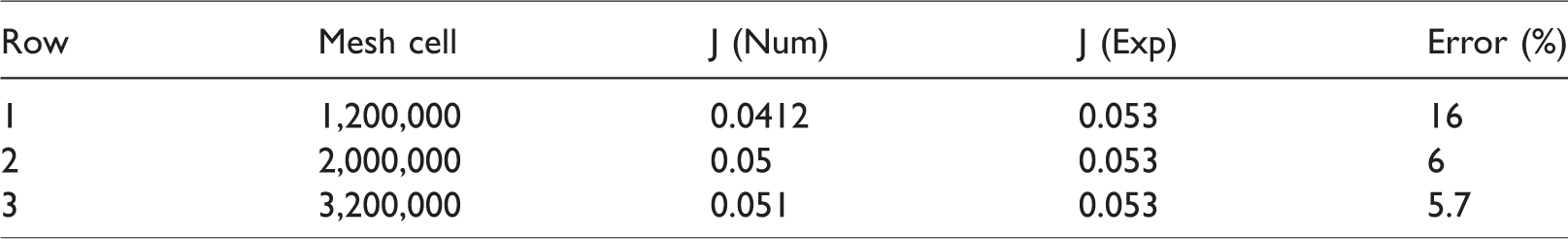
An unstructured hybrid mesh was applied for grid generation. Triangular cells are used for blades and hub surfaces. A fine grid was used for near wall to capture the flow in this region. The grid aspect ratio is gradually increasing to decrease solution costs. The study of grid independency for result validation was carried out in J = 0.74 and the results are presented in Table 2. It is shown that the second configuration has a best efficiency in the prediction of thrust coefficient and computational costs.

Table 2.

Grid independency and computational effort (J = 0.74).

Row	Mesh cell	J (Num)	J (Exp)	Error (%)
1	1,200,000	0.0412	0.053	16
2	2,000,000	0.05	0.053	6
3	3,200,000	0.051	0.053	5.7

A moving reference frame was used to generate rotational speed around propeller. The generated grid is shown in Figure 2.

Figure 2.

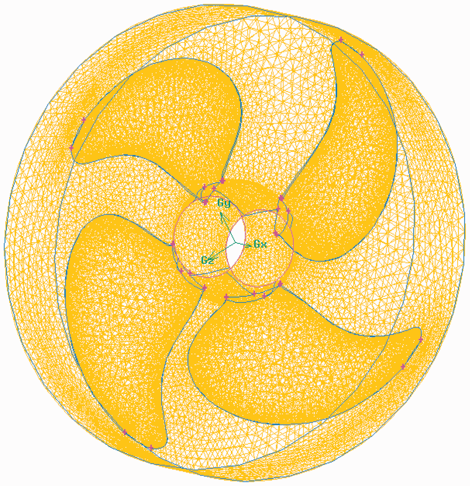
The generated unstructured grid on propeller.

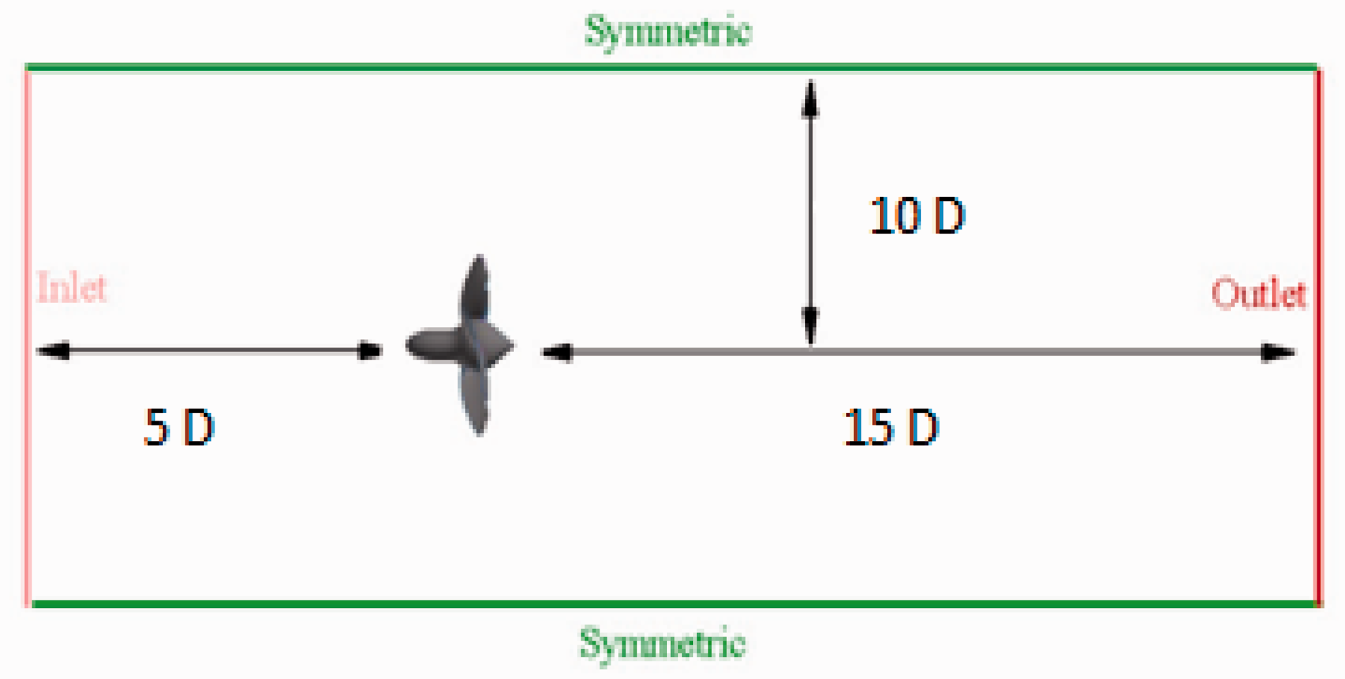
Computational domain is defined at 5D for upstream, 15D at downstream, and 10D for side one (D is propeller diameter). About two million cells have been created for whole domain grid, as demonstrated in Figure 3.

Figure 3.

The generated unstructured grid on propeller.

In order to study the propeller performance in uniform flow and applying open water condition, a rectangular control volume was considered around the propeller with velocity inlet and pressure outlet boundary conditions. The domain distances were considered large sufficiently to keep away from blockage effects on the propeller hydrodynamic performance characteristics.

The SIMPLE algorithm is used for pressure–velocity coupling equation and second-order upstream discretization for momentum equations. Realizable k–ε model is used to model turbulence with time step equal to 1e-4. To capture sound, the receivers are adjusted in four points above the propeller at z-axis (z/D = 0.5, 1, 1.5, 2) and also at four points downstream locations (x/D = 0.5, 1, 1.5, 2) from center of the propeller as shown in the coordinate system of the propeller in Figure 4.

Figure 4.

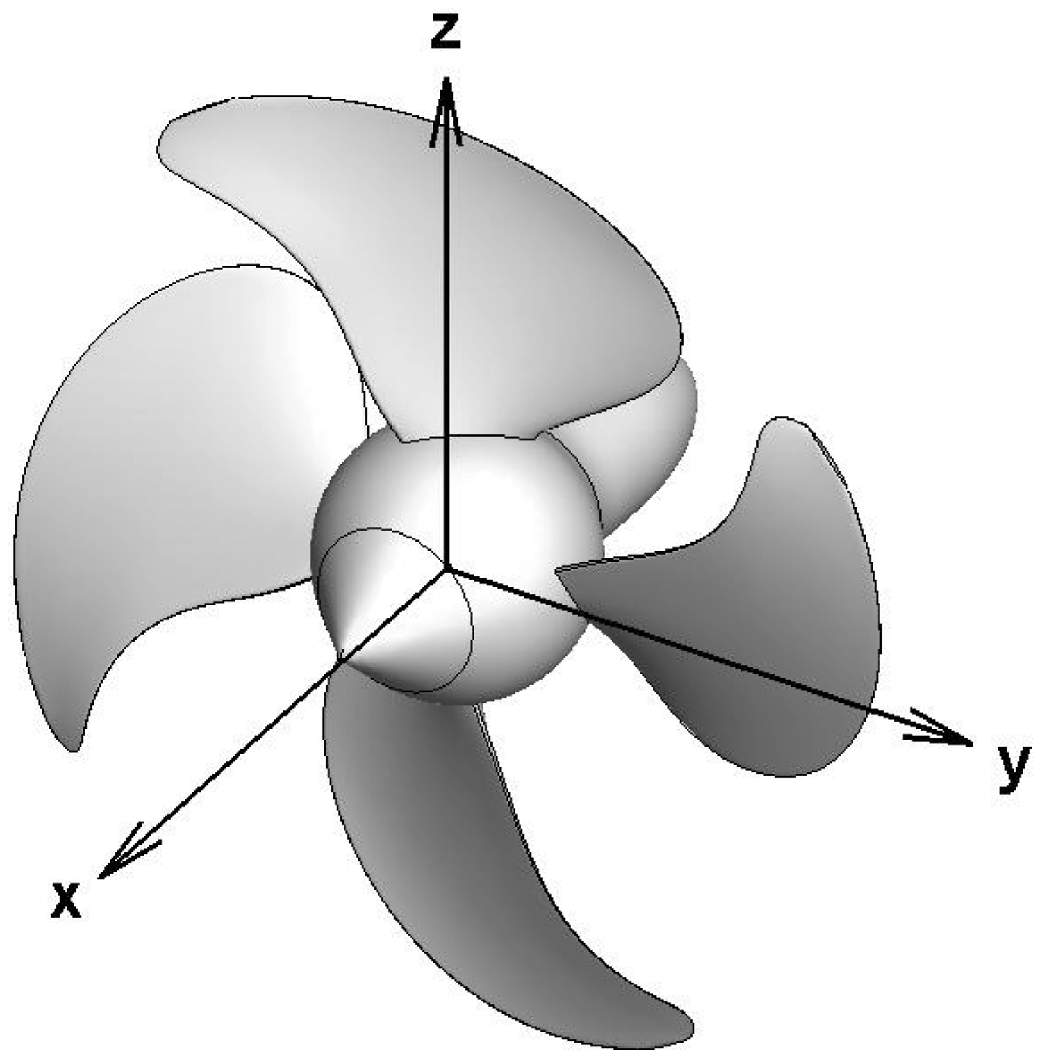
Coordinate system of the propeller.

Figure 5 shows the wake distribution which displayed excellent wake uniformity due to the stern form.

Figure 5.

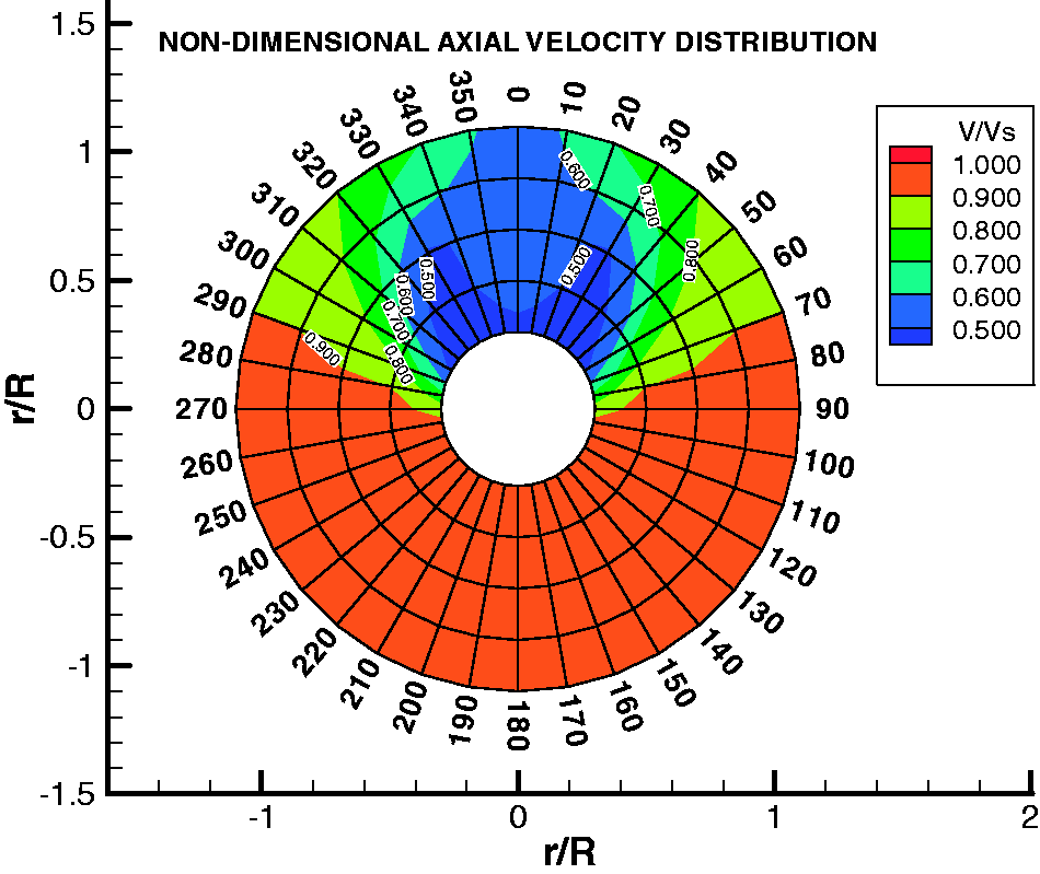
Nonuniform wake field in terms of velocity ratios.¹⁷

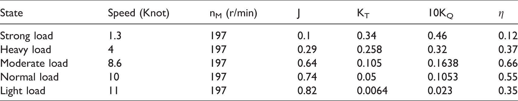
First of all, for better understanding, the pressure distributions on the propeller and other locations are shown. Pressure contour on the propeller blade surfaces (back and front) at normal and heavy load conditions is shown in Figures 6 and 7, respectively. At heavy loads (low advance ratios) the difference between pressures coefficients on both sides of the propeller increases significantly, while at light load condition the pressure difference is relatively low.

Figure 6.

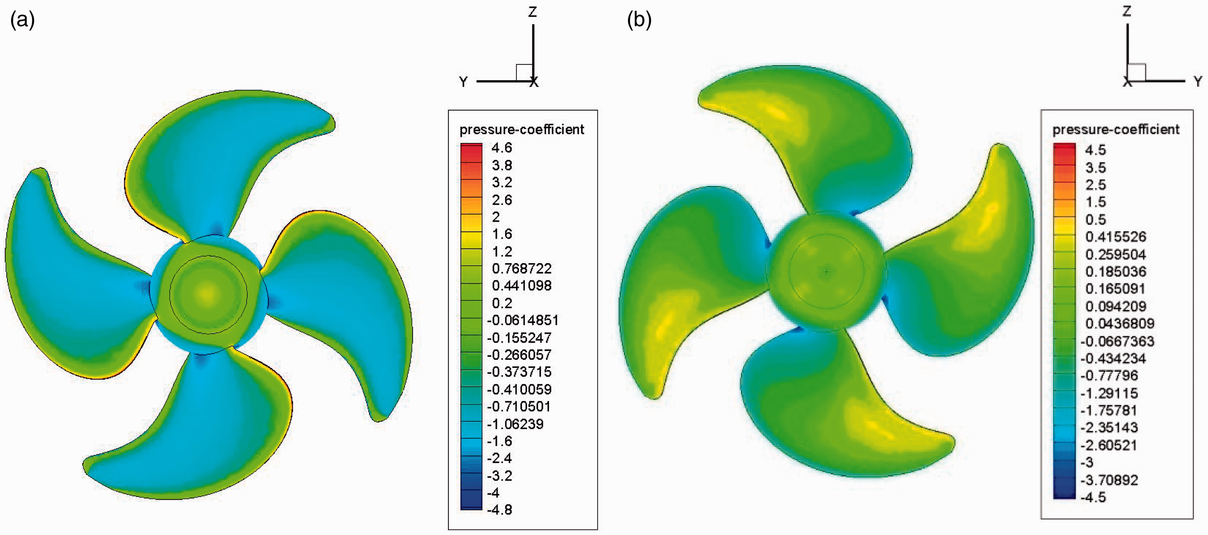
Pressure coefficient distribution on normal load condition (a) pressure side and (b) suction side.

Figure 7.

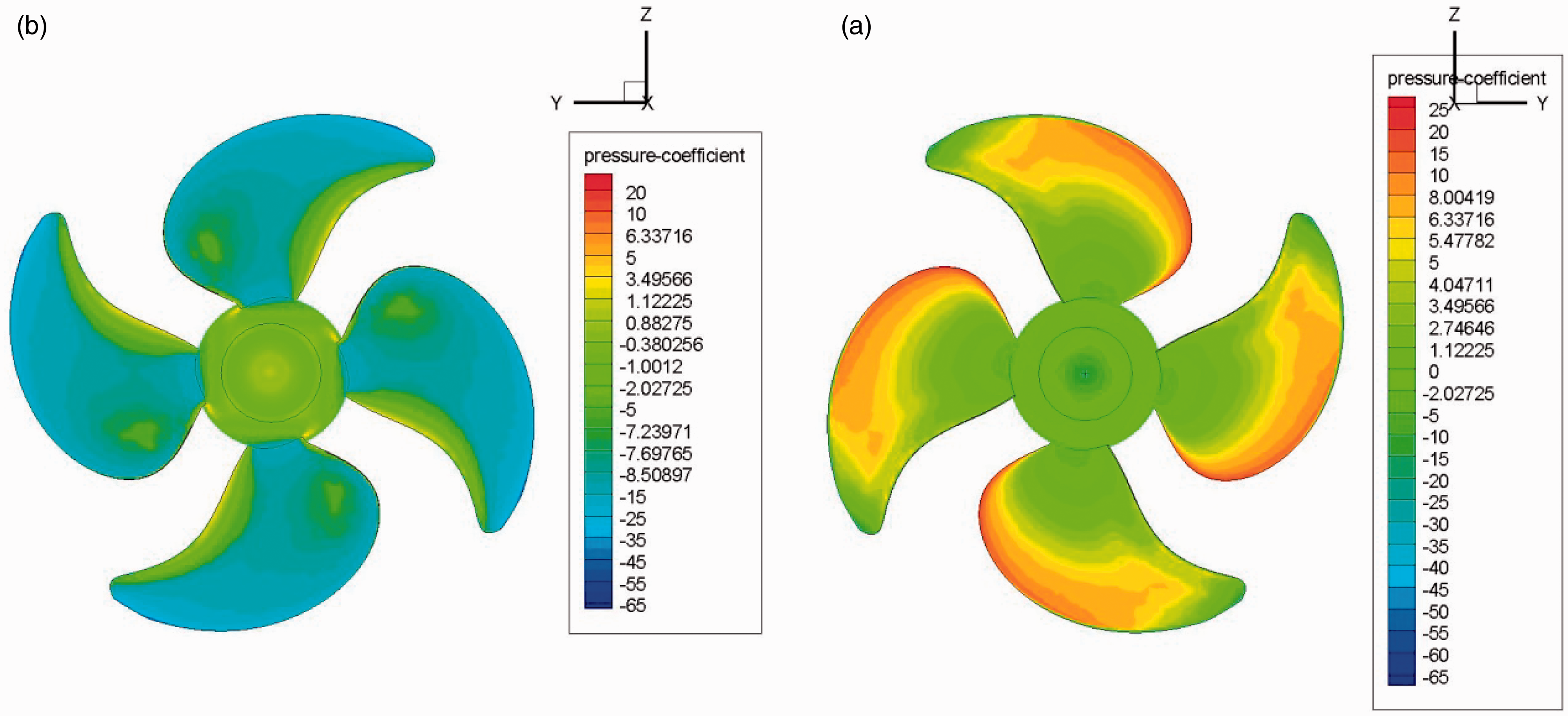
Pressure coefficient distribution on heavy load condition: (a) pressure side and (b) suction side.

Also, the pressure coefficient results for back and front are shown in Figures 8 and 9 at four radial sections (r/R = 0.3, 0.5, 0.7, 0.9) on the blade. By comparing Figure 8(a) to (d), it is concluded that the difference between the pressure coefficients is much greater on the far sections (c) and (d) with respect to near sections (a) and (b). In addition, range of the pressure coefficient of heavy load propeller is much greater than the normal load propeller, which shows more thrust at low advance ratios.

Figure 8.

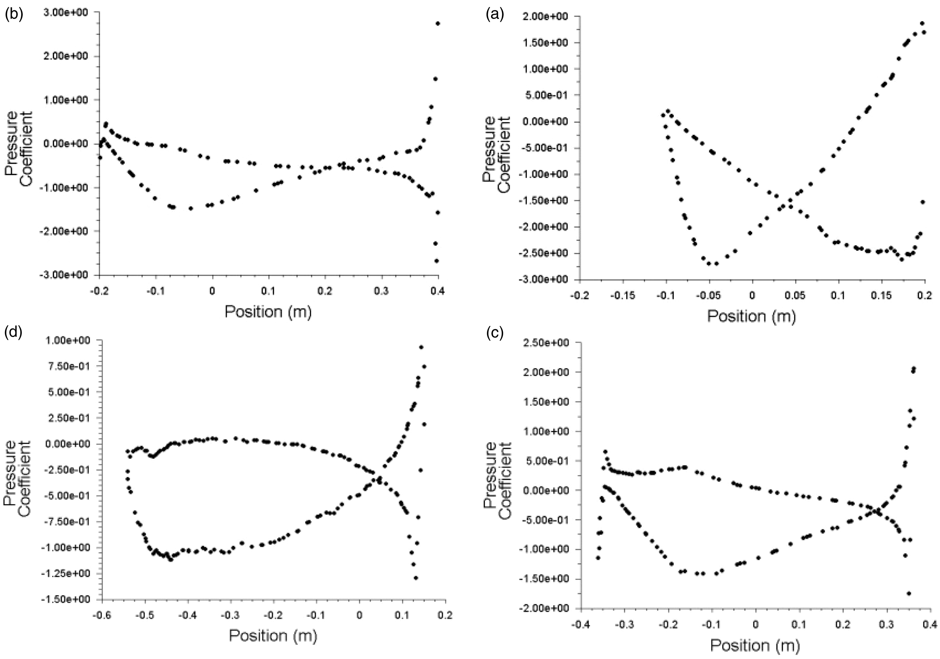
Pressure coefficient distribution on blade section for normal load condition. (a) r/R=0.3, (b) r/R =0.5, (c) r/R =0.7, and (d) r/R=0.9.

Figure 9.

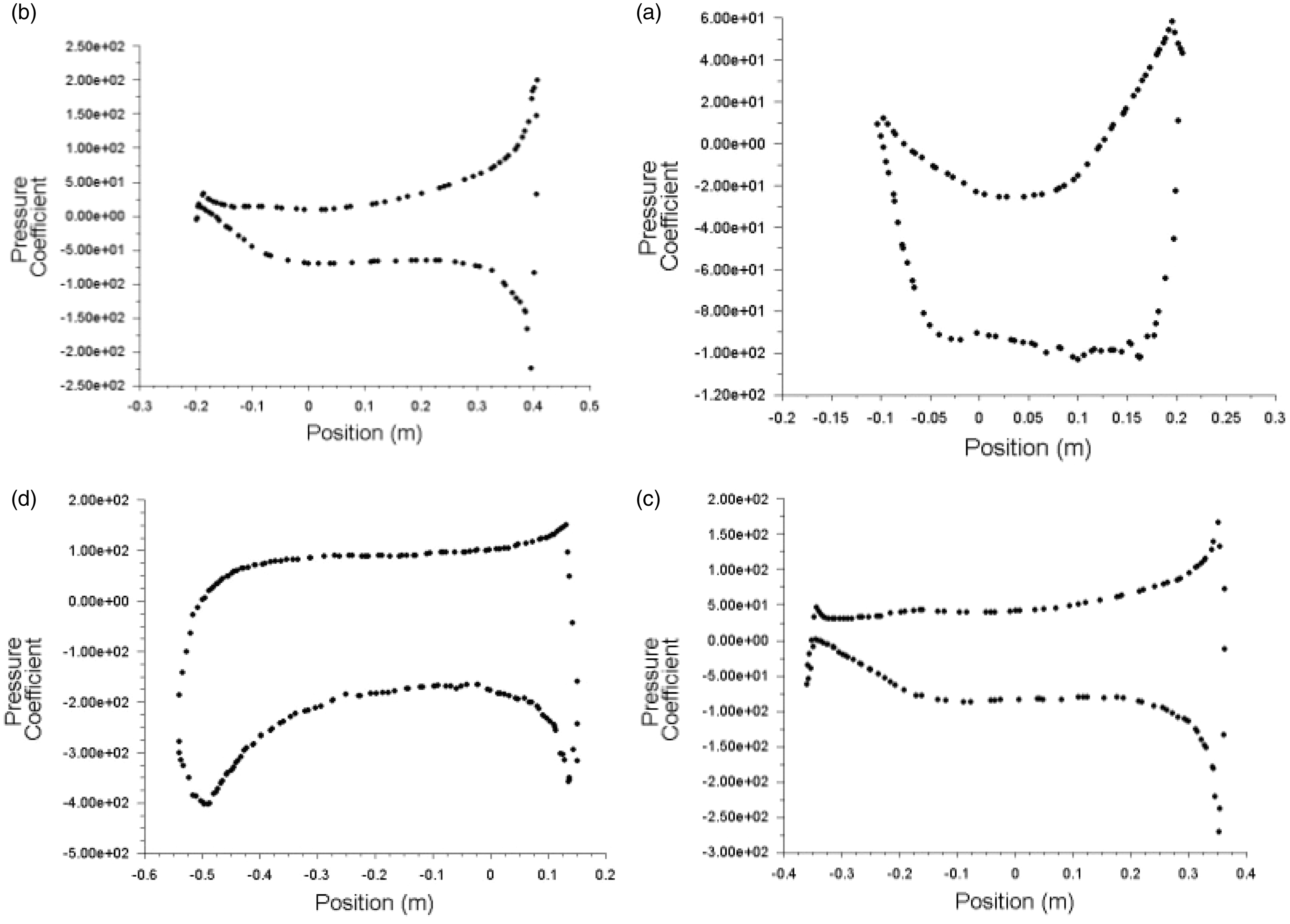
Pressure coefficient distribution on blade section for heavy load condition. (a) r/R = 0.3, (b) r/R =0.5, (c) r/R =0.7, and (d) r/R = 0.9.

Hydrodynamic characteristics of the propeller at various operating conditions are shown in Figure 10 and compared with experimental data.²² Efficiency is low for heavy load condition and when it becomes light condition the efficiency increases.

Figure 10.

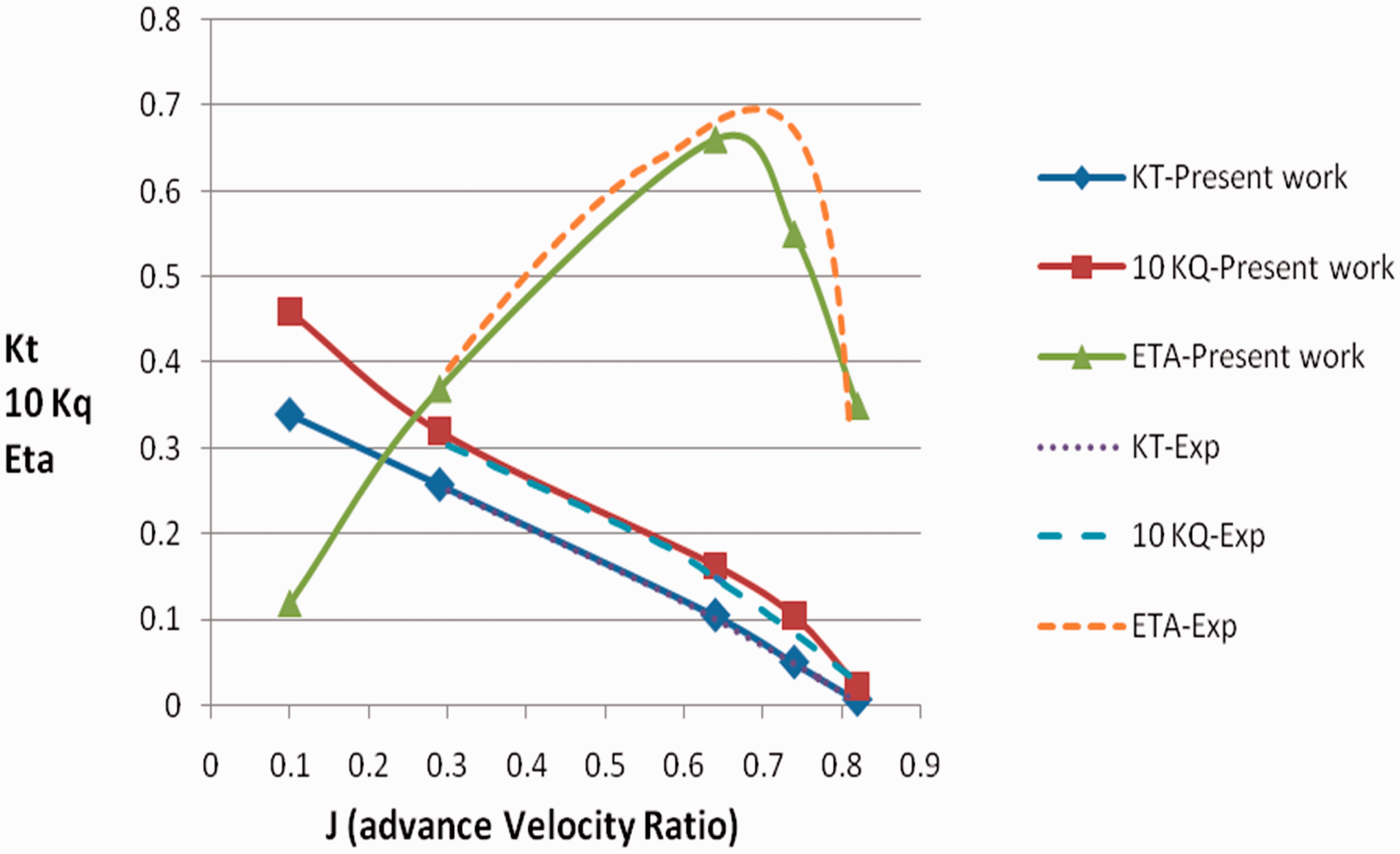
Hydrodynamic characteristics of the propeller.

Also, Table 3 presents more details at five operating conditions (propeller speed and advance velocity) and its hydrodynamic performance. Propeller rotating speed is constant (197 r/min) while advance speed is changed from 1.3 to 11 knots. Advance velocity ratio is from 0.1 (heavy condition) to 0.82 (light condition). The maximum efficiency is obtained about 66%.

Table 3.

Hydrodynamic characteristics results at five operating conditions.

State	Speed (Knot)	n_M (r/min)	J	K_T	10K_Q	η
Strong load	1.3	197	0.1	0.34	0.46	0.12
Heavy load	4	197	0.29	0.258	0.32	0.37
Moderate load	8.6	197	0.64	0.105	0.1638	0.66
Normal load	10	197	0.74	0.05	0.1053	0.55
Light load	11	197	0.82	0.0064	0.023	0.35

Pressure coefficient distribution for normal and heavy load condition is shown in Figure 11. Maximum pressure happens at the blade tip and pressure side. Minimum pressure occurs at the blade root and back surface. Also there is a pressure drop region in downstream.

Figure 11.

Contour of the pressure coefficient distribution for normal and heavy load condition in downstream.

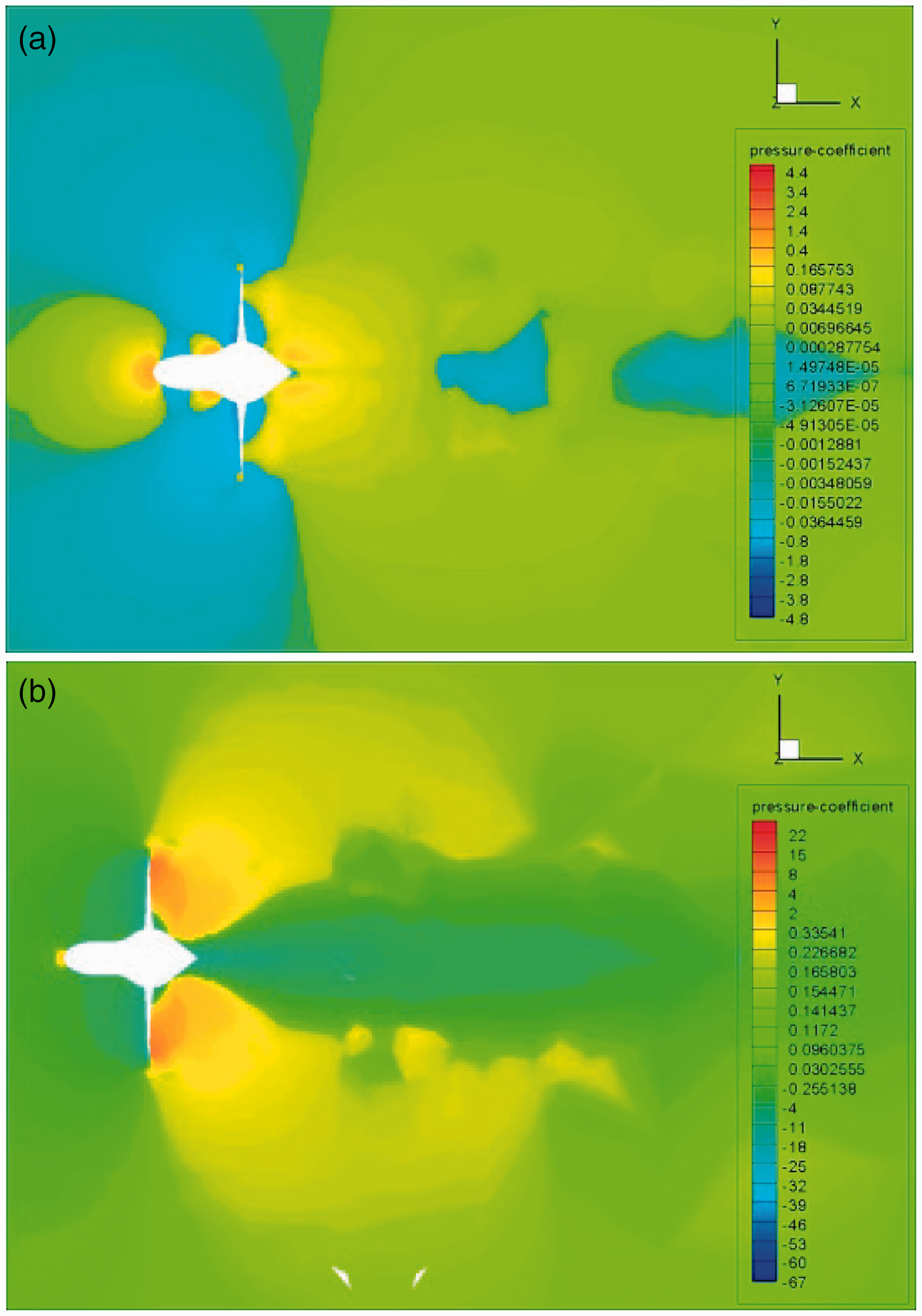
Figure 12 illustrates two views of distribution axial velocity, where propeller is rotating with a constant rotational velocity of 197 r/min. The figure shows the flow field in which blade tip produces high-speed backward flow (regions marked red). At the same time a forward flow with lower axial velocity is also generated. These two reverse flows stimulate a vertical flow around the blade tip.

Figure 12.

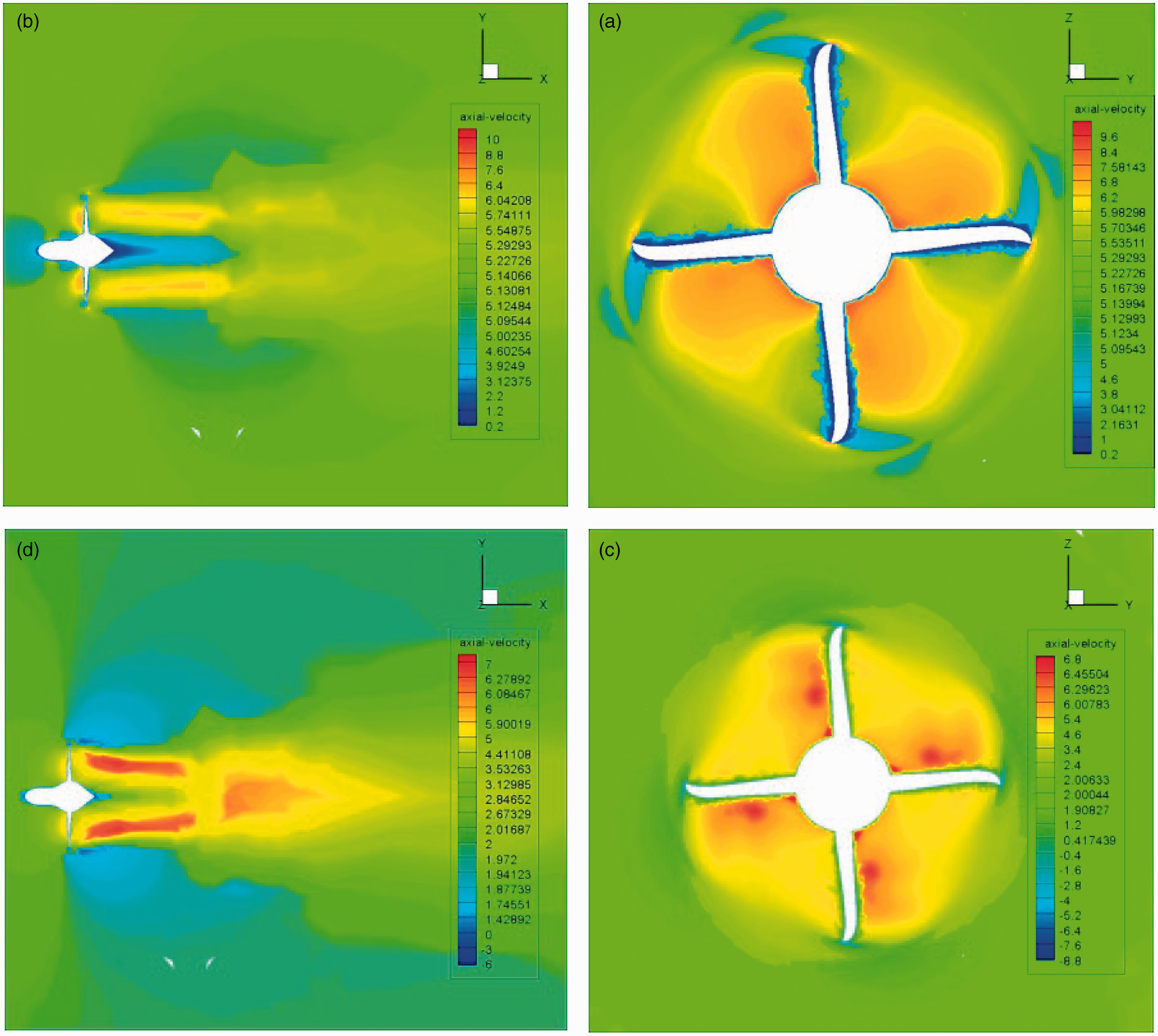
Contour of the axial velocity distribution in blade section and downstream for (a, b) normal load condition and (c, d) heavy load condition.

SPL around propeller

In the previous section, the accurate explanation of the flow around the propeller was obtained that produces noise sources. With provided source component, acoustic analogy approximation can be used to assess the numerical broadband noise. The density and sound speed in water are $ρ = 1, 000 kg / m^{3}$ and 1480 m/s. The reference pressure for SPL is 1.0 µPa.

Numerical calculations of the SPL and experimental data are compared at z/D = 1.5 for normal load condition as shown in Figure 13. There is a good agreement between the numerical and experimental results. In this diagram for estimated frequency 80 Hz, the peak noise level equal to 143 dB is obtained. Noise at frequencies between 1000 and 3000 drop to 100 dB.

Figure 13.

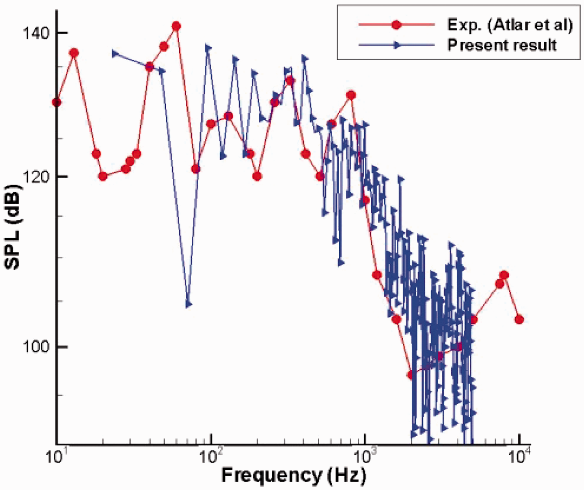
Comparison of the SPL at normal load condition and z/D = 1.5. SPL: sound pressure level.

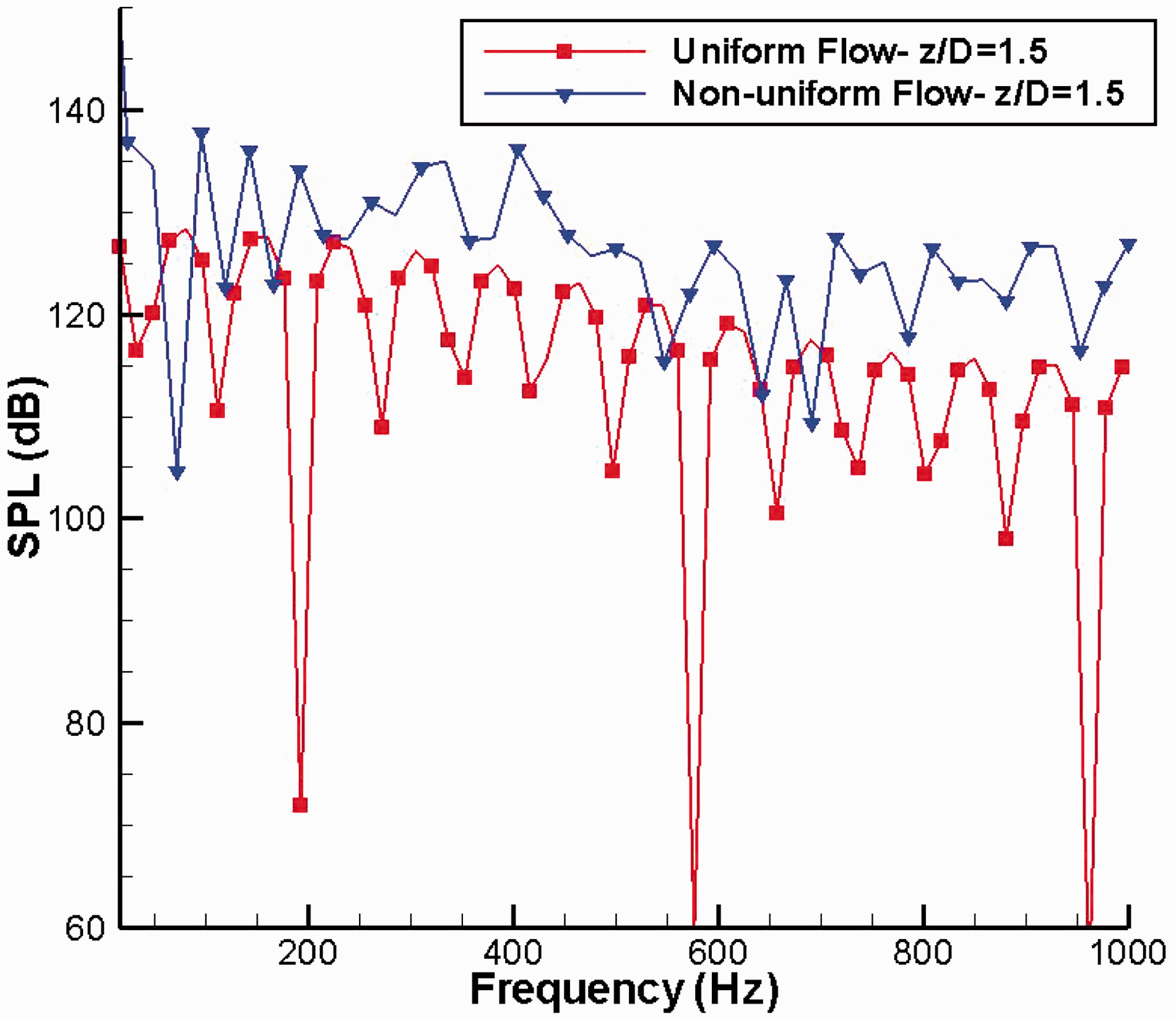
Also the comparison between noise spectrum uniform and nonuniform flow for x/D = 0.5, x/D = 1.5 and z/D = 0.5, z/D = 1.5 is illustrated in Figures 14 to 17. The SPL for nonuniform flow is around 10% greater than uniform flow.

Figure 14.

Comparison of the SPL at uniform and nonuniform flows for normal load (x/D = 1.5, J = 0.74). SPL: sound pressure level.

Figure 15.

Comparison of the SPL at uniform and nonuniform flows for normal load (x/D = 1.5, J = 0.74). SPL: sound pressure level.

Figure 16.

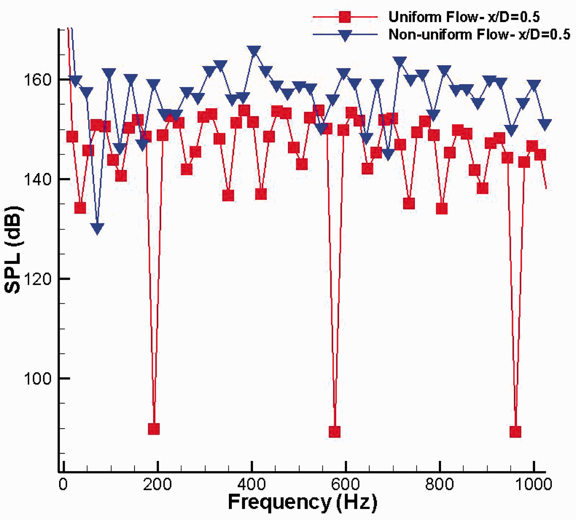
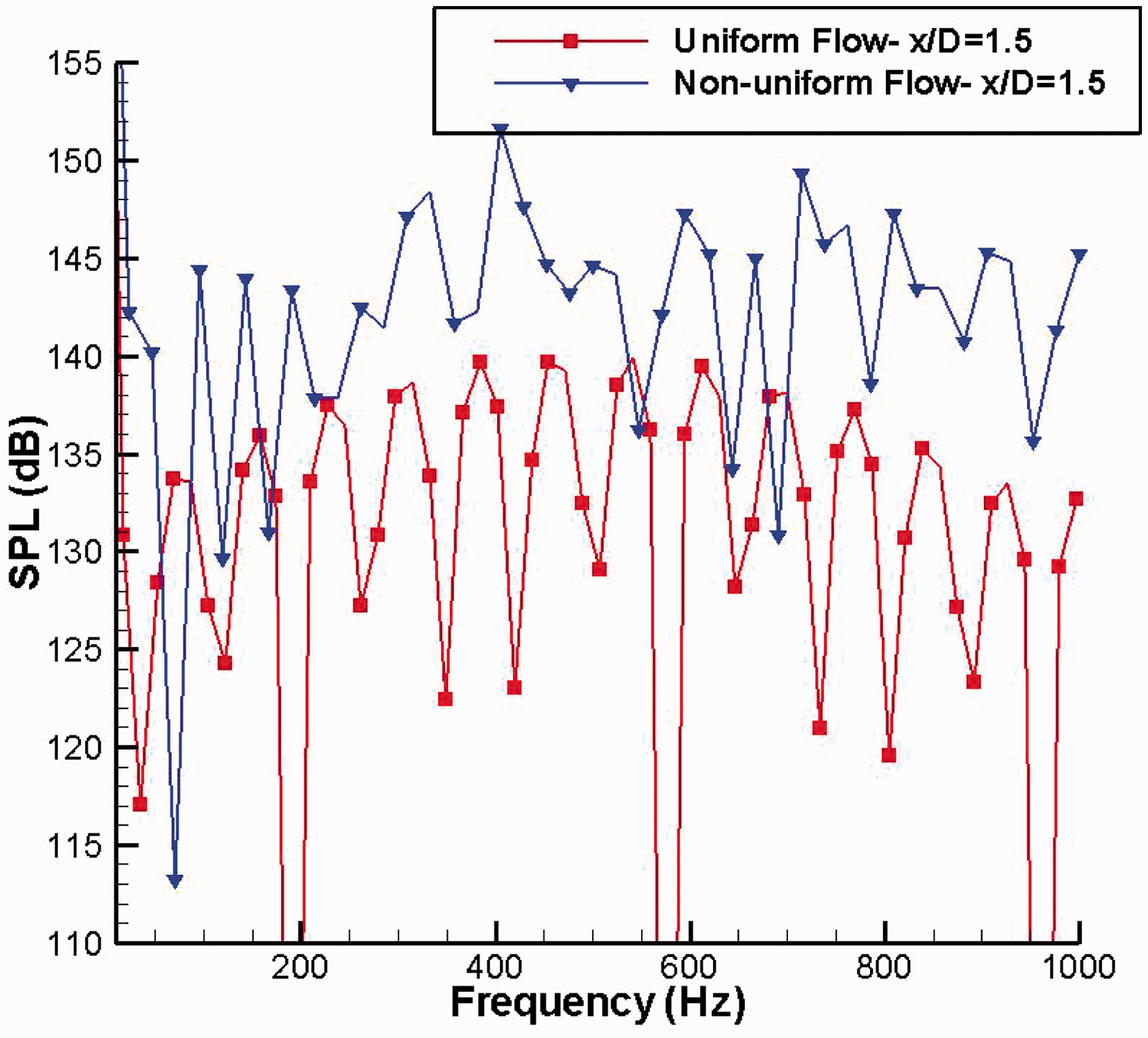
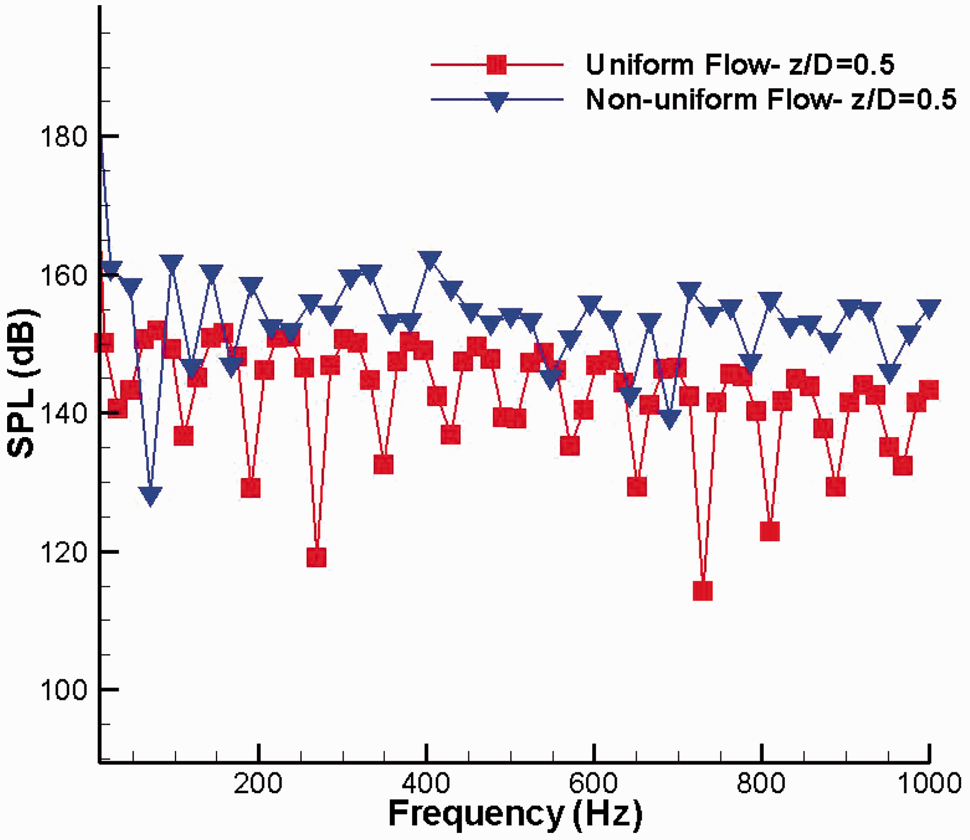
Comparison of the SPL at uniform and nonuniform flows for normal load (z/D = 1.5, J = 0.74). SPL: sound pressure level.

Figure 17.

Comparison of the SPL at uniform and nonuniform flows for normal load (z/D = 1.5, J = 0.74). SPL: sound pressure level.

The tonal peaks at multiples of the BPF can be observed obviously on the spectrum plat. (f = 17, 34, 68, 136,… Hz).

In order to equal rotational speed in these two conditions, thickness noise is equal in both but the difference is caused by the addition of loading noise (dipole) source due to nonuniform flow.

As shown, the overall SPL decreases as the distance from the sound source raises. In the far field where sound propagates as spherical waves and kr ≫ 1(k is the wave number and r is the distance to sound source) sound pressure follows the inverse square law with respect to the distance. This means that, in the far field, the overall SPL is identified with the reverse square of the distance. For instance, if the distance doubles the overall SPL reduces around 6–7 dB. As discussed, this comment uses to predict the proper magnitude just for the far field. As shown in this figure, SPL for z/D = 0.5 and z/D= 1.5 is varied about 20 dB.

Conclusions

In order to estimate the propeller low frequency noise spectrum, a test case model was introduced and various investigations have been done on this sample test. Pressure distribution and hydrodynamic characteristics of the propeller are determined at various operating conditions. SPLs are presented at downstream as well as above the propeller. Numerical results are in good agreement with the experimental data. The SPL has been figured to be fairy complex due to the complicated physics of viscous influence and vortex manner in the flow above propeller blades. The sound is produced by the Lighthill tensor, the oscillating force, and the torque. Based on the numerical results, the sounn level at uniform flow has some jump points, but it is almost smooth at non-uniform flow.

Footnotes

Declaration of conflicting interests

The author(s) declared no potential conflicts of interest with respect to the research, authorship, and/or publication of this article.

Funding

The author(s) received no financial support for the research, authorship, and/or publication of this article.

References

Ravindra

Brijendra

and Ayaz

JK.

A theoretical investigation of natural frequencies of vibration and noise due to engine and propeller systems of an ultra large crude carrier (ULCC). J Low Freq Noise Vib Active Control 2010; 29: 41–53.

Carlton

JS.

Marine propeller and propulsion. 3rd ed., Elsevier publication, 2013.

Crocker

MJ.

Encyclopedia of acoustics. John Wiley publication, 1997.

and Huang

Research on the mechanism of fan blade shape effect on its noise. J Low Freq Noise Vib Active Control 2005; 24: 59–70.

Madsen

HA.

Low frequency noise from wind turbines mechanisms of generation and its modelling. J Low Freq Noise Vib Active Control 2010; 29: 239–251.

Pan

YC and

Zhang

HX.

Numerical hydro-acoustic prediction of marine propeller noise. J Shanghai Jiaotong Univ (Sci) 2010; 15: 707–712.

Kerwin

JE and

Lee

CS.

Prediction of steady and unsteady marine propeller performance by numerical lifting-surface theory. Soc Naval Architects Mar Eng Trans 1978; 86: 218–253.

Hoshino

Hydrodynamic analysis of propeller in unsteady flow using a surface panel method. J SNAJ Nihon Zousen Gakkai Ronbunshu 1993; 74: 71–87.

Funeno

Analysis of unsteady viscous flows around a highly skewed propeller. J Kansai Soc Naval Architects 2002; 237: 39–45.

10.

Huang

ZY and

Hong

FW.

Unsteady hydrodynamics forces of propeller predicted with viscous CFD. J Hydrodyn 2009; 24: 734–739.

11.

W and

Yang

Numerical simulation of flow around a podded propeller. In: Proceedings of the 19th international offshore and polar engineering conference, Osaka, Japan, 2100–26 July 2009.

12.

Kheradmand

Rahrovi

A and

Mousavi

Numerical simulation of tonal and broadband hydrodynamic noises of noncavitating underwater propeller. Polish Maritime Res 2014; 21: 46–53.

13.

Seol

Suh

JC and

Lee

Development of hybrid method for the prediction of underwater propeller noise. J Sound Vib 2005; 288: 345–360.

14.

Park

Seol

Choi

et al . Numerical prediction of tip vortex cavitation behaviour and noise considering nuclei size and distribution. Appl Acoustics 2009; 70: 674–680.

15.

Seol

Jung

Suh

et al . Prediction of non-cavitating uunderwater propeller noise. J Sound Vib 2002; 257: 131–156.

16.

Wang

Marsden

AL and

Moin

Computation and control of trailing-edge noise. In: Proceedings of the 26th symposium on naval hydrodynamics, Rome, Italy, 2006.

17.

Jang

Kim

HT and

Joo

WH.

Numerical study on non-cavitating noise of marine propeller. In: Inter.noise, Melbourne, Australia, 16–19 November 2014.

18.

Caridi

Industrial CFD simulation of aerodynamic noise . PhD Thesis, Napoli University, 2007.

19.

Ross

Mechanics of underwater noise. Los Altos, CA: Peninsula Publishing, 1987, p.322.

20.

Lighthill

MJ.

On sound generated aerodynamically, І. General theory. In: Proceedings of the Royal Society of London, London, 20 March 1952.

21.

Williams

JE and

Hawkings

DL.

Sound generated by turbulence and surfaces in arbitrary motion. Phil Trans R Soc 1969; 264: 321–342.

22.

Atlar

Takinacı

Korkut

et al . Cavitation tunnel tests for propeller noise of a FRV and comparisons with full-scale measurements. In: Fourth international symposium on cavitation, Pasadena, USA, 20–23 June 2001.

23.

ANSYS Fluent Release 14.5, Solver theory documentation, predicting aerodynamically generated noise, 2012.

Calculation of sound pressure level of marine propeller in low frequency

Abstract

Keywords

Introduction

Wide range of frequencies of the propeller noise

Acoustic method based on the FW-H equation

Numerical results and discussions

SPL around propeller

Conclusions

Footnotes

Declaration of conflicting interests

Funding

References