Sage Journals: Discover world-class research

Abstract

A two-dimensional boundary element method with a constant element type was adopted to study the sound field of a building near a roadway. First, a factor analysis of the computed results has been done, which include the element length, the Hankel functions’ calculation accuracy, and numerical integration accuracy. Then, boundary element method is applied to calculate building attenuation with different building aspect ratios and different frequencies with balconies, followed by drawing of the sound field distribution diagram. The calculation results revealed the following: (1) a wider building results in a more severe sound attenuation; (2) balconies on different floors produce a reduction of approximately 15 dB for broadband spectral characteristics of A-weight road traffic noise, and the maximum values appear at the bottoms of balconies; (3) for the points in the balconies, higher sound frequencies are correlated to larger insertion loss, with the insertion loss increasing from 3 dB to >10 dB when the sound frequency increases from 20 to 4000 Hz; (4) calculations of three typical frequencies indicate that the insertion loss of 500 Hz (main frequency of heavy vehicles) is 6 dB less than that of 800 Hz (main frequency of light vehicles), i.e. the flow control of heavy vehicles could conspicuously improve the ambient acoustic environment of buildings near a roadway.

Keywords

Building nearby roadway boundary element method insertion loss balconies sound frequency

Introduction

The phenomenon of the propagation of sound waves around obstacles is one important form of sound transmission. Of particular interest are the acoustic environments of the buildings close to roadways because they have a direct effect on our daily lives.^1,2 Nowadays, scholars have proposed numerous methods to calculate the acoustic attenuation, which include the experimental modeling method,^3,4 the geometrical acoustics method,^5,6 and the numerical simulation method.^7–9 The experimental modeling method produces scene-adaptive models that generate results that more closely approximate the real sound pressure level (SPL). However, the method is limited in use as it requires substantial equipment and manpower. The geometrical acoustics method, such as the geometrical theory of diffraction (GTD),¹⁰ the ray tracing method,^11,12 the beam tracing method,^13–15 the image source method,¹⁶ and comprehensive methods,^17,18 can model the reflection and diffraction effects by simulating the traces of sound. While, such modeling demands strict control¹⁹ over the many calculation parameters and can be very computationally intensive when the process of sound transmission is complex.²⁰ In addition, relatively small dimensions limit the accuracy of these methods for low-frequency sound transmission calculation. Another common and effective simulation method that is widely used is the numerical simulation method, which includes the boundary element method (BEM),^21–24 finite element method,^25–28 and finite difference method.^29,30 In this method, reflection and diffraction are not considered separately but appear as an integral part of the solution of the wave equation. Due to the advantages of dimensionality reduction, high calculation accuracy and excellent adaptability to complex boundaries,³¹ BEM has been used to calculate the reactions to noise by the various shapes of barriers,³² balconies,³³ and buildings³⁴ of a typical region.

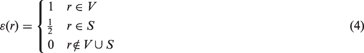
The purpose of the work is to investigate the sound field of a building region produced by a nearby stream of road traffic via BEM, which persuade three objectives. First, it can provide noise distribution of balconies building area instead of only typical points, and the noise analysis based on this can be not only global but also local. Second, discussions of accuracy analytical solutions, considering frequencies of traffic noise, were also introduced. Third, balconies, different aspect ratios, and various frequencies are considered to describe the properties of sound attenuation of the building region, with a focus on balconies. In addition, simple measures are considered for noise abatement.

BEM equations for sound fields

Establishment of the boundary integral equation

As shown in Figure 1, there is a two-dimensional (2D) sound field involving a long enough sound barrier and a line acoustic source which is parallel to both the sound barrier and the ground. S is taken as the boundary of the sound barrier, the acoustic source is located at r₀ = (x₀, y₀), an arbitrary receiving point is located at r = (x, y), the sound pressure p(r, r₀) at r satisfies the equation

(\nabla^{2} + k^{2}) p (r, r_{0}) = δ (r - r_{0})

(1)

where

\nabla^{2} = \frac{\partial^{2}}{\partial x^{2}} + \frac{\partial^{2}}{\partial y^{2}}

is the Laplace operator;

k = \frac{ω}{c}

is the wave number, ω is the wave frequency, c is the sound velocity, and

δ (r - r_{0})

represents the sound source at r₀.

Figure 1.

A two-dimensional sound field.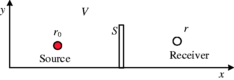

On the boundary, p(r, r₀) satisfies the impedance boundary conditions

\frac{\partial p (r, r_{0})}{\partial n} = ik β (r) p (r, r_{0})

(2)

where n is the outward normal direction of the boundary, i stands for the imaginary unit, and β refers to the acoustic admittance of the boundary.

A boundary integral equation can be obtained according to Green’s second integral formula, considering conditions of the boundary and properties of the δ function

ɛ (r) p (r, r_{0}) = G_{β c} (r, r_{0}) + \int_{S} p (r, r_{0}) (\frac{\partial G_{β c} (r_{s}, r)}{\partial n} - ik β (r_{s}) G_{β c} (r_{s}, r)) d S

(3)

where

\begin{matrix} ɛ (r) = {\begin{matrix} 1 & r \in V \\ \frac{1}{2} & r \in S \\ 0 & r \notin V \cup S \end{matrix} \end{matrix}

(4)

where G_βc(r, r₀) is a fundamental solution of the Helmholtz equation, suppose the ground is a fully rigid boundary, then G_βc(r, r₀) can be expressed as

G_{β c} (r, r_{0}) = - \frac{i}{4} [H_{0}^{(1)} (k | r - r_{0} |) + H_{0}^{(1)} (k | r - r'_{0} |)]

(5)

here

r'_{0} = (x_{0}, - y_{0})

stands for the mirror image source of r₀ relative to the ground;

H_{0}^{(1)}

is a zero-order Hankel function of the first kind.

BEM used to solve boundary integral equations

Divide the boundary S discretely into N small linear elements and mark them s₁, s₂,…s_N. Let the SPL p(r_i, r₀) at the midpoint of element i denote the sound pressure at any point within the element, then equation (3) can be written as

ɛ (r) p (r, r_{0}) = G_{β c} (r, r_{0}) + \sum_{i = 1}^{N} p (r_{i}, r_{0}) \int_{s_{i}} [\frac{\partial G_{β c} (r_{s_{i}}, r)}{\partial n} - ik β (r_{s_{i}}) G_{β c} (r_{s_{i}}, r)] d s_{i}

(6)

r is set as r_1, r_2, …, r_N, then a group of coefficient linear equations could be obtained, with respect to unknowns of p(r₁, r₀), p(r₂, r₀), …, p(r_N, r₀)

[A] [P] = [G]

(7)

where

\begin{matrix} [A] = [\begin{matrix} a_{1, 1} & a_{1, 2} & \dots & a_{1, N} \\ a_{2, 1} & a_{2, 2} & \dots & a_{2, N} \\ : & : & : \\ a_{N, 1} & a_{N, 2} & \dots & a_{N, N} \end{matrix}] \end{matrix}

(8)

\begin{matrix} a_{i, j} = {\begin{matrix} \int_{s_{j}} [\frac{\partial G_{β c} (r_{s_{j}}, r_{i})}{\partial n} - ik β (r_{s_{j}}) G_{β c} (r_{s_{j}}, r_{i})] - ɛ (r_{i}) & i = j \\ \int_{s_{j}} [\frac{\partial G_{β c} (r_{s_{j}}, r_{i})}{\partial n} - ik β (r_{s_{j}}) G_{β c} (r_{s_{j}}, r_{i})] & i \neq j \end{matrix} \end{matrix}

(9)

[P] = [\begin{matrix} p (r_{1}, r_{0}) & p (r_{2}, r_{0}) & \dots & p (r_{N}, r_{0}) \end{matrix}]^{T}

(10)

[G] = [\begin{matrix} - G_{β c} (r_{1}, r_{0}) & - G_{β c} (r_{2}, r_{0}) & \dots & - G_{β c} (r_{N}, r_{0}) \end{matrix}]^{T}

(11)

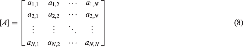
All elements in matrix [A], vector [P], and vector [G] are complex ones. Solve the linear equations, and put the obtained boundary sound pressure p(r₁, r₀), p(r₂, r₀), … , p(r_N, r₀) into equation (6), then sound pressure p(r, r₀) can be calculated.

Then ΔL, the insertion loss of the sound barrier, is given by the following formula

Δ L = 20 \lg \frac{| p_{0} (r, r_{0}) |}{| p (r, r_{0}) |}

(12)

where p₀(r, r₀) stands for the sound pressure at the receiving point if the sound barrier takes no effect

p_{0} (r, r_{0}) = - \frac{i}{4} [H_{0}^{(1)} (k | r - r_{0} |) + H_{0}^{(1)} (k | r - r'_{0} |)]

(13)

A factor analysis of the computed results

Impact of the element length

During the calculation of the building’s insertion loss ΔL using BEM, the precision and the calculation efficiency of the final result can be affected by the element length. There have been many studies on analysis of element size in BEM. As such, Marburg and Schneider,³⁵ Marburg,³⁶ Nolte and Marburg,³⁷ and some others presented and discussed formulation of discontinuous elements and position of nodes on the element. A 2D building, depicted in Figure 2(a), was used as an example to study the effects of the element length on results of BEM. The acoustic absorptivity of building is 0.4 (the same below). The sound velocity is set to 340 m/s (the same below), and the wavelength is expressed as λ. The element length l is set to λ, λ/2, and λ/5.

Figure 2.

The relationship between the element lengths and the computed ΔL. (a) Sketch map (in m), (b) l = λ, (c) l = 1/2λ, and (d) l = 1/5λ.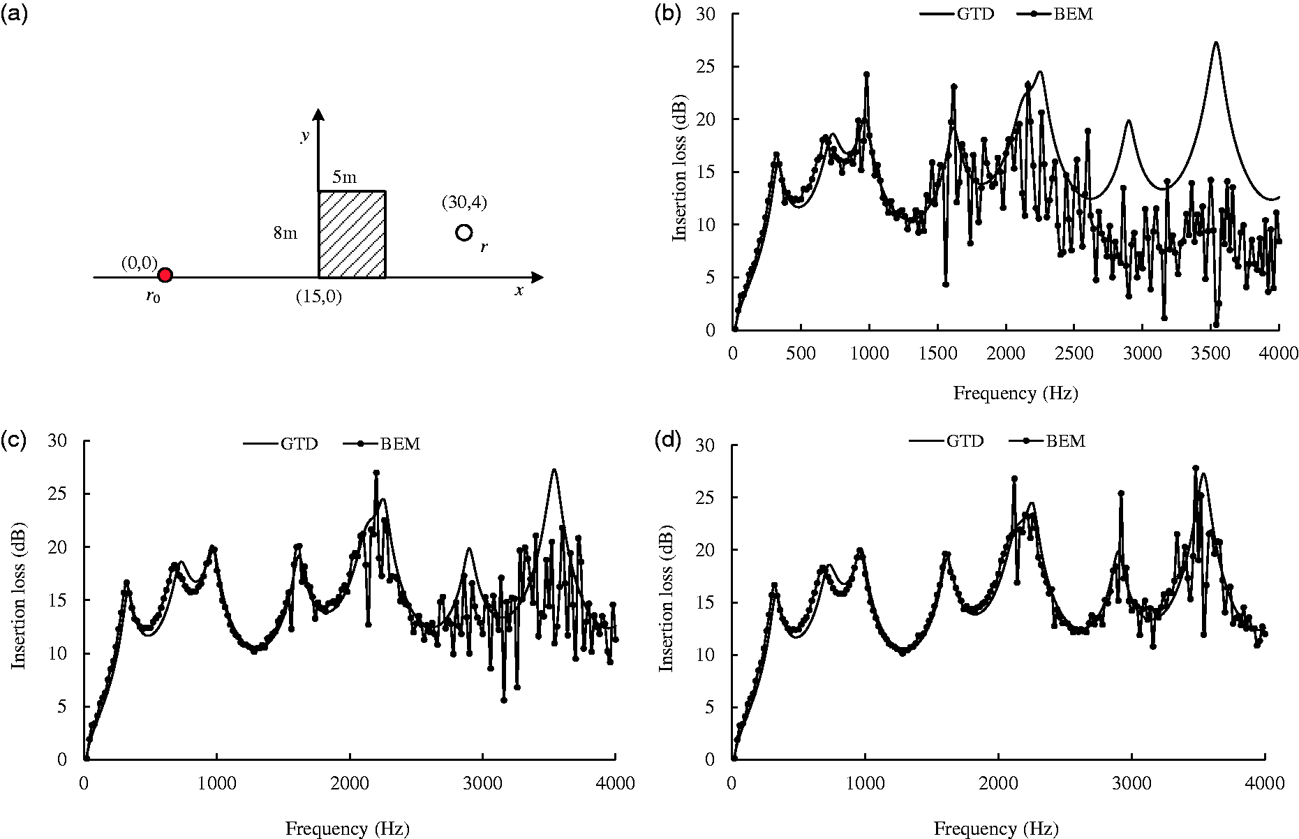

Impact of the element length on the results

GTD is a method that calculates noise levels of receivers by finding the theoretical solutions of acoustic wave equations. For a complex scene such as balconies building region, GTD is out of operation as the theoretical solutions are inexistent. Thus, BEM are used to get the numerical solutions of acoustic wave equations. As the accuracy of GTD has been verified by scholars,³⁸ comparisons to BEM with various factors were helpful for accuracy analysis of BEM.

As shown in Figure 2, calculations were performed with sound wave frequencies in the range of 20–4000 Hz.

When the frequency is below 1500 Hz, the BEM yields results consistent with those of the GTD if the element length l is λ. A difference (approximately 5 dB), which appears when the frequency exceeds 2000 Hz, increases (10–20 dB) for frequencies greater than 3000 Hz. The coincidence degree of the curves increases significantly if the length of each element is subdivided into λ/2. However, a comparatively large deviation (over 10 dB) still occurs when the frequency exceeds 3300 Hz. If the length of each element is further subdivided into λ/5, then the BEM results are consistent with the GTD results at a frequency below 4000 Hz. Thus, the accuracy of the BEM results is found to be strongly correlated to the element length. A λ/5 elements length is adopted in the behind dissertation.

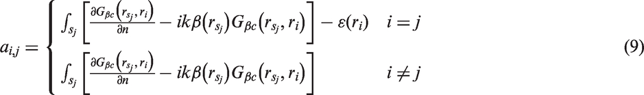
Due to BEM discretization of the boundary integral equations, the method is actually a type of mathematical approximation to the original physical problem. In terms of calculation accuracy, the number of parts into which an element is subdivided directly correlates to the accuracy of the computed solution. Each element in the coefficient matrix [A] is actually an approximate value that is determined by the discretization of the boundary and is independent of the calculation precision. The density of the coefficient matrix [A] is directly proportional to the results influence caused by these approximate values have on the results. If the results deviate greatly from actual conditions, then further subdivision of the elements is required to improve the accuracy of the approximation.

Impact of the element length on the efficiency

The element length determines the number of elements, and the computed time includes the expense of equation establishment and the generation of the solution. After getting the computation times of different element length, curve fitting with a principle of least squares was used while describing the relationship between the element length and efficiency. Figure 3 shows the relationship between the calculation efficiency and the element length for an 800 Hz sound. The computed time increases exponentially with the subdivision precision of the element. The relationship of time (z) and element length (x) can be described as a matched curve: z = 4284.3e^−13.92x.

Figure 3.

The relationship between the element length and the efficiency.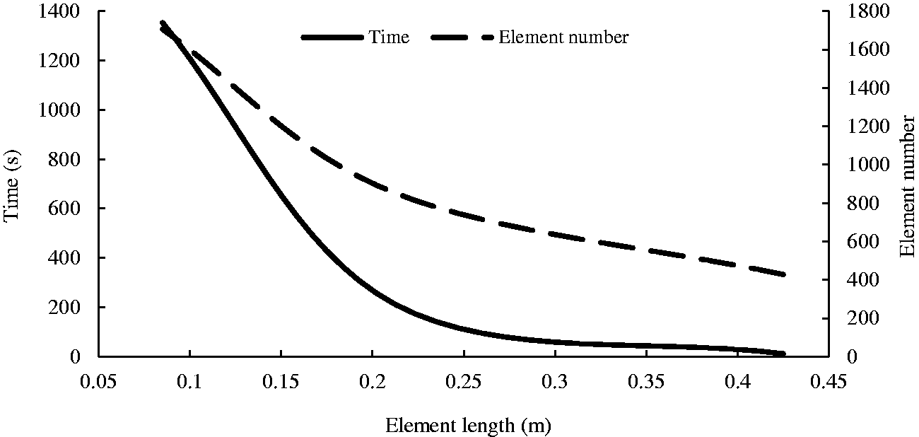

The impacts of the accuracy of Hankel functions on the results

The precision of the final result may be affected by the Hankel functions’ calculation accuracy (in equations (5) and (13)). The impacts of Hankel functions were analyzed as follows.

Hankel functions are given by

H_{α}^{1} = J_{α} (x) + {iY}_{α} (x)

(14)

H_{α}^{2} = J_{α} (x) - {iY}_{α} (x)

(15)

When x is comparatively small

J_{α} (x) = \sum_{k = 0}^{\infty} (- 1)^{k} \frac{(\frac{1}{2} x)^{α + 2 k}}{k! (α + k)!}

(16)

Y_{α} (x) = \frac{1}{π} {- \sum_{k = 0}^{α - 1} \frac{(α - k - 1)!}{k!} (\frac{1}{2} x)^{- α + 2 k} + \sum_{k = 0}^{\infty} (- 1)^{k} \frac{(\frac{1}{2} x)^{α + 2 k}}{k! (α + k)!} [2 \ln (\frac{1}{2} x) - ψ (k + 1) - ψ (α + k + 1)]}

(17)

where

ψ (k + 1) = - γ + 1 + \frac{1}{2} + \frac{1}{3} + \dots + \frac{1}{k}

, Euler’s constant

γ = 0.5772156649 \dots

. When x is large enough, equations (16) and (17) converge quite slowly, and the following asymptotic formula is applicable for calculation

J_{α} (x) = \sqrt{\frac{2}{π x}} [P_{α} (x) cos (x - \frac{π}{2} (α + \frac{1}{2})) - Q_{α} (x) sin (x - \frac{π}{2} (α + \frac{1}{2}))]

(18)

Y_{α} (x) = \sqrt{\frac{2}{π x}} [Q_{α} (x) cos (x - \frac{π}{2} (α + \frac{1}{2})) + P_{α} (x) sin (x - \frac{π}{2} (α + \frac{1}{2}))]

(19)

here

P_{α} (x) = 1 - \frac{(4 α^{2} - 1^{2}) (4 α^{2} - 3^{2})}{2! (8 x)^{2}} + \frac{(4 α^{2} - 1^{2}) (4 α^{2} - 3^{2}) (4 α^{2} - 5^{2}) (4 α^{2} - 7^{2})}{4! (8 x)^{4}} - \dots

(20)

Q_{α} (x) = \frac{(4 α^{2} - 1^{2})}{8 x} - \frac{(4 α^{2} - 1^{2}) (4 α^{2} - 3^{2}) (4 α^{2} - 5^{2})}{3! (8 x)^{3}} + \dots

(21)

In this dissertation, the first m terms of equations (16), (17), (20), and (21) were taken to calculate Hankel functions. Equations (16) and (17) are adopted if x < m/2, whereas equations (18) to (21) are applicable if x ≥ m/2. The problem of sound diffraction in Figure 2(a) has been taken as an example, so as to study how the final results of insertion loss ΔL are affected by the calculation accuracy of Hankel functions. The acoustic admittance β = (0, 0), the sound source frequency is 800 Hz. The computed results of ΔL have been listed in Figure 4 when m = 4, 6 … 30. Obviously, the results are insignificantly affected by the calculation accuracy of Hankel functions. During calculation, the results of ΔL are accurate to eight digits as long as the term number of the progression exceeds 22.

Figure 4.

The relationship between the term numbers of the progression and the ΔL results.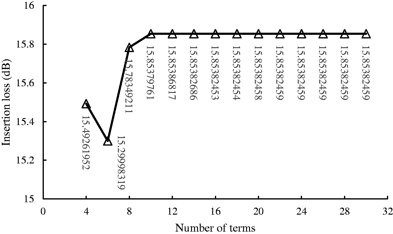

The impacts of the accuracy of numerical integration on the results

During the establishment of linear equations (7), all elements in matrix [A] were obtained through integration of equation (9) with numerical integration approaches. The precision of all elements in matrix [A] is directly influenced by the integration accuracy, which further affects the final results.

Two numerical integration methods, midpoint rectangle rule and composite four-point Gaussian quadrature rule, have been compared in this dissertation. Under the midpoint rectangular rule, an integrating interval is equally divided into k subintervals, and the function value at the midpoint of a subinterval is taken as the value of the subinterval (totally k computing points are taken). Whereas under the composite four-point Gaussian quadrature rule, the integrating interval is also equally divided into k subintervals, and four computing points are taken within each subinterval in a certain proportion and weighting (4k computing points are taken in all). Likewise, Figure 2(a) has been taken for example. The first 26 terms of the progression in the Hankel function were selected during calculation. The midpoint rectangle rule and the composite four-point Gaussian rule were, respectively, used in integration, and other conditions were the same as those in the previous example. The relationship between the number of computing points (taken during the integration of each element) and the final results of ΔL has been presented in Figure 5. It is clear that the number of integration points has relatively little effect on the results, and the composite four-point Gaussian rule has a higher convergence rate than the midpoint rectangle rule. During calculation with the four-point Gaussian rule, an accuracy of eight digits could be reached as long as more than 20 computing points are taken in each element.

Figure 5.

The relationship between the number of computing points and the results of ΔL.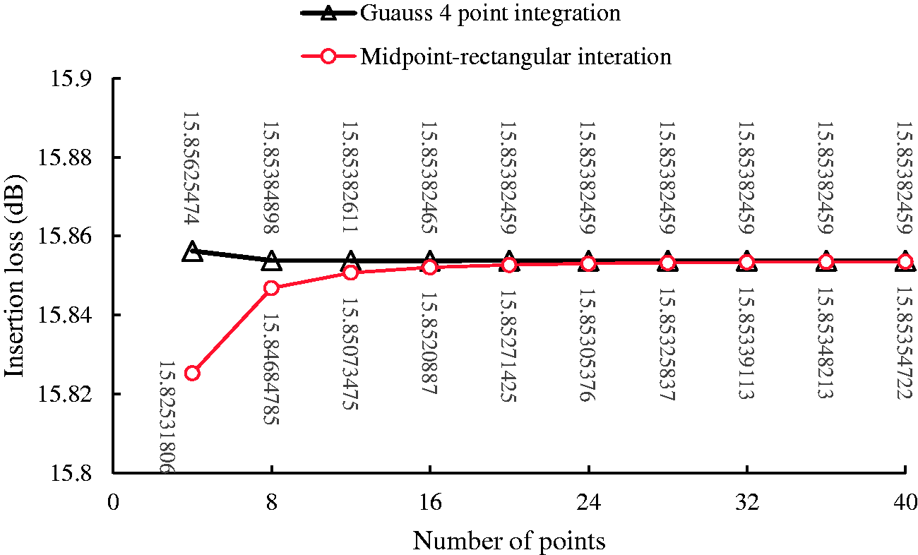

Sound calculations of buildings with different aspect ratios

Scene description

In actual scenarios, the buildings near roadways vary in size, and the aspect ratios of these buildings may have an effect on sound attenuation. The 2D building depicted in Figure 6(a) was used as an example to study the effect of the aspect ratio on sound propagation. The sound frequency is set to 800 Hz. The widths of the building are set to 3, 5, 8, 10, and 15 m, corresponding to aspect ratios r of 0.15, 0.25, 0.4, 0.5, and 0.75, respectively.

Figure 6.

The relationship between the aspect ratio and the ΔL efficiency (horizontal). (a) Depiction of chosen plane (in m) and (b) results of insertion losses.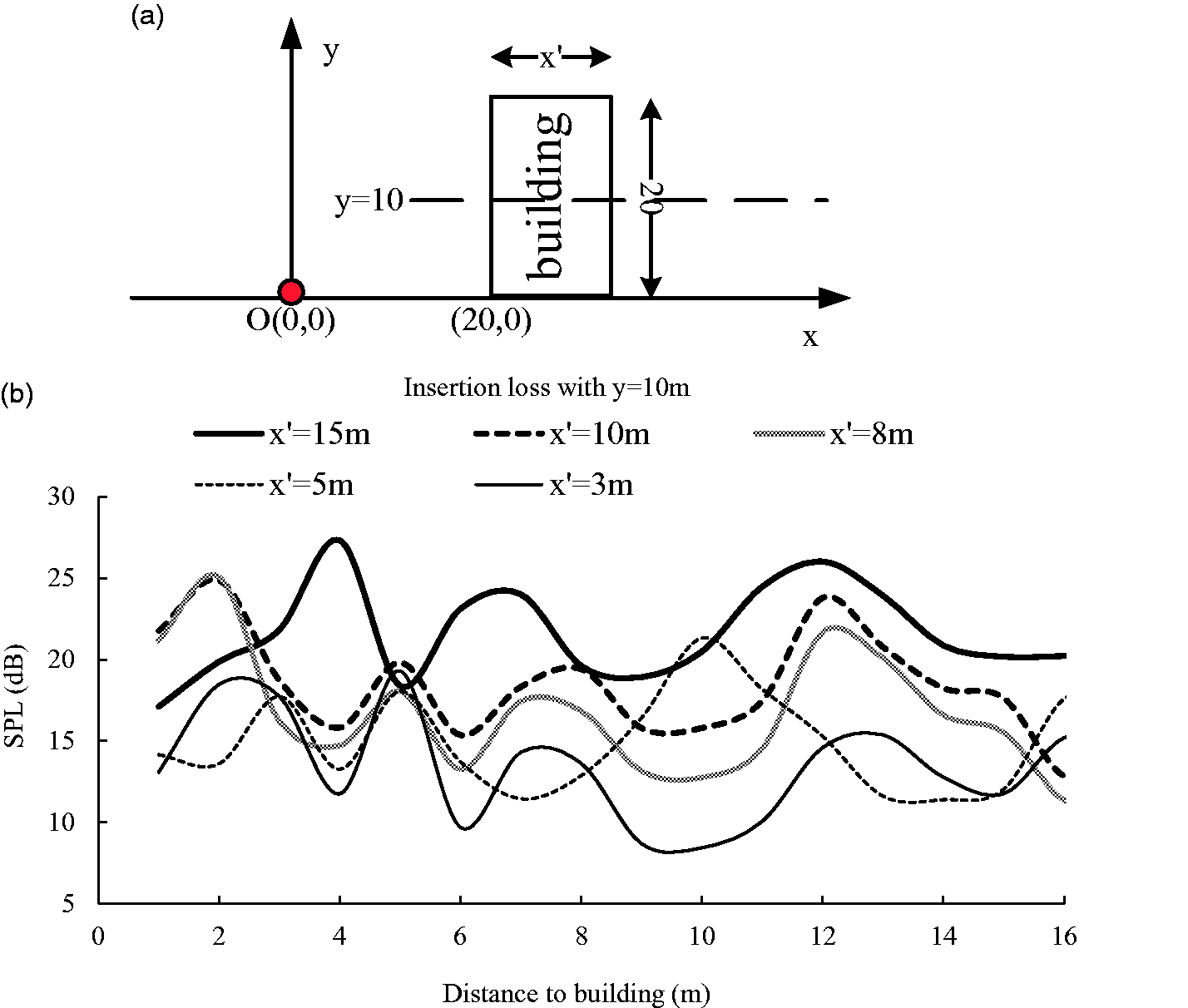

Sound propagation properties for different aspect ratios

The plane y = 10 is chosen to study the properties of the horizontal changes of the insertion loss using different aspect ratios. The relationship between the distance x′ (distance of the receiver to the building) and the result of ΔL is presented in Figure 6(b). For different aspect ratios, it is clear that ΔL remains within a range around a fixed value with a limited x′, and that the average ΔL increases with r. For r values of 0.15, 0.25, 0.4, 0.5, and 0.75, the corresponding fixed ΔL value is 13.62, 15.23, 16.20, 18.01, and 21.53 dB, respectively.

The plane x = 40 is chosen to study the properties of the vertical changes of the insertion loss using different aspect ratios, as described in Figure 7(a). Figure 7(b) illustrates the relationship between the heights of the receivers and ΔL of the buildings. The figure indicates the following: the insertion loss ΔL presents a trend of fluctuating decay at increasing heights, and, similar to the performance at the horizontal plane, ΔL increases as r grows; when the height is less than 10 m, the insertion loss remains within a fixed value range, with values of 14.82, 27.29, 31.27, 34.31, and 36.73 dB for five different values of r (0.15, 0.25, 0.4, 0.5, and 0.75, respectively); a decrease in ΔL occurs when the height exceeds the height of the building (20 m), and ΔL approaches zero as the height is further increased beyond the source visibility height (40 m).

Figure 7.

The relationship between aspect ratio and the ΔL efficiency (vertical). (a) Depiction of chosen plane (in m) and (b) results of insertion losses.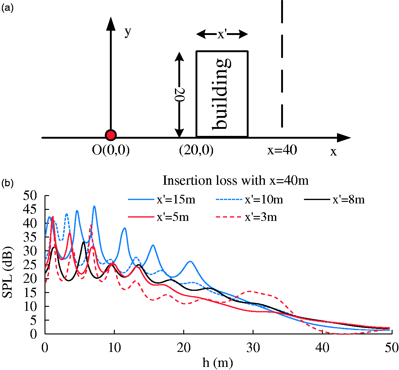

Study of a balconied building near a roadway using BEM

Sound field of the building region

Balconies are common components of a building’s façade. A sound propagation study of the building region is especially significant in the region of balconies, whose acoustic environment can have a large effect on people inside the building. An example is modeled and has the configuration described in Figure 8. The thickness of the balcony walls and floor construction is 0.1 m. The sound frequency is set to 800 Hz. The model is simplified from a 3D model, in which the source is an infinite coherent line source parallel to the outer façade of the building.

Figure 8.

Sketch of the balconied building and the roadway (in m). (a) Sketch map and (b) depiction of chosen planes and points.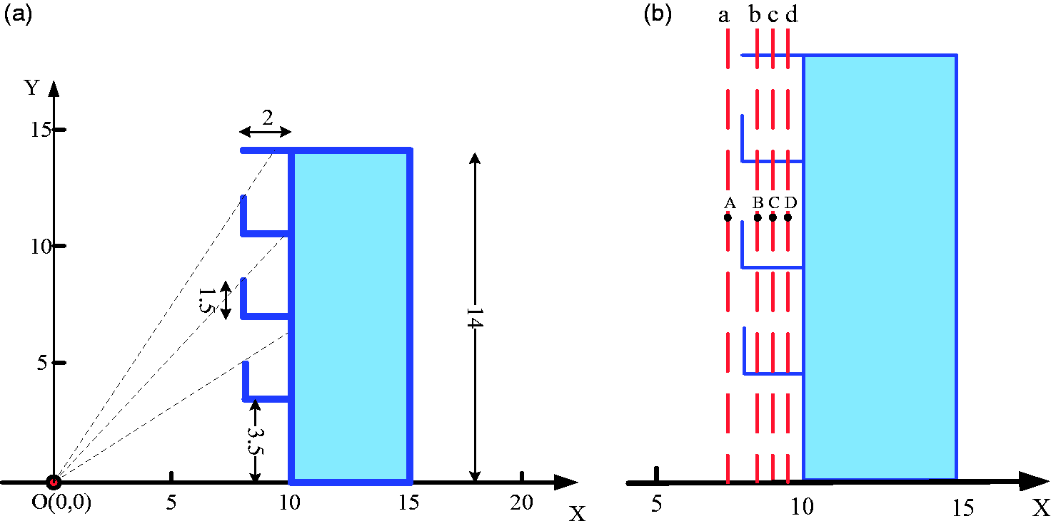

A grid of 100 × 100 mesh points is set in the region. For each point, the SPL is calculated via BEM; the calculated sound field of this region is depicted in Figure 9(a). The level difference is defined as LD = SPLa − SPLb, where SPLa is the SPL at the receiver when the building is absent, and SPLb is the SPL at the same receiver when the building is present. The value of LD can describe the insertion loss of barriers (building and balconies) behind them and the SPL changes in front of the buildings. Figure 9(b) shows the LD before and after the building is present. The building and balconies have an obvious shading effect on the propagating sound, and the maximum LD is greater than 15 dB.

Figure 9.

Sound field and LD of the balconied building (in dB). (a) Sound field of the building region and (b) lever difference of the building region. LD: level difference.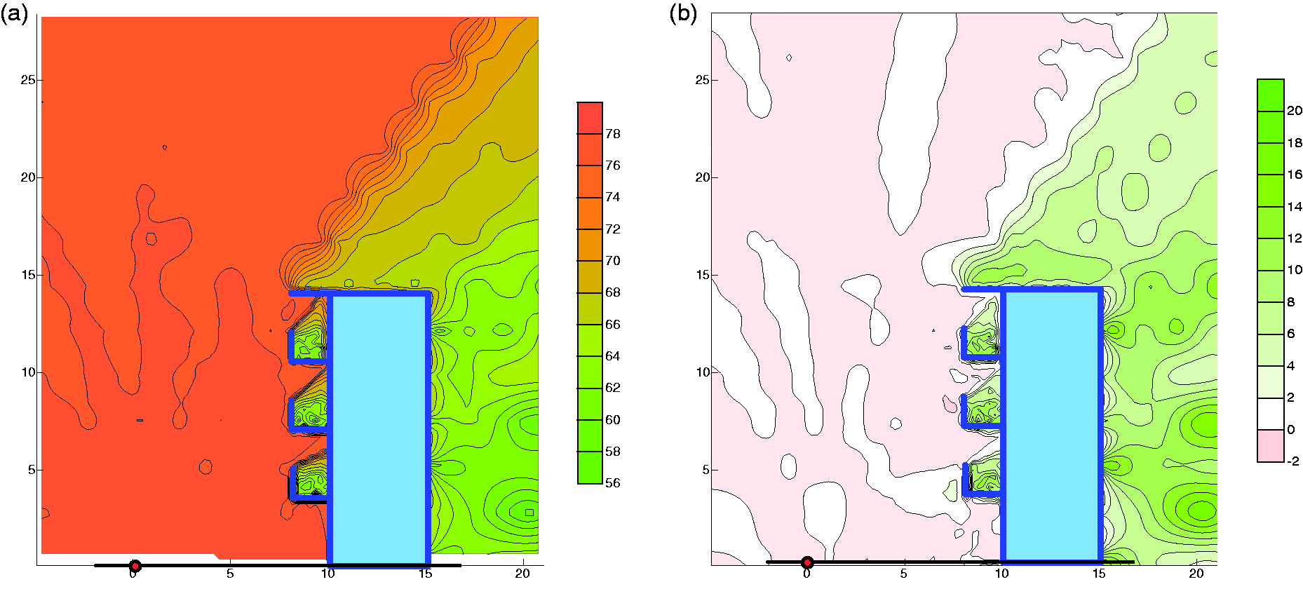

Sound attenuation on different floors

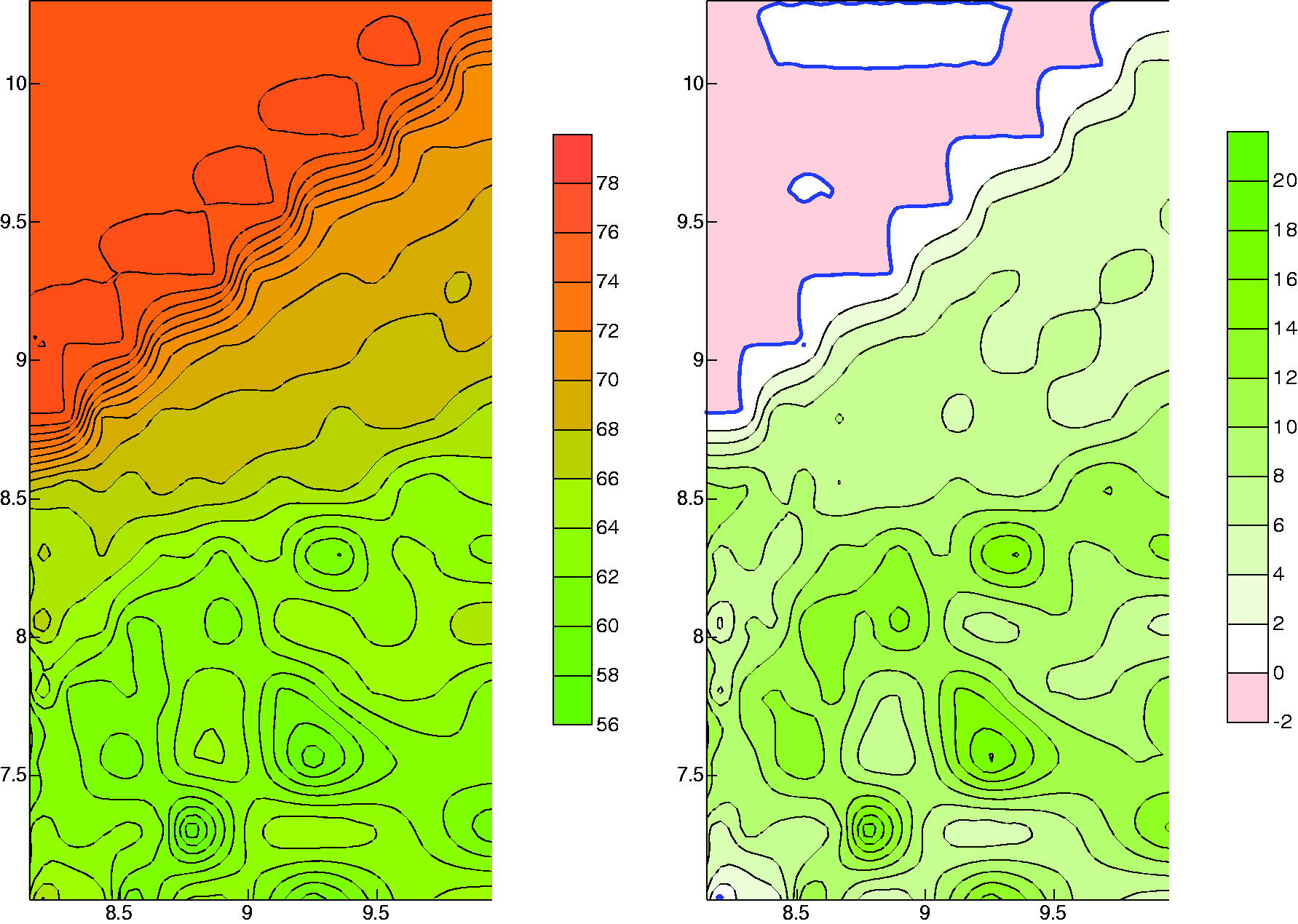
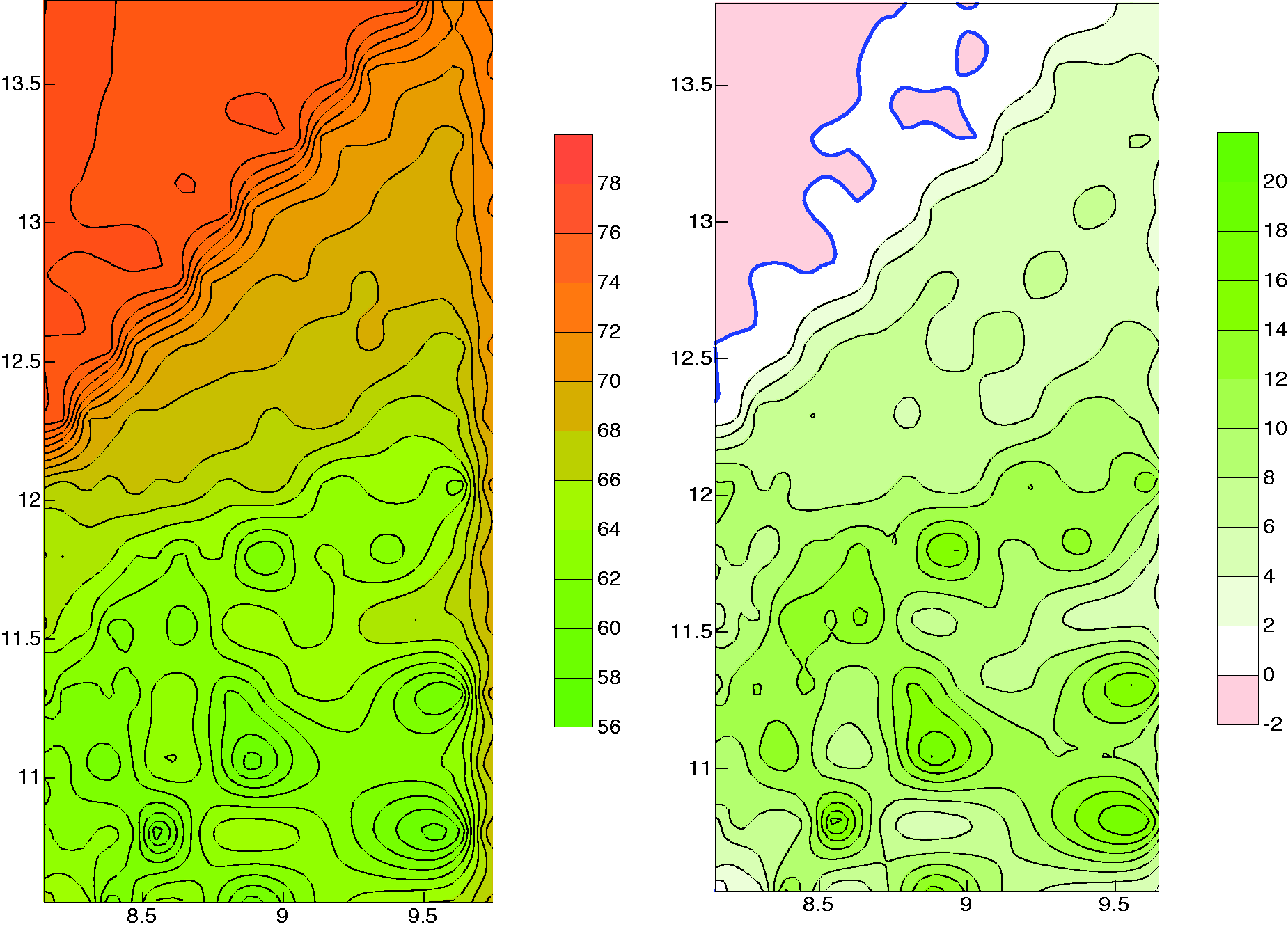
The sound attenuation on different floors with balconies is considered in this section. The micromesh sound field and the LD of different floors are depicted in Figures 10 to 12. There is an obvious line (LD = 0 dB) at each floor, which means the boundary of the balconies’ shadow areas. Though values of the SPL and LD share the approximately same ranges with 56–80 and −2 to 20 dB, respectively, different floors present diverse sound fields due to the various geometrical conditions. Additionally, due to the differences of the relative locations between the source and the balconies, the shadow zone region is greater on higher floors and the distributions of noise are more tanglesome. In addition, at the top of the shadow zone, the insertion loss is not as distinct as it is at other areas because of the reflections from the ceilings.

Figure 10.

Sound field and LD of the second floor (in dB). LD: level difference.

Figure 11.

Sound field and LD of the third floor (in dB). LD: level difference.

Figure 12.

Sound field and LD of the fourth floor (in dB). LD: level difference.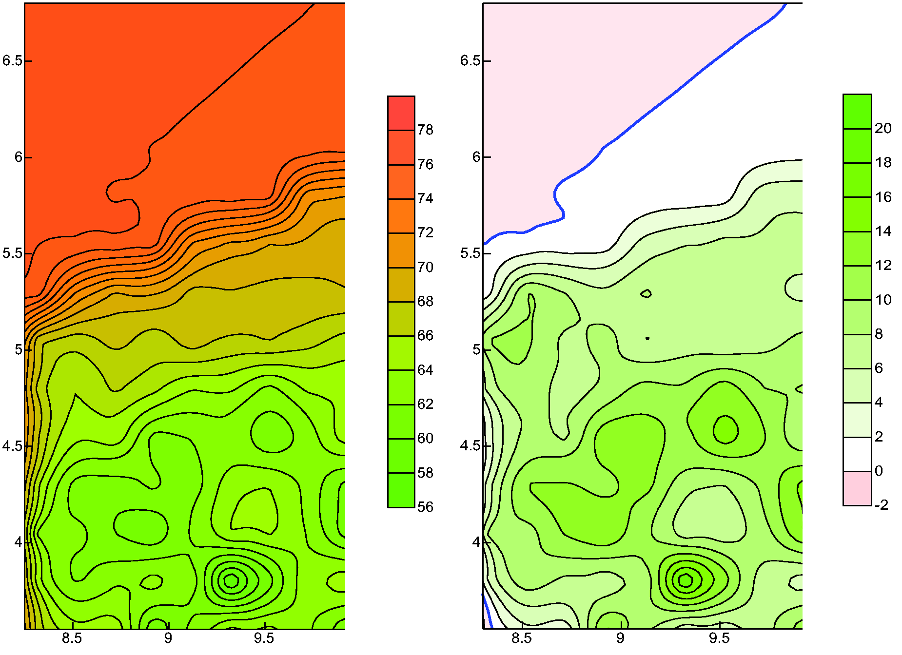

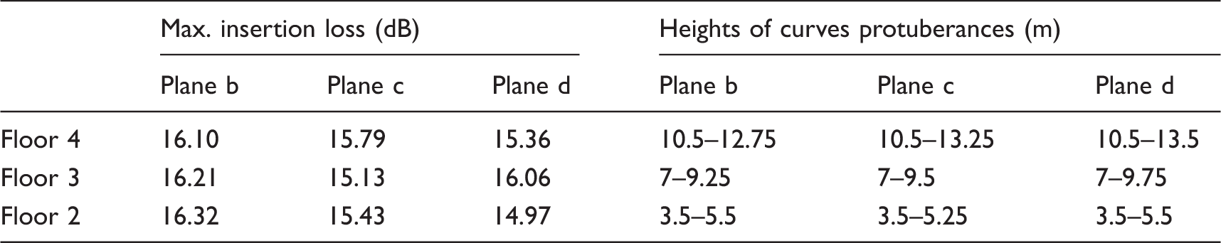
To discover the sound attenuation effects on different floors, planes a, b, c, and d are chosen for noise calculation analyses. As indicated by the lines in Figure 8(b), plane a is 0.5 m from the outer façade, and lines b, c, and d are 0.5, 1.0, and 1.5 m, respectively, from the rear wall of balconies. SPL and LD of the four planes are calculated, as depicted in Figure 13.

Figure 13.

SPL and LD of different floors. (a) Sound pressure level and (b) level different. LD: level difference; SPL: sound pressure level.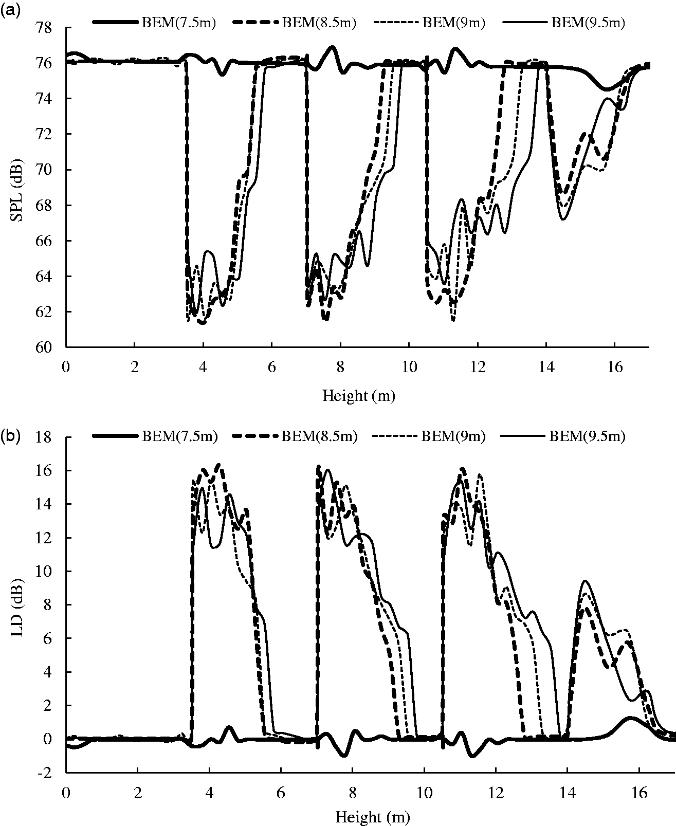

In Figure 13, it is clear that balconies have obvious sound-shading effects, and that a trend of decline of SPL with height is observed. For plane a, which is outside of the outer façade of the balconies, LD varies between −1.87 and 0.59 dB. Due to the effect of the balconies, the SPL and LD curves of plane a fluctuate more than at heights of 3.5–5, 7–8.5, and 0.5–12 m (the heights of the balconies). Large sound attenuation occurs when planes b, c, and d pass through the balconies. The maximum LD values and the ranges of the protuberances of the curves are listed in Table 1. It can be seen that there is almost no difference in maximum LD between the different floors as all the values are approximately 15 dB. The height ranges of plane b where large attenuations appear become larger when the plane moves to c and d. The ranges of the protuberances of the curves reveal the scope of the balconies’ influence, with the shadow area being greater at the room side.

Table 1.

Sound attenuation levels of the balcony areas and the shadow areas.

	Max. insertion loss (dB)			Heights of curves protuberances (m)
	Plane b	Plane c	Plane d	Plane b	Plane c	Plane d
Floor 4	16.10	15.79	15.36	10.5–12.75	10.5–13.25	10.5–13.5
Floor 3	16.21	15.13	16.06	7–9.25	7–9.5	7–9.75
Floor 2	16.32	15.43	14.97	3.5–5.5	3.5–5.25	3.5–5.5

The sound attenuation levels of the balcony areas and shadow areas on different floors are listed in Table 2. Combined with the sound fields shown in Figures 10 to 12, the maximum insertion losses of balconies appear at the bottom of the balcony areas. The values of the maximum insertion losses at the second, third, and fourth floors are 16.78, 16.45, and 16.32 dB, respectively, and appear at the coordinate points (3.75, 9.3), (7.25, 8.75), and (10.75, 8.6), respectively. Considering all of the values and shadow areas, the balconies on the higher floors result in better sound abatement.

Table 2.

Sound attenuation levels of the balcony areas and the shadow areas (in dB).

SPL	Max. insertion loss	Min. value	Average value
SPL	Max. insertion loss	Min. value	Balcony area	Shadow area
Floor 4	16.32	54.22	60.24	60.51
Floor 3	16.45	54.34	62.88	59.36
Floor 2	16.78	53.42	64.32	60.21
Floor 1	–	75.98	76.04	–

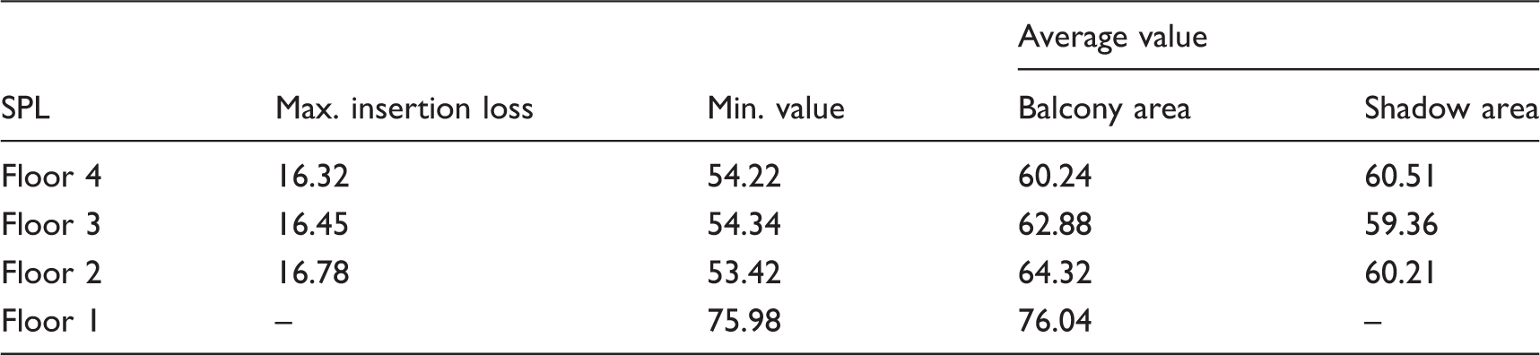
SPL: sound pressure level.

Impacts of different frequencies on the sound attenuation of balconies

As there is a wide range of sound frequencies, the shading effects of balconies under differing frequencies are different. Thus, study of the propagation of sound in the balcony areas for different frequencies is required, especially in the range of the typical low and medium frequencies of road traffic noise.

As depicted in Figure 8(b), points A, B, C, and D located at planes a, b, c, and d, respectively, are chosen to calculate the LD with sound wave frequencies in the range of 20–4000 Hz. The height of the chosen points is 8.5 m, and the results are shown in Figure 14. For point A, which is outside of the balcony, the LD is in a range around approximately 0.5 dB with different frequencies. Thus, the LD results are apparently not related to the frequency, as there is only direct and reflected sound at point A. However, the LD presents a distinct pattern regarding points B, C, and D. The LD, which is only approximately 3 dB when the sound wave frequency is below 500 Hz, increases with the frequency. When the wave frequency reaches 4000 Hz, the LDs of B, C, and D are approximately 14, 13, and 10 dB, respectively. Thus, we can conclude that the LD of the balconies is significantly related to the sound wave frequency, with the balconies having a greater shading effect on higher frequency sound.

Figure 14.

The relationship between frequency and the level difference. (a) Level difference of point A, (b) level difference of point B, (c) level difference of point C, and (d) level difference of point D.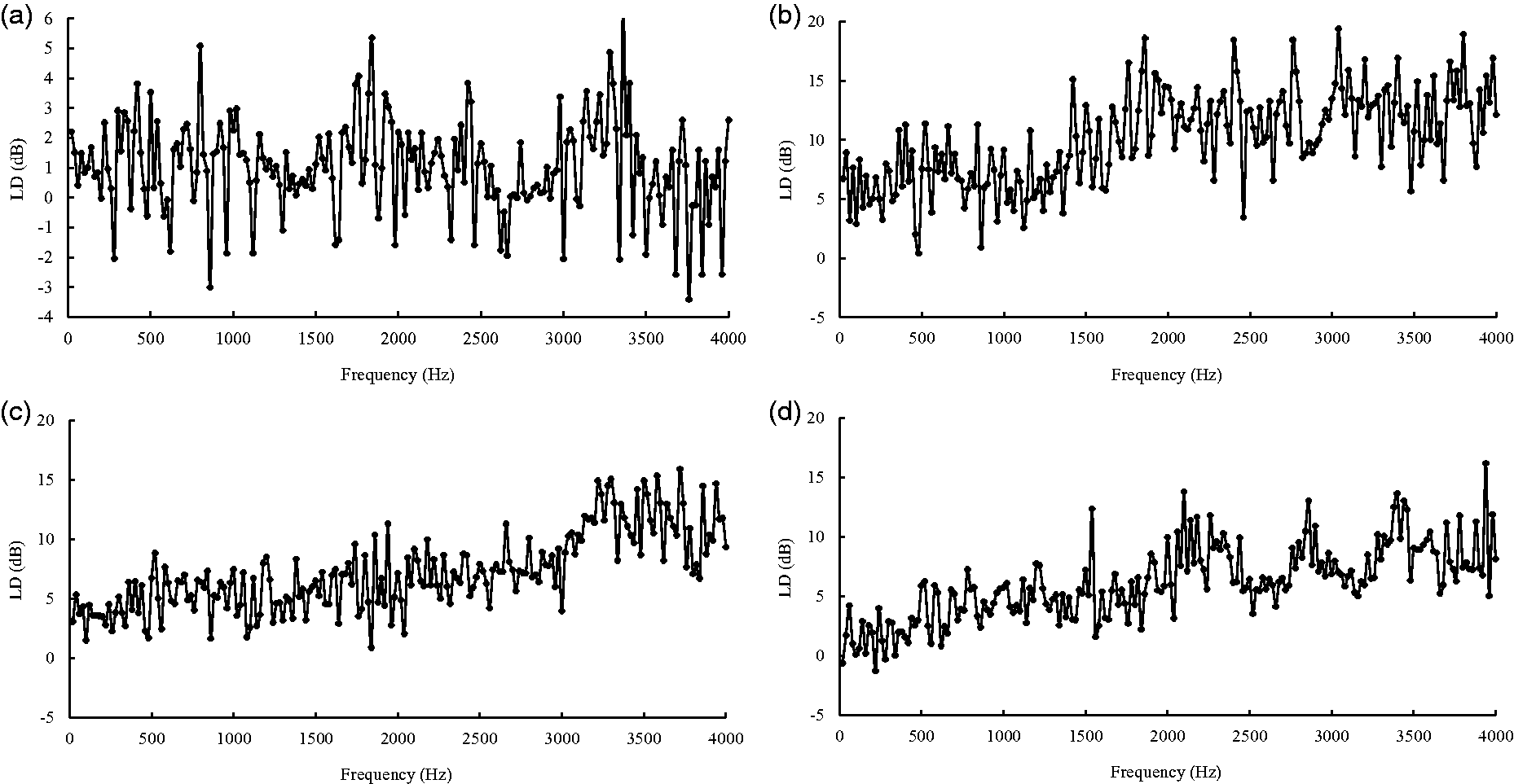

The frequency of road traffic noise varies from 40 to 4000 Hz. Because of the diversity of physical structures, different types of vehicles have different sound emissions,³⁹ and, when vehicles travel at a normal speed, the frequencies of light, medium, and heavy vehicles concentrate at 800, 630, and 500 Hz of the 1/3-octave spectrum, respectively.

The results of the LD under the three frequencies mentioned above are depicted in Figure 15. The average insertion losses of the second to fourth floors are approximately 15 dB when the frequency is 800 Hz, 13 dB when the frequency is 630 Hz, and 9 dB when the frequency is 500 Hz. The attenuation is more obvious for noise from light vehicles compared with noise from medium and heavy vehicles, with D values of 2 and 6 dB, respectively. The shadow area could be ranked as follows: 500 Hz < 630 Hz < 800 Hz; this relationship indicates that the lower frequency sound can bypass the barrier more easily. Thus, flow control of heavy vehicles whose sound is concentrated in low frequencies is an effective measure to improve the acoustic environment near roadways.

Figure 15.

The level difference (LD) for three typical frequencies.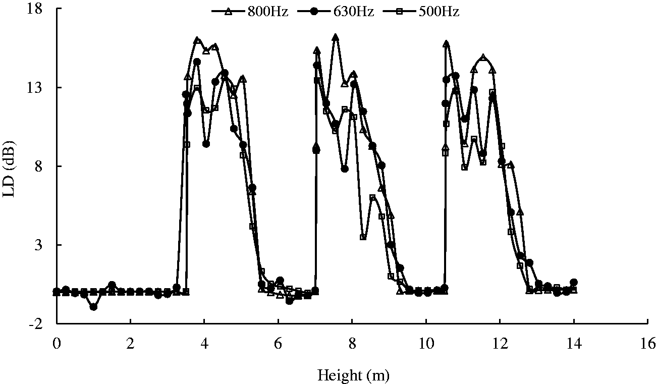

Conclusion

BEM was used to calculate the sound field of a building region produced by a nearby stream of road traffic. Noise distribution of balconies building area instead of only typical points was depicted, and the noise analysis based on this is not only global but also local.

The computed results are softly affected by the calculation accuracy or the numerical integration accuracy of Hankel functions. However, the element division has relatively significant effects on such results. The computed time increases exponentially with the reciprocal of the length scale of the elements.

The insertion loss ΔL increases with the aspect ratio r. ΔL is in a range around a fixed value, with a limited x′ in the horizontal plane. While the properties are different for a vertical plane: when the height is low enough, the insertion loss is in a range around a fixed value, and a decay, which appears when the height reaches the building’s height, approaches zero as the height increase to the source visible height.

The results of the LD on different floors demonstrate that the scope of influence of the balconies is greater on the room side. The maximum insertion losses of the chosen lines inside the balconies are all approximately 15 dB at different floors, while the LD outside of the balconies varies from −1.87 to 0.59 dB.

Higher sound frequencies are correlated to larger insertion loss, and for the points from the rear wall of the balcony, the insertion loss is increasing from 3 dB to > 10 dB as the frequency increases from 20 to 4000 Hz. Attenuation is more prominent for noise from light vehicles compared with noise from medium and heavy vehicles, where a D value of 2 and 6 dB is found, respectively. As a result, flow control of heavy vehicles can be used as a considerable measure to abate road traffic noise.

Footnotes

Declaration of conflicting interests

The author(s) declared no potential conflicts of interest with respect to the research, authorship, and/or publication of this article.

Funding

The author(s) disclosed receipt of the following financial support for the research, authorship, and/or publication of this article: This work is supported by the National Natural Science Foundation of China (No. 11574407), the Fundamental Research Funds for the Central Universities (No. 17lgpy55), and the Foundation for Distinguished Young Talents in Higher Education of Guangdong, China (No. 2016KQNCX093).

References

Monazzam

Abolhasannejad

BNM

, et al. Noise pollution in old and new urban fabric with focus on traffic flow. J Low Freq Noise V A 2016; 35: 257–263.

Mihajlov

Prascevic

. Permanent and semi-permanent road traffic noise monitoring in the City of Nis (Serbia). J Low Freq Noise V A 2015; 34: 251–268.

Remillieux

Corcoran

Haac

, et al. Experimental and numerical study on the propagation of impulsive sound around buildings. Appl Acoust 2012; 73: 1029–1044.

Morillas

JMB

Gonzalez

Gozalo

. A review of the measurement procedure of the ISO 1996 standard. Relationship with the European noise directive. Sci Total Environ 2016; 565: 595–606.

Lopez

. Objective evaluation of a simulation of the acoustics of a medieval urban space used for dramatic performances. Appl Acoust 2015; 88: 38–43.

Yousefzadeh

Hodgson

. Energy- and wave-based beam-tracing prediction of room-acoustical parameters using different boundary conditions. J Acoust Soc Am 2012; 132: 1450–1461.

Takekawa

Mikada

Imamura

. A mesh-free method with arbitrary-order accuracy for acoustic wave propagation. Comput Geosci 2015; 78: 15–25.

Yao

Zhou

. Numerical treatment of 2D acoustic problems with the cell-based smoothed radial point interpolation method. Appl Acoust 2012; 73: 557–574.

Yang

Guo

. Computation of acoustic transfer matrices of swirl burner with finite element and acoustic network method. J Low Freq Noise V A 2015; 34: 169–184.

10.

Kim

Kang

, et al. Sound diffraction by multiple wedges and thin screens. Appl Acoust 2005; 66: 1102–1119.

11.

, et al. A successive three-point perturbation method for fast ray tracing in complex 2D and 3D geological models. Tectonophysics 2014; 627: 72–81.

12.

Chen

Cai

, et al. Dynamic simulation of traffic noise by applying ray tracing method based on indoor space partitioning. Acta Acust United Ac 2014; 100: 467–476.

13.

Markovic

Antonacci

Sarti

, et al. 3D beam tracing based on visibility lookup for interactive acoustic modeling. IEEE Trans Vis Comput Graph 2016; 22: 2262–2274.

14.

Wilson

Hopkins

. Analysis of bending wave transmission using beam tracing with advanced statistical energy analysis for periodic box-like structures affected by spatial filtering. J Sound Vib 2015; 343: 138–161.

15.

Wilson

Hopkins

. Analysis of bending wave transmission using beam tracing with advanced statistical energy analysis for periodic box-like structures affected by spatial filtering. J Sound Vib 2015; 341: 138–161.

16.

Viveiros

Gibbs

. An image model for predicting the field performance of acoustic louvers from impulse measurements. Appl Acoust 2003; 64: 713–730.

17.

Funkhouser

Tsingos

Carlborn

, et al. A beam tracing method for interactive architectural acoustics. J Acoust Soc Am 2004; 107: 1405–1412.

18.

De Coensel

De Muer

Yperman

, et al. The influence of traffic flow dynamics on urban soundscapes. Appl Acoust 2005; 66: 175–194.

19.

Hornikx

Forssen

. The 2.5-dimensional equivalent sources method for directly exposed and shielded urban canyons. J Acoust Soc Am 2007; 122: 2532–2541.

20.

Yang

Shield

. Development of a ray tracing computer model for the prediction of the sound field in long enclosures. J Sound Vib 2000; 229: 133–146.

21.

Dehghan

Shirzadi

. The modified dual reciprocity boundary elements method and its application for solving stochastic partial differential equations. Eng Anal Bound Elem 2015; 58: 99–111.

22.

Peplow

. On the efficiency of screens near roadside cuttings. J Sound Vib 2006; 298: 982–1000.

23.

Liu

, et al. A coupled ES-BEM and FM-BEM for structural acoustic problems. Noise Control Eng J 2014; 62: 196–209.

24.

Chen

. Adaptive integration method based on sub-division technique for nearly singular integrals in near-field acoustics boundary element analysis. J Low Freq Noise V A 2014; 33: 27–45.

25.

Ning

. Numerical simulation of finite amplitude standing waves in acoustic resonators using finite volume method. Wave Motion 2013; 50: 135–145.

26.

Liu

, et al. Numerical investigation of ES-FEM with various mass redistribution for acoustic problems. Appl Acoust 2015; 89: 222–233.

27.

Georgiev

Krylov

Winward

RETB

. Simplified modelling of vehicle interior noise: comparison of analytical, numerical and experimental approaches. J Low Freq Noise V A 2006; 25: 69–92.

28.

. Numerical analysis and active control simulation of sound transmission from air to water through plates. J Low Freq Noise V A 2011; 30: 149–160.

29.

Hiraishi

Tsutahara

Leung

RCK

. Numerical simulation of sound generation in a mixing layer by the finite difference lattice Boltzmann method. Comput Math Appl 2010; 59: 2403–2410.

30.

Tsutahara

Kataoka

Shikata

, et al. New model and scheme for compressible fluids of the finite difference lattice Boltzmann method and direct simulations of aerodynamic sound. Comput Fluids 2008; 37: 79–89.

31.

Chen

, et al. Radial integration boundary element method for acoustic eigenvalue problems. Eng Anal Bound Elem 2013; 37: 1043–1051.

32.

Ishizuka

Fujiwara

. Performance of noise barriers with various edge shapes and acoustical conditions. Appl Acoust 2004; 65: 125–141.

33.

Hothersall

Horoshenkov

Mercy

. Numerical modeling of the sound field near a tall building with balconies near a road. J Sound Vib 1996; 198: 507–515.

34.

Padron

Aznarez

Maeso

. 3-D boundary element-finite element method for the dynamic analysis of piled buildings. Eng Anal Bound Elem 2011; 35: 465–477.

35.

Marburg

Schneider

. Influence of element types on numeric error for acoustic boundary elements. J Comput Acoust 2003; 11: 363–386.

36.

Marburg

. Numerical damping in the acoustic boundary element method. Acta Acust United Ac 2016; 102: 415–418.

37.

Nolte

Marburg

. Preface – wave based numerical methods. J Comput Acoust 2007; 15: 7–8.

38.

Shen

. Hankbook of acoustics, Beijing: Sci Press, 2004.

39.

Ascari

Licitra

Teti

, et al. Low frequency noise impact from road traffic according to different noise prediction methods. Sci Total Environ 2015; 505: 658–669.

Sound field study of a building near a roadway via the boundary element method

Abstract

Keywords

Introduction

BEM equations for sound fields

Establishment of the boundary integral equation

BEM used to solve boundary integral equations

A factor analysis of the computed results

Impact of the element length

Impact of the element length on the results

Impact of the element length on the efficiency

The impacts of the accuracy of Hankel functions on the results

The impacts of the accuracy of numerical integration on the results

Sound calculations of buildings with different aspect ratios

Scene description

Sound propagation properties for different aspect ratios

Study of a balconied building near a roadway using BEM

Sound field of the building region

Sound attenuation on different floors

Impacts of different frequencies on the sound attenuation of balconies

Conclusion

Footnotes

Declaration of conflicting interests

Funding

References