Sage Journals: Discover world-class research

Abstract

There is general agreement that a firm’s scarce marketing resources should be managed for the purpose of long-term profitable growth. Putting that premise into practice is difficult, as only the short-term impact of marketing actions can be readily observed. Persistence modeling has become a well-accepted tool for long-run impact detection. Its consistent use across a broad range of settings has resulted in novel empirical generalizations on the long-run effectiveness of several marketing instruments and has contributed unique insights on, among others, (i) the marketing-finance interface, (ii) the role of new media, and (iii) the mediating role of a broad set of mindset metrics. Moreover, the recent addition of a more normative focus has added considerably to the actionability of these insights.

Keywords

marketing mix time series models

Time series data and time series models

Marketing data are often ordered, at evenly spaced intervals, over time. Examples include behavioral (e.g. the number of web clicks or new Facebook likes per hour, daily category volume sales, weekly price and advertising levels, or monthly private-label shares), attitudinal (e.g. weekly measures of a brand’s advertising awareness, brand consideration and brand liking), and financial (e.g. a firm’s daily stock prices or its annual value as measured by Tobin’s Q) metrics. Because of the temporal ordering, earlier observations may have information relevant to the likely values of future observations. For example, if a brand’s previous price levels fluctuated around 5 dollars, a future value of 5.5 dollars is more likely than one of 50 dollars, and if sales are trending upwards, future values can be expected to be higher than the last observed ones.

Time-series models can be used to describe this kind of temporally ordered data. However, not all models built on time-series data are referred to as time-series models. Unlike most econometric approaches to dynamic model specification, time-series modelers take a more data-driven approach (Granger, 1981, p. 121): rather than imposing a priori a certain lag structure, such as a geometric decay pattern in the popular Koyck specification, time-series modelers look at systematic patterns in the data at hand to help with their model specification.

Consider, for example, two competing model specifications to describe the dependence of a brand’s sales (S_t) on its own past: (i) S_t = ρ S_t₋₁ + e_t and (ii) S_t = e_t – e _t−1. The former model implies that S_t will show a correlation of ρ with S_t₋₁, of ρ² with S_t₋₂, . . . The latter model, in contrast, would show a non-zero correlation between S_t and S_t₋₁, and a zero correlation between S_t and S_t₋₂, S_t₋₃, etc. By empirically computing the various correlations from the sample data (resulting in what is called the series’ AutoCorrelation Function or ACF), and checking which pattern it best resembles, the model can be selected that is more likely to having generated the data. Other summary statistics are the Partial Autocorrelation Function (PACF) and, in case of multiple variables (like sales and advertising), the Cross-Correlation function (CCF).¹

While time-series models emphasize the benefits of this “looking at the data,” critics see this as data mining. This criticism is one of the reasons why, historically, time-series models were not used that often in the marketing literature.² Other reasons, elaborated in Dekimpe and Hanssens (2000), were (i) many marketing scientists’ limited training in time-series methods, (ii) the lack of access to user-friendly software, (iii) the lack of good-quality data series of sufficient length, and (iv) the absence of a substantive marketing area where time-series modeling would be adopted as primary research tool. However, as pointed out in Dekimpe et al. (2010), these inhibiting factors gradually disappeared as marketing modeling textbooks started to routinely include chapters outlining the use of time-series models (see, e.g. Hanssens et al., 2001; Homburg et al., 2021; Leeflang et al., 2000), monographs on time-series applications in marketing appeared (e.g. Pauwels, 2018), user-friendly software packages became more widespread (e.g. E-views, Stata, Forecast Pro; see also Franses, 2001), while the growing availability of longer time series on a broadening set of variables considerably alleviated the data concern. Moreover, following a 1995 special issue of Marketing Science, the marketing discipline started to have a growing appreciation for Empirical Generalizations obtained through a consistent application of data-driven techniques (including time-series analysis) on multiple data sets covering scores of brands, categories, or industries (see, e.g. Nijs et al., 2001 or Srinivasan et al., 2004 for some representative examples).³

Persistence modeling

The development of techniques specifically designed to disentangle short- from long-run movements—unit-root testing, cointegration and error-correction modeling, persistence estimation, and Forecast Error Variance Decomposition (FEVD)—offered a further push to TS models’ growing acceptance, as they provided a natural match with one of marketing’s long-lasting interest fields: quantifying the long-run impact of marketing’s tactical and strategic decisions.

Short-run effects are, by definition, temporary in nature (Hanssens & Dekimpe, 2012). After the effects are dissipated, performance (e.g, sales or market share) returns to the level enjoyed before the marketing action took place. Often, this will be a “return to the mean,” but it could also be a return to an exogenously determined trend. By contrast, long-term effects are permanent (or persistent) in nature: after the marketing action is completed, the affected variable reaches a different (higher or lower) level and stays at that new level.

Persistence modeling combines in one metric the total impact of a chain reaction of consumer response, firm feedback, and competitor response that emerges following an initial marketing action. This marketing action could be an unexpected increase in advertising support (Dekimpe & Hanssens, 1995), a price promotion (Pauwels et al., 2002) or a competitive activity (Steenkamp et al., 2005), and the performance metric can be category demand (Nijs et al., 2001), brand sales (Dekimpe & Hanssens, 1995), brand profitability (Dekimpe & Hanssens, 1999), or stock returns (Pauwels et al., 2004), among others.

Using the advertising-sales relationship as an illustration, Dekimpe and Hanssens (1995) identified six components that make up the chain reaction from initial advertising campaign to persistent demand impact: (i) contemporaneous (or immediate), (ii) carry-over, (iii) purchase reinforcement, (iv) feedback effects, (v) firm-specific decision rules, and (vi) competitive reactions. The central idea is that in quantifying the total long-run impact of a marketing action, all channels of influence should be accounted for. A similar logic can be found in Bass and Clarke (1972, p. 300) who stated that “credit for the second purchase should be assigned to the expenditures which induced trial” and Leeflang and Wittink (1992, 1996) who made a case for incorporating competitive reaction patterns when assessing the total effect of marketing activities.

Persistence calculations try to incorporate all channels of influence, enabling one to draw managerially relevant long-run inferences. They typically involve the estimation of a Vector Autoregressive Model (potentially augmented with some eXogenous control variables). The model is specified in the level of the variables, in the first difference, or in error-correction format, depending on the outcome of preliminary unit-root and cointegration tests. These VARX models allow for the complex feedback loops needed to incorporate the six effects mentioned before. From the VAR parameters, impulse-response functions (IRFs) can be derived. Technically speaking, an impulse-response function traces the incremental effect of a one-unit (or one-standard-deviation) shock in one of the variables on the future values of the other endogenous variables in the VAR system, taking into account each of the aforementioned factors. We refer to, among others, Dekimpe and Hanssens (2023), Pauwels (2018), Srinivasan (2021), or Wang and Yildirim (2021) for recent technical expositions. Table 1 provides both some econometric background studies and a set of marketing applications.

Table 1.

Persistence Modeling Steps.

Methodological approach	Relevant literature^a		Research questions
Methodological approach	Econometrics	Marketing applications	Research questions
1. Unit root testing	Dickey and Fuller (1979), Kwiatkowski et al.(1992), and Enders (1995)	Dekimpe and Hanssens (1995), Slotegraaf and Pauwels (2008), and V. Nijs et al. (2001)	Are performance and marketing variables stationary (mean/trend reverting) or evolving (unit root)?
2. Cointegration testing - Engle and Granger two-step approach	Engle and Granger (1987) and Engle and Yoo (1987)	Baghestani (1991 and Powers et al. (1991)	Do evolving variables move together?
- Johansen’s FIML approach	Johansen (1988)	Dekimpe and Hanssens (1999)	Do evolving variables move together?
3. Impulse response analysis - IRF (impulse response function)	Lütkepohl (1993)	Dekimpe and Hanssens (1995)	What is the long-term performance impact of a marketing shock?
- GIRF (generalized IRF)	Pesaran and Shin (1998)	Dekimpe and Hanssens (1999)	Without imposing a causal order
4. Variance decomposition - FEVD (forecast error variance decomposition)	Hamilton (1994)	Hanssens (1998)	What fraction of the performance variance comes from contemporaneous and past changes in different endogenous marketing variables?
- GFEVD (generalized FEVD)	Pesaran and Shin (1988)	V. R. Nijs et al. (2007) and Srinivasan et al. (2008)	Without imposing a causal order

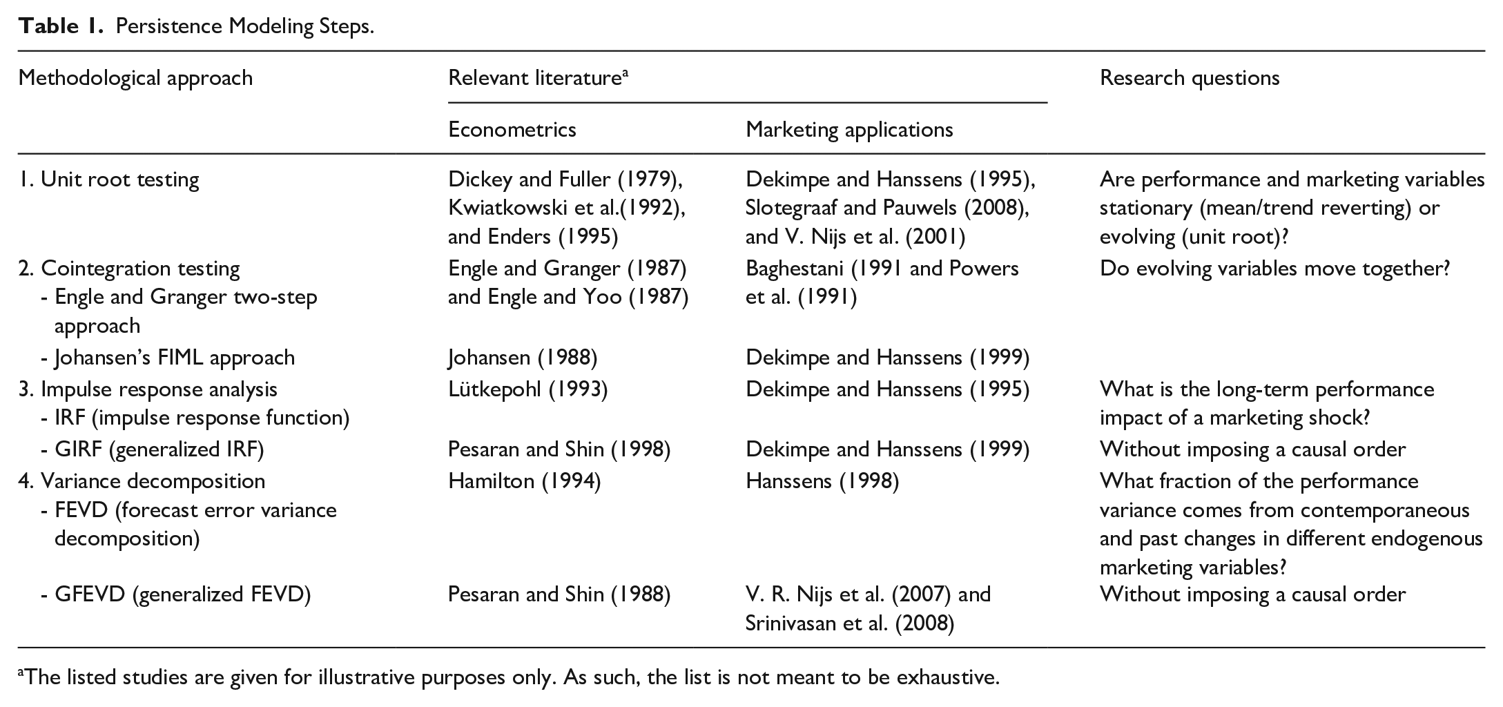
The listed studies are given for illustrative purposes only. As such, the list is not meant to be exhaustive.

IRFs can been seen as the difference between two forecasts (each over multiple periods): one based on an information set that does not take the marketing shock into account, and another based on an extended information set that takes this action into account. (Pauwels et al., 2002). As such, IRFs trace the incremental effect of the marketing action reflected in the original shock.

A stylized example is given in Figure 1.⁴ The top IRF traces the sales impact of a price-promotion shock in a mean-reverting market. The IRF shows various fluctuations over time: a positive immediate effect, followed by a typical stockpiling effect, after which some additional sales are observed that could be due to, for example, purchase reinforcement and/or firm-specific decision rules (where successful promotions lead to another price reductions). Eventually, however, any incremental effect disappears, potentially due to competitive reactions. This does not imply that the product no longer realizes any sales, but rather that no additional sales can be attributed to the initial promotion. In contrast, in the bottom panel, we see that this incremental effect stabilizes at a non-zero, or persistent, level. In that case, we have identified a long-run effect, as the initial promotion keeps on generating extra sales. Behavioral explanations for this phenomenon could be that newly attracted customers make regular repeat purchases or that the existing customer base has increased its usage rate.

Figure 1.

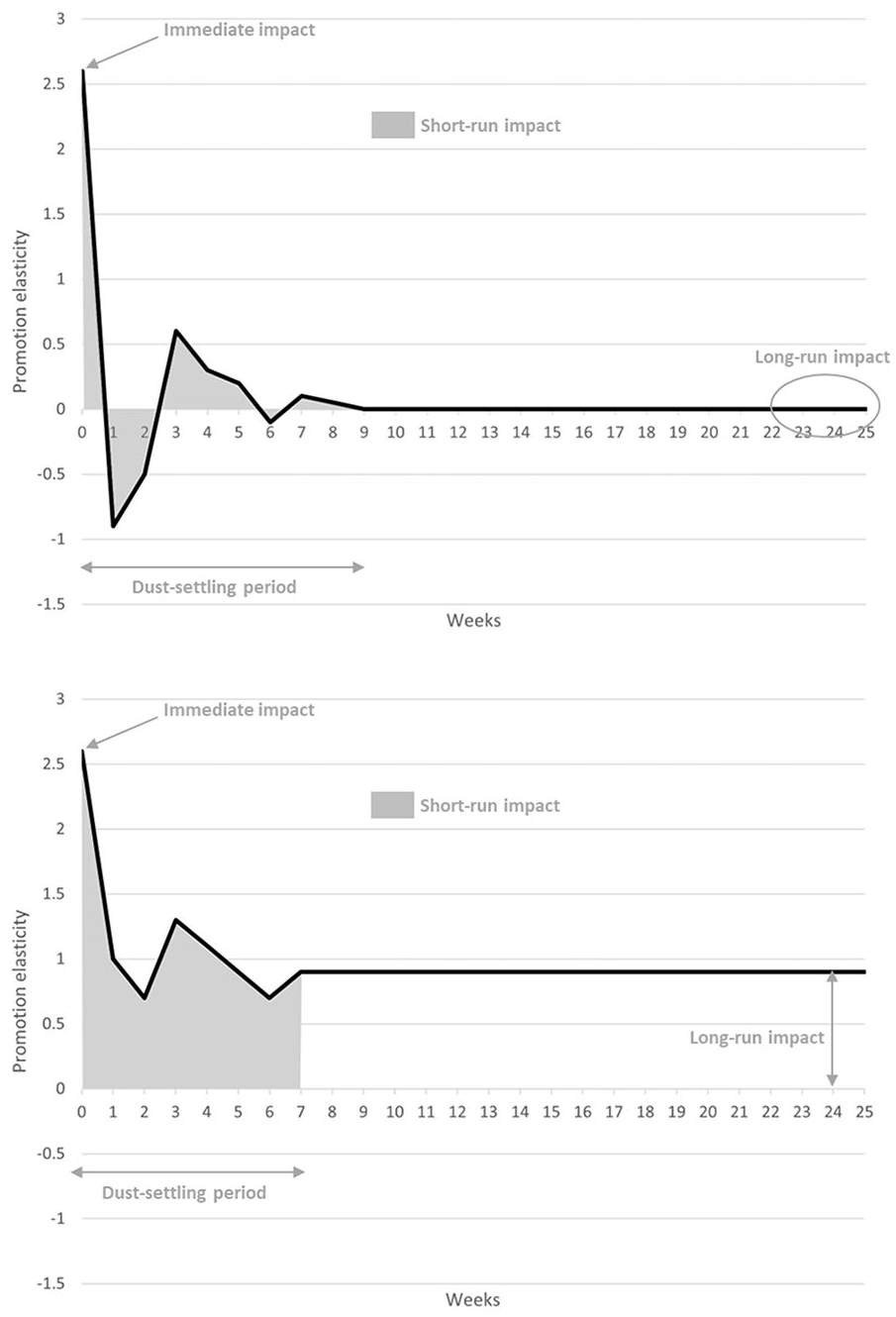
Impulse-response functions: some stylized examples.

While impulse-response functions are useful summary devices, the multitude of numbers (one per post-shock period) involved still makes them somewhat cumbersome report (unless presented in a graphical way as in Figure 1) and hard to compare across brands, markets, or marketing-mix instruments. To reduce this set of numbers to a more manageable size, one often (see, among others, Nijs et al., 2001; Nijs et al., 2007; Pauwels & Srinivasan, 2004; Srinivasan et al., 2004) derives various summary statistics from them, such as⁵:

(i) the immediate (same period) impact of the marketing shock;

(ii) the long-run or permanent (persistent) impact, which is the value to which the IRF converges;

(iii) The time interval before convergence is obtained is often referred to as the dust-settling period (Dekimpe & Hanssens, 1999; Nijs et al., 2001), and the cumulative effect over this time period is often referred to as the total short-run effect. For mean- (or trend-) reverting series, this reflects the area under the curve. In case of a persistent effect, the combined (cumulative effect) over the the dust-settling period is computed as comparable metric; and

(iv) finally, the relative importance of (current and past fluctuations in) a given marketing instrument (or other shock component) in explaining the future evolution of the performance metric can be derived through an error-variance decomposition (see, e.g. Nijs et al., 2007).

Substantive insights

Marketing-mix effectiveness

Initial applications of the persistence-modeling approach in marketing focused on the quantification of short- and long-run elasticitiess of different marketing-mix instruments on a variety of performance metrics. The marketing-mix instruments included, among others, advertising support (Dekimpe & Hanssens, 1995; van Heerde et al., 2013), price promotions (Dekimpe et al., 1999; Slotegraaf & Pauwels, 2008; Srinivasan et al., 2004), product innovations (Pauwels et al., 2004), assortments (Bezawada & Pauwels, 2013), or competitive activities (Steenkamp et al., 2005), and the performance metrics have been primary (Dekimpe et al., 1999; Nijs et al., 2001) or secondary demand (Dekimpe & Hanssens, 1995), brand and retailer revenues (Srinivasan et al., 2004), profitability (Dekimpe & Hanssens, 1999), or stock prices (Pauwels et al., 2004), among others. While many studies have focused on the aggregate performance metrics, others explored the heterogeneity in response across performance components such as category incidence, brand choice, and purchase quantity (Pauwels et al., 2002), or across consumer segments (Lim et al., 2005; Sismeiro et al., 2012). In combination, these studies have resulted in a rich set of empirical generalizations on marketing’s short- and long-run effectiveness.

Following this initial wave of studies, persistence modeling has added substantial insights to multipe research streams, among which (i) the marketing-finance interface, (ii) research on the relative effectiveness of, and inter-relationships between, numerous new/social media, and (iii) the relevance of mindset metrics to better understand the sequencing of advertising’s performance effects. A common feature across these streams are (i) the potential presence of multiple complex feedback loops with little a priori knowledge on the direction of the relationships, and (ii) an interest in disentangling the short- and long-run effects of changes in one variable on other variables in the system. Srinivasan et al. (2015), for example, considered the effects of consumer activities on paid, owned, and earned online media on sales, as well as potential feedback loops with the more traditional marketing-mix elements of price, advertising and distribution, while Hewett et al. (2016) studied how social media sites create a reverberating “echoverse” for information dissemination, involving feedback loops (“echoes”) among multiple information sources, such as corporate communications, news media, and user-generated social media. Valenti et al. (2023), in turn, considered how advertising influences how consumers think, feel, and experience a product, how different mindset metrics interact with one another and mediate advertising’s impact on sales, and how not only the size but also the sequence of these influences varied across brands and categories.

Marketing-finance interface

Time-series methods are well suited to analyze stock-price data and quantify their sensitivity to new marketing information. Not only can they be employed without having to resort to strong a priori assumptions about investor behavior such as full market efficiency, VARX models are also very flexible to accommodate feedforward and feedback loops between investor behavior and managerial behavior. Given the increasing interest in understanding the linkage between product markets (or Main Street) and financial markets (or Wall Street), it is not surprising that time-series models in general, and VAR models in particular, have been used extensively in that research domain. Chakravarty and Grewal (2011), for example, showed how managers, in response to investor expectations for short-term stock returns, may decide to modify their R&D expenditures, their marketing budgets, or both to avoid short-term earnings shortfalls, even when this results in a reduced long-run profitability. Joshi and Hanssens (2010), in turn, established that advertising can have a direct effect on firm value, beyond its indirect effect through market performance, while Luo et al. (2013) showed how variance in brand ratings across consumers (brand dispersion) hurts stock returns yet reduces firm risk. More extensive reviews on how persistence modeling has contributed to the marketing-finance interface discussion are available in Srinivasan and Hanssens (2009), Luo et al. (2012), and Edeling et al. (2021).

Social media

The emergence of new media has brought along a new set of marketing metrics, which can easily be tracked over time. Given the multitude of these new media (Twitter, Facebook, etc.), the large number of metrics that can be derived from them (like website visits, paid search clicks, Facebook likes, Facebook unlikes, etc.), and the large number of feedback loops that may exist (not only among these online metrics themselves, but also with more traditional off-line metrics), many researchers have opted for the flexibility of VAR models, with their data-driven identification of relevant effects, to study these phenomena. Trusov et al. (2009), for example, studied the effect of word-of-mouth marketing on membership growth at an online social network, and compared it with more traditional media and marketing events. Word-of-mouth referrals were found to have higher elasticities than more conventional marketing tactics. Borah and Tellis (2016) identified asymmetric halo effects where negative online chatter for one product increases negative chatter about other (own and competing) products. These halo effects were shown to subsequently affect downstream performance metrics such as sales and stock performance. Luo and Zhang (2013), in turn, linked various buzz and online traffic measures to the subsequent performance of a firm’s stock-market value. We refer to Dekimpe and Hanssens (2023) for further illustrations.

Inclusion of mindset metrics

While mind-set metrics such as awareness, liking and consideration have a long history in marketing (e.g. as building blocks in hierarchy-of-effects models), questions/doubts about their long-term sales effects through brand building have long prevailed. Not only were time-series data on these metrics often missing, prior evidence on the exact inter-relationships and sequence of these effects was mixed (Srinivasan et al., 2010). Indeed, marketing theory appears insufficiently developed to posit non-equivocally one specific sequence. A flexible modeling approach that does not impose an a priori sequence on the effects, yet which can capture multiple interactions among the various measures, was therefore called for. VAR models are ideally placed to do so, and were used in, among others, Srinivasan et al. (2010) and Pauwels and van Ewijk (2013). Srinivasan et al. (2010), for example, added, for more than 60 CPG brands, various mindset metrics to a VAR model that already accounted for the short- and long-run effects of advertising, price, distribution and promotions. Importantly, the mind-set metrics added considerable explanatory and forecasting power, and can therefore be used by managers as early performance indicators. Pauwels and Van Ewijk (2013), in turn, combine slower-moving attitudinal survey measures with rapidly-changing online behaviorial metrics to explain the sales evolution of over 30 brands across a diverse set of categories (CPG as well as services and durables).

Integrating developments across all three research streams, Colicev et al. (2018) estimated a 13-equation VAR model through which they studied the impact of owned and earned social media (OSM and ESM) on brand awareness, purchase intent, and customer satisfaction, while also linking these consumer mindset metrics to shareholder value (abnormal returns and idiosyncratic risk). Other studies in this domain are reviewed in, among others, Srinivasan (2015) and Dekimpe and Hanssens (2023).

Toward a more normative focus

The initial persistence-modeling applications in marketing tended to focus on the introduction of a new technique (e.g. unit-root testing and Impulse Response Functions in Dekimpe & Hanssens, 1995) or Generalized Impulse Response Functions (GIRFs) in Dekimpe and Hanssens (1999) or aimed to establish a superior model fit and/or forecasting performance when adding a certain type of variables (e.g. mindset metrics in Srinivasan et al., 2010). However, subsequent applications gradually started to have a more substantive (descriptive and/or hypothesis-testing) focus.

Because of a growing data availability, persistence models were increasingly estimated in a consistent way across a broad spectrum of brands and categories. This resulted in various empirical generalizations on the typical effect sizes for a variety of (short- and long-run) marketing-mix elasticities. For example, based on an analysis of 25 US categories and close to 600 Dutch CPG categories, Nijs et al. (2001) and Srinivasan et al. (2004) concluded that typical estimates of the total (long-run) price promotion elasticities are around 3.70 for brand sales, 2.30 for manufacturer revenue, 0.50 for category sales at the chain level, 1.40 for category sales at the national level, −0.05 of retailer revenue and −0.70 for retailer margins.⁶ Moreover, given the underlying multitude of elasticity estimates, studies started to add an additional modeling step to better understand the observed heterogeneity by linking them to a broad set of brand- and category-related contingency factors. Nijs et al. (2001), for example, examined to what extent price-promotions’ short- and long-run primary-demand elasticities were systematically and predictably linked to the category’s promotional depth and frequency, advertising intensity, competitive reactivity and competitive structure. As another example, Kübler et al. (2020) studied when (i.e. for which brands and industries) various sentiment extraction tools had the most explanatory and predictive power on a variety of mindset metrics. Other studies have done so in an international setting and have investigated to what extent marketing elasticities differ, for example, between emerging and developed markets (see, e.g, Pauwels et al., 2013).

These Empirical Generalizations, along with their relevant contingency factors, are not only of clear academic interest, but also offer managers a benchmarking opportunity to compare the elasticities of their own brand(s) with. Still, more actionable insights could be obtained when using the resulting elasticities to arrive at normative recommendations. Insights in the relative (short- and long-run) effectiveness of the different on- and off-line media that many brands use, for example, are essential when optimizing their media allocation decisions.

Building on a long tradition (see, e.g. Hanssens et al., 2001, Chapter 9, for a review or Leeflang et al., 2000, pp. 154–155 for a formal derivation), several studies have started to infuse persistence-based response elasticities in the Dorfman and Steiner (1954) recommendation to set optimal allocation shares in accordance to the instruments’ elasticity ratios. Kireyev et al. (2016), for example, found that a bank’s online search elasticities were significantly higher than the corresponding display elasticities, and argued that the firm should (relative to its current allocation) spend 36% more on the former and 31% less on display advertising to optimize its customer acquisition. Joshi and Hanssens (2010), in turn, used estimated long-run advertising response elasticities to derive the profit-maximizing advertising levels for two personal-computer brands, while Pauwels et al. (2016) used persistence-based elasticity estimates in combination with the Dorfman and Steiner (1954) allocation rule to show how synergy effects between different media channels can substantially alter a brand’s optimal media allocation.

More recently, Datta et al. (2022) considered the cross-country budget allocation for a leading washing-machine brand, and compared its actual allocation with (i) the allocation that would be recommended on the basis of the Dorman-Steiner elasticity-ratio rule, and (ii) the improved optimal allocation rule of Fischer et al. (2011) that not only the takes the market responsiveness into account (which they obtained from an error-correction specification) but also the size of each country’s profit contribution (last year’s sales × profit contribution) along with its growth potential over a given planning horizon.

Conclusion

We see an increasing use of time-series models in the academic marketing literature, not only because more extensive (in terms of both the included variables and the length of the time window covered) data sets become available combined with a growing openness to data-driven Empirics-First research (Golder et al., 2023), but also because various research questions have come to the fore that (i) potentially/likely involve multiple feedback loops, and where (ii) marketing theory is insufficiently developed to specify a priori all temporal precedence relationships. In those instances, the flexibility of VAR models to capture dynamic inter-relationships, and to the ability of persistence modeling to quantify the short- and long-run effects of the various influences at hand, becomes very valuable.

Moreover, by combining the resulting short- and long-run effectiveness estimates with some well-known optimal allocation rules as developed by Dorfman and Steiner (1954) and extended in Fischer et al. (2011), the managerial insights and recommendations have become more actionable. In line with that evolution, persistence-modeling has seen a growing acceptance in practice as well. A non-exhaustive list of companies/brands that have already made use of persistence modeling to support their decision making include Amazon, Bank of America, Heineken, L’Occitane, Nissan Motor, Sony, Tetra Pak, Unilever, Vistaprint, and World Education Services.⁷

We are hopeful to see a further diffusion of these techniques in the academic and business marketing communities in the years to come.

Footnotes

Acknowledgements

The authors thank the participants of the 2023 Marketing Analytics Symposium Sidney (MASS) for useful comments on the ideas presented in the manuscript.

Declaration of conflicting interests

The author(s) declared no potential conflicts of interest with respect to the research, authorship, and/or publication of this article.

Funding

The author(s) received no financial support for the research, authorship, and/or publication of this article.

ORCID iD

Marnik G. Dekimpe

Notes

References

Baghestani

(1991). Cointegration analysis of the advertising-sales relationship. Journal of Industrial Economics, 39(6), 671–681.

Bass

F. M.

Clarke

D. G.

(1972). Testing distributed lag models of advertising effect. Journal of Marketing Research, 9(3), 298–308.

Bezawada

Pauwels

(2013). What is special about marketing organic products? How organic, price and promotions drive retailer performance. Journal of Marketing, 77(1), 31–51.

Borah

Tellis

G. J.

(2016). Halo (spillover) effects in social media: Do product recalls of one brand hurt or help rival brands? Journal of Marketing Research, 53(2), 143–160.

Chakravarty

Grewal

(2011). The stock market in the driver’s seat! Implications for R&D and marketing. Management Science, 57(9), 1594–1609.

Colicev

Malshe

Pauwels

O’Connor

(2018). Improving consumer mindset metrics and shareholder value through social media: The different roles of owned and earned media. Journal of Marketing, 82(1), 37–56.

Dalrymple

D. J.

(1987). Sales forecasting practices: Results from a United States survey. International Journal of Forecasting, 3(3–4), 379–391.

Datta

van Heerde

H. J.

Dekimpe

M. G.

Steenkamp

J.-B. E. M

. (2022). Cross-national differences in market response: Line-length, price, and distribution elasticities in fourteen Indo-Pacific Rim economies. Journal of Marketing Research, 59(2), 251–270.

Dekimpe

M. G.

Hanssens

D. M.

(1995). The persistence of marketing effects on sales. Marketing Science, 14(1), 1–21.

10.

Dekimpe

M. G.

Hanssens

D. M.

(1999). Sustained spending and persistent response: A new look at long-term marketing profitability. Journal of Marketing Research, 36(4), 397–412.

11.

Dekimpe

M. G.

Hanssens

D. M.

(2000). Time-series models in marketing: Past, present and future. International Journal of Research in Marketing, 17(2-3), 183–193.

12.

Dekimpe

M. G.

Hanssens

D. M.

(2010). Time series models in marketing: Some recent developments. Marketing - Journal of Research and Management, 6(1), 93–98.

13.

Dekimpe

M. G.

Hanssens

D. M.

(2023). Persistence modeling in marketing: From a descriptive and predictive focus to normative uses. In Mizik

Hanssens

D. M.

(Eds.) Handbook of marketing analytics: Methods and applications in marketing management, public policy and litigation support (2nd ed.). Edward Elgar.

14.

Dekimpe

M. G.

Hanssens

D. M.

Silva-Risso

J. M.

(1999). Long-run effects of price promotions in scanner markets. Journal of Econometrics, 89(1–2), 269–291.

15.

Dickey

D. A.

Fuller

W. A.

(1979). Distribution of the estimators for autoregressive time series with a unit root. Journal of the American Statistical Association, 74(366), 427–731.

16.

Dorfman

Steiner

P. O.

(1954). Optimal advertising and optimal quality. American Economic Review, 4, 826–836.

17.

Edeling

Srinivasan

Hanssens

D. M.

(2021). The marketing-finance interface: A new integrative review of metrics, methods, and findings, and an agenda for future research. International Journal of Research in Marketing, 38(4), 857–876.

18.

Enders

(1995), Applied econometric time series. John Wiley & Sons.

19.

Engle

R. F.

Granger

C. W J.

(1987). Cointegration and error correction: Representation, estimation and testing. Econometrica, 55(2), 251–276.

20.

Engle

R. F.

Yoo

B. S.

(1987). Forecasting and testing in co-integrated systems. Journal of Econometrics, 35(1), 143–159.

21.

Fischer

Albers

Wagner

Frie

(2011). Dynamic marketing budget allocation across countries, products, and marketing activities. Marketing Science, 30(4), 568–585.

22.

Franses

P. H.

(2001). How to deal with intercept and trend in practical cointegration analysis. Applied Economics, 33(5), 577–579.

23.

Golder

P. N.

Dekimpe

M. G.

J. T.

van Heerde

H. J.

Kim

D. S. U.

Alba

J. W.

(2023). Learning from data: An empirics-first approach to relevant knowledge generation. Journal of Marketing, 87(3), 319–336.

24.

Granger

C. W. J.

(1981). Some properties of time series data and their use in econometric model specification. Journal of Econometrics, 16(1), 121–130.

25.

Hamilton

(1994). Time series analysis. Princeton University Press.

26.

Hanssens

D. M.

(1988). Order forecasts, retail sales and the marketing mix for consumer durables. Journal of Forecasting, 17(3/4), 327–346.

27.

Hanssens

D. M.

(2015). Empirical generalizations about marketing impact. Marketing Science Institute.

28.

Hanssens

D. M.

Dekimpe

M. G.

(2012). Short-term and long-term effects of marketing strategy. In Shankar

Carpenter

(Eds.), Handbook of marketing strategy (pp. 457–469). Edward-Elgar Publishing.

29.

Hanssens

D. M.

Parsons

L. J.

Schultz

R. L.

(2001). Market response models. Kluwer Academic Publishers.

30.

Hewett

Rand

Rust

R. T.

van Heerde

H. J.

(2016). Brand buzz in the echoverse. Journal of Marketing, 80(3), 1–24.

31.

Homburg

Klarmann

Vomberg

(2021). Handbook of market research. Springer Nature.

32.

Johansen

(1988). Statistical analysis of cointegration vectors. Journal of Economic Dynamics and Control, 12(2–3), 231–254.

33.

Joshi

A. M.

Hanssens

D. M.

(2010). The direct and indirect effects of advertising spending on firm value. Journal of Marketing, 74(1), 20–33.

34.

Kireyev

Pauwels

Gupta

(2016). Do display ads influence search? Attribution and dynamics in online advertising. International Journal of Research in Marketing, 33, 475–490.

35.

Kübler

R. V.

Colicev

Pauwels

K. H.

(2020). Social media’s impact on the consumer mindset: When to use which sentiment extraction tool? Journal of Interactive Marketing, 50, 136–155.

36.

Kwiatkowski

Phillips

P. C. B.

Schmidt

Shin

(1992). Testing the null hypothesis of stationarity against the alternative of a unit root. Journal of Econometrics, 54(1–3), 159–178.

37.

Leeflang

P. S. H.

Wittink

D. R.

(1992). Diagnosing competitive reactions using (aggregated) scanner data. International Journal of Research in Marketing, 9(1), 39–57.

38.

Leeflang

P. S. H.

Wittink

D. R.

(1996). Competitive reaction versus consumer response: Do managers overreact? International Journal of Research in Marketing, 13(2), 103–119.

39.

Leeflang

P. S. H.

Wittink

D. R.

Wedel

Naert

P. A.

(2000). Building models for marketing decisions. Kluwer Academic Publishers.

40.

Lim

Curim

I. S.

Andrews

R. L.

(2005). Consumer heterogeneity in the longer-term effects of price promotions. International Journal of Research in Marketing, 22(4), 441–457.

41.

Luo

Pauwels

K. H.

Hanssens

D. M.

(2012). Time-series models of pricing the impact of marketing on firm value. In Ganesan

(Ed.), Handbook of marketing and finance (pp. 43–65). Edward Elgar.

42.

Luo

Raithel

Wiles

M. A.

(2013). The impact of brand rating dispersion on firm value. Journal of Marketing Research, 50(3), 399–415.

43.

Luo

Zhang

(2013). How do consumer buzz and traffic in social media marketing predict the value of the firm? Journal of Management Information Systems, 30(2), 213–238.

44.

Lütkepohl

(1993). Introduction to multiple time series analysis. Springer-Verlag.

45.

Nijs

Dekimpe

M. G.

Steenkamp

J.-B. E. M.

Hanssens

D. M.

(2001). The category demand effects of price promotions. Marketing Science, 20(1), 1–22.

46.

Nijs

V. R.

Srinivasan

Pauwels

(2007). Retail-price drivers and retailer profits. Marketing Science, 26(4), 473–487.

47.

Pauwels

(2018). Modeling dynamic relations among marketing and performance metrics. Foundations and Trends® in Marketing, 11(4), 215–301.

48.

Pauwels

Demirci

Yildirim

Srinivasan

(2016). The impact of brand familiarity on online and offline media synergy. International Journal of Research in Marketing, 33(4), 739–753.

49.

Pauwels

Erguncu

Yidirim

(2013). Winning hearts, minds and sales: How marketing communication enters the purchase process in emerging and mature markets. International Journal of Research in Marketing, 30(1), 57–68.

50.

Pauwels

Hanssens

D. M.

Siddarth

(2002). The long-term effects of price promotions on category incidence, brand choice and purchase quantity. Journal of Marketing Research, 39(4), 421–439.

51.

Pauwels

Silva-Risso

Srinivasan

Hanssens

D. M.

(2004). New products, sales promotions, and firm value: The case of the automobile industry. Journal of Marketing, 68(4), 142–156.

52.

Pauwels

van Ewijk

(2013). Do online behavior tracking or attitude survey metrics drive brand sales? An integrative model of attitudes and actins on the consumer boulevard (Marketing Science Institute Working Paper Series No. 13–118). Marketing Science Institute.

53.

Pauwels

Srinivasan

(2004). Who Benefits from Store Brand Entry? Marketing Science, 23(3), 364–390.

54.

Pesaran

H. H.

Shin

(1998). Generalized impulse response analysis in linear multivariate models. Economic Letters, 58(1), 17–29.

55.

Powers

Hanssens

D. M.

Hser

Y.-I.

Anglin

M. D.

(1991). Measuring the long term effects of public policy: The case of narcotics use and property crime. Management Science, 37(6), 627–644.

56.

Sismeiro

Mizik

Bucklin

R. E.

(2012). Modeling coexisting business scenarios with time-series panel data: A dynamics-based segmentation approach. International Journal of Research in Marketing, 29(2), 134–147.

57.

Slotegraaf

R. J.

Pauwels

(2008). The impact of brand equity and innovation on the long-term effectiveness of promotions. Journal of Marketing Research, 45(3), 293–306.

58.

Srinivasan

. (2015). Customer mindset metrics and firm performance. In Kumar

Shah

(Eds.) Handbook of research on customer equity in marketing (pp. 306–332). Edward Elgar Publising.

59.

Srinivasan

(2021). Modeling marketing dynamics using vector autoregressive (VAR) models. In Homburg

Klarmann

Vomberg

(Eds.) Handbook of market research (pp. 515–547). Springer.

60.

Srinivasan

Hanssens

D. M.

(2009). Marketing and firm value: Metrics, methods, findings and future directions. Journal of Marketing Research, 46(3), 293–312.

61.

Srinivasan

Pauwels

Hanssens

D. M.

Dekimpe

M. G.

(2004). Do promotions benefit manufacturers, retailers, or both? Management Science, 50(5), 617–629.

62.

Srinivasan

Pauwels

Nijs

(2008). Demand-based pricing versus past-price dependence: A cost-benefit analysis. Journal of Marketing, 72(2), 15–27.

63.

Srinivasan

Rutz

O. J.

Pauwels

(2015). Paths to and off purchase: Quantifying the impact of traditional marketing and online consumer activity. Journal of the Academy of Marketing Science, 44, 440–453.

64.

Srinivasan

Vanhuele

Pauwels

(2010). Mind-set metrics in market response models: An integrative approach. Journal of Marketing Research, 47(4), 672–684.

65.

Steenkamp

J.-B. E. M.

Nijs

V. R.

Hanssens

D. M.

Dekimpe

M. G.

(2005). Competitive reactions to advertising and promotion attacks. Marketing Science, 24(1), 35–54.

66.

Trusov

Bucklin

R. E.

Pauwels

(2009). Effects of word-of-mouth versus traditional marketing: Findings from an internet social networking site. Journal of Marketing, 73(5), 90–102.

67.

Valenti

Yildirim

Vanhuele

Srinivasan

Pauwels

(2023). Advertising’s sequence of effects on consumer mindset and sales: A comparison across brands and product categories. International Journal of Research in Marketing, 40(2), 435–454.

68.

van Heerde

H. J.

Gijsenberg

Dekimpe

M. G.

Steenkamp

J.-B. E. M

. (2013). Price and advertising effectiveness over the business cycle. Journal of Marketing Research, 50(2), 177–193.

69.

Wang

Yildirim

(2021). Applied time-series analysis in marketing. In Homburg

Klarmann

Vomberg

(Eds.) Handbook of market research (pp. 469–513). Springer.

70.

Winklhofer

Diamantopoulos

Witt

S. F.

(1996). Forecasting practice: A review of the empirical literature and an agenda for future research. International Journal of Forecasting, 12, 193–221.

Persistence Modeling in Marketing: Descriptive,Predictive,and Normative Uses

Abstract

Keywords

Time series data and time series models

Persistence modeling

Substantive insights

Marketing-mix effectiveness

Marketing-finance interface

Social media

Inclusion of mindset metrics

Toward a more normative focus

Conclusion

Footnotes

Acknowledgements

Declaration of conflicting interests

Funding

ORCID iD

Notes

References