Sage Journals: Discover world-class research

Abstract

Natural ventilation is a highly respected and effective way to improve indoor air quality, and single-sided natural ventilation is easily formed in residential buildings. The site experiments were carried out, and the unsteady characteristics of the airflow were analyzed based on 3D wind speed series. With the experimental verification, large-eddy simulation was successfully applied to calculate the indoor–outdoor flow field of urban building groups. When the entrance boundary was constant, the flow field of the window varied all the time, and outflow was irregular. The natural ventilation efficiency was 42% with the incoming flow almost parallel to the window. The discrete wind speed inlet boundary is more suitable for the natural ventilation simulation of buildings in a real environment than the average wind speed boundary and the average wind speed superposition ±10% disturbance.

Keywords

Single-sided natural ventilation unsteady characteristics experimental measurement large-eddy simulation urban building groups

Introduction

Because of the COVID-19 outbreak, people are spending more time indoors.¹ Natural ventilation is of great significance in preventing the spread of aerosol-transmitted diseases indoors.^2–5 A survey of window-opening habits of Chinese residents revealed that 86.8% of the residents chose single-sided ventilation in northern China.⁶ Therefore, single-sided natural ventilation is an important ventilation mode for residential buildings,^7,8 and it can create a healthy and comfortable indoor environment.⁹

Numerical simulation facilitates the study of urban building ventilation.^10,11 By far, the two popular models in building simulation are based on Reynolds-averaged Navier–Stokes (RANS) equations and large-eddy simulation (LES).^12–15 The RANS model has a long history of application, with wide use in the calculation of mean flow field. With an appropriate turbulence model and numerical conditions, the prediction accuracy is acceptable. However, it cannot simulate the transient flow field and is limited in some applications.^16,17 Meanwhile, LES requires significant computational power, but the potential accuracy of LES is clearly superior.¹⁸ LES can provide a more detailed prediction of the airflow at building openings (which is important for natural ventilation),¹⁹ as well as the turbulence nature and pollutant distribution.^16,20,21 LES has been widely employed to study flow past an isolated cubic building,^22,23 flow within the regular and irregular obstacle arrays^24,25 and actual urban areas.^26–28 However, few studies have directly coupled indoor and outdoor flow fields for simulation. For the LES and RANS simulation of indoor and outdoor flow fields, the RANS model was not sufficiently accurate to simulate the pollutant diffusion around multistorey buildings.⁷ However, the study focused on a single building. The dynamic characteristics of natural ventilation directly affect the pulsating propagation of pollutants. Therefore, LES is more suitable for the single-sided numerical simulation of unsteady natural ventilation in a real environment.¹⁹ Meanwhile, both the RANS and LES models involve wind-tunnel tests and simulations for a single building, whereas numerous scholars have demonstrated that the presence of surrounding building groups affects the flow field around the target residence.^29–31 Urban ventilation simulation usually accounts for the influence of surrounding buildings, but not in relation to the flow field indoors.³² Some scholars^33,34 simulated the airflow both indoors and outdoors in a building group, but the indoor and outdoor flow fields were conducted separately.

Therefore, studies of indoor and outdoor flow fields under natural ventilation with LES considered the influence of surrounding buildings in an urban residential setting simultaneously was not perfect. There is no unified standard or guide for large-eddy simulation in building simulation.¹² The average wind speed³⁵ or the average wind speed with a certain proportion of disturbance, such as 10%¹⁹, is usually used as an inlet boundary. The discrete wind speed obtained from experiments can also be used as an inlet boundary in building simulations. However, which method is more suitable for large-eddy simulations of real buildings has not been identified.

In this investigation, on-site measurement in urban building groups with single-sided natural ventilation was carried out, and the unsteady characteristics of the flow field were analyzed. A large-eddy simulation was successfully applied to calculate the indoor and outdoor flow fields considering the surrounding building groups and was verified by experiments. Furthermore, the instantaneous flow characteristics at the window and the ventilation efficiency of single-sided natural ventilation were explored, and the above three inlet velocity setting methods in indoor and outdoor simulation of real environment buildings were compared.

Field measurement

Due to the unsteady characteristics of natural ventilation in real environments, field measurement data in urban building groups is not enough. In this study, synchronous measurement of indoor and outdoor flow fields was conducted in an apartment located in Tianjin, China. Two HOBO micro weather stations were installed 2 m above the rooftop of the building (18 m from the ground) for measurement of outdoor environmental parameters as shown in Figure 1(a). When the measured wind speed was greater than 0.5 m/s, the wind speed measurement accuracy of the micro weather station was ±4%, the accuracy of wind direction measurement was ±5° and the accuracy of air temperature measurement was ±0.2°C. Measurement of wind speed and wind direction provided boundary conditions for the simulation. The building and the layout of the single-sided naturally ventilated room can be found in Figure 1(a). To ensure single-sided natural ventilation, we sealed the door of the ventilated room to separate it from other rooms. Three 3D ultrasonic anemometers were evenly arranged along the vertical centreline of the window as shown in Figure 1(b). The operational accuracy of the anemometers was ± (2% + 0.03 m/s of the absolute value of the indicated value), and the measurement frequency was 20 times per second. The test window faced south, and the dimensions of the opening and the measuring point coordinates are provided in Figure 1(b). The measurement of the wind speed series provided a basis for the subsequent grid size and time step calculation and turbulence characteristics analysis.

Figure 1.

(a) The ventilated apartment and (b) the dimensions of the window and the locations of three ultrasonic anemometers.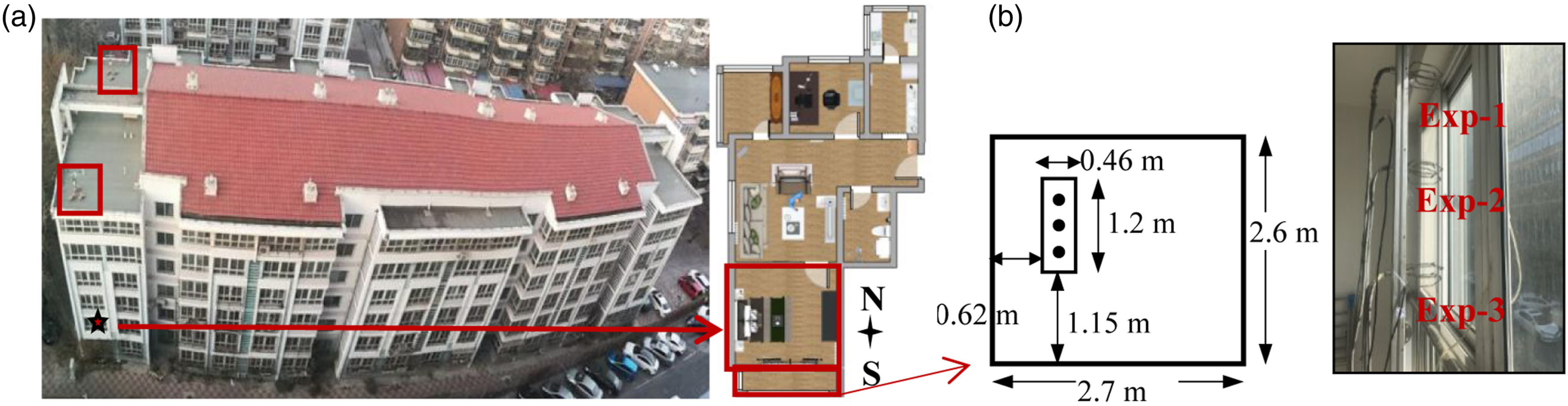

At the same time, the single-sided natural ventilation rate was measured by the carbon dioxide tracer gas attenuation method. This investigation sealed all the openings at the beginning of the experiment. Carbon dioxide as the tracer gas was released into the room and a fan was used to enhance the mixing in the middle of the bedroom until the CO₂ concentration was at least 3500 ppm higher than the outdoor concentration. The fan was then switched off, and a window was opened for single-sided ventilation. During the experiment, the indoor and outdoor carbon dioxide concentrations were monitored simultaneously. An experiment verified that there was no significant difference in the measurement results of the ventilation rate of six measuring locations.³⁶ The indoor ventilation rate was measured at a sampling position. Carbon dioxide was used to represent an indoor contaminant, to enable comparison of experimental data with large-eddy simulation of contaminant transmission in urban building groups.

Large-eddy simulation

Computational domain and grid

The building groups surrounding the target residence could directly affect the accuracy of the simulation results for the flow field. Liu et al.³⁰ found that incorporating detailed building structures around the target building within a distance equal to three times the maximum building height would provide a reliable simulation of the flow field. As shown in Figure 2(a), the surrounding detailed buildings were circled by the white rectangle and our computational domain was 1.48 km (x direction) × 1.35 km (y direction) × 0.5 km (z direction) as shown by the red rectangle. For an external domain without detailed buildings, the extended distance is the maximum value of 5 times of the building height. The geometric model of the target building and its surrounding buildings was obtained from Google Maps. Figure 2(b) shows the target building model and the interior layout of the ventilated room, which included a bed, bedside table, wardrobe and balcony. These were exactly the same as for the experimental room.

Figure 2.

(a) Computational domain and (b) models of the target building and ventilated room.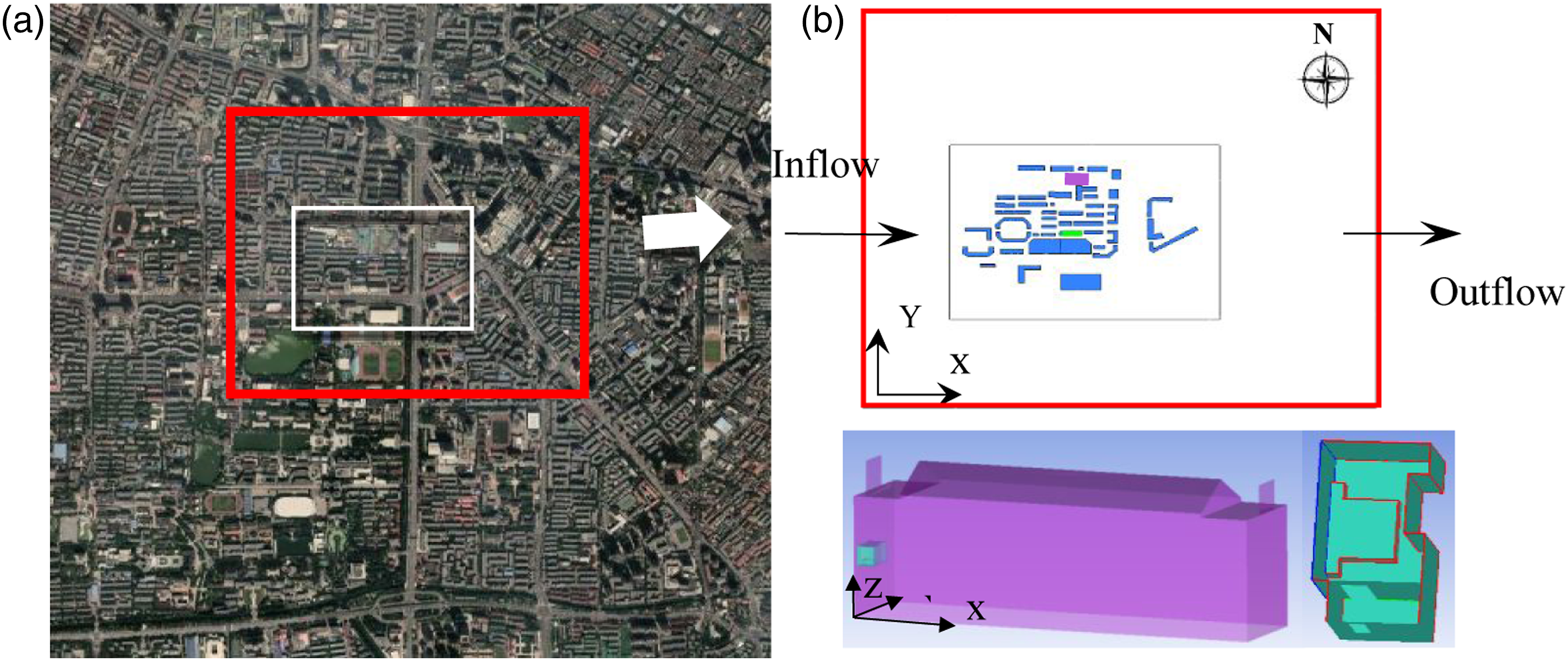

Gambit 2.4.6 was used to generate a discrete grid in this study. According to a grid sensitivity analysis in the Results section, when the number of grids reached above 6.06 million, the calculation results were relatively insensitive to the grid number. Then this study used 6.06 million grids for subsequent simulation, and the local grid distribution is shown in Figure 3. In previous simulations of actual urban areas,^26,28,33 the smallest cell sizes of LES computation were 0.2 m, 0.22 m and 0.04 m separately. Figure 3 shows the grid distribution in the interior area of the computational domain with detailed buildings, around the target building and the ventilated room. The grid size for the window and indoor space of the ventilated room was 0.05 m according to the dissipative and integral time scale based on the measured wind speed series perpendicular to the window, calculated by the formulae given in the reference.³⁷ The value of y-plus of the interior wall of the ventilated room is about 15–55. The meshes were clearly too coarse to resolve the laminar viscous layer, and the wall-adjacent cells mainly fell within the logarithm of the boundary layer. Therefore, the default LES near-wall treatment in Fluent was employed based on the work of Werner and Wengle.³⁸ The grid transition within 2 m around the target residence was implemented, as shown in Figure 3(b), especially on the ventilation window side. The grid sizes on the surfaces of the target building and the surrounding building were 0.5 m and 2 m respectively, which were increased at a ratio of 1.2. For the interior area in Figure 3(a), the grid was increased from 2 m (building surfaces) to 8 m (close to non-building areas) at a ratio of 1.02.

Figure 3.

Grid distribution around detailed building models, the target building and the ventilated room.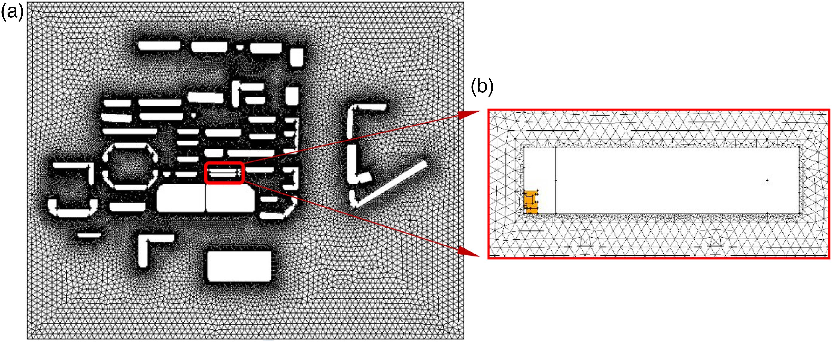

Boundary conditions

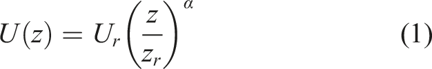
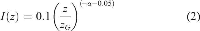
The upper surface and the north and south surfaces of the computational domain were symmetry boundaries. The surface of the ground and the buildings in the computational domain were set as non-slip walls. The inlet and outlet boundaries were velocity inlet and outflow. Since the nearest national meteorological station was 10 km away from the experiment site, this investigation used the wind speed measured by the weather station on the roof of the residence as the inlet boundary (with the same atmospheric boundary layer parameters). Some scholars³⁹ also used the meteorological parameters of the building roof as the entrance boundary. The measurement frequency of the station was once per minute. Because of the high demands of large-eddy simulation on computation hardware, the real time of 5 min needed to be calculated on a 64-core server for 7.5 days. The time step was set to 0.02 s, and the grid scale was 0.05 m according to the time scale calculation of the measured wind speed magnitude series, which was confirmed by experiments. Based on the measured wind speed series at the window, the velocity ranged 0–2.3 m/s. The range of CFL numbers was 0–0.92, which was calculated by its definition of the ratio of fluid motion distance to grid length within a time step. The Cell Convective Courant Number from simulation results at the window was between 0.32 and 1.65 with an average value of 0.93. Therefore, this study presents the calculation results based on time steps of 0.02 s for a period of 5 min to obtain the ventilation rate and reveal the unsteady characteristics of single-sided natural ventilation. The experiment was carried out on 22 March 2017. The wind speeds during these 5 min were 2.77 m/s, 2.01 m/s, 1.51 m/s, 2.27 m/s and 2.27 m/s. The wind direction affects the flow field and pollutant propagation, but this study simulated the period when the wind direction was stable and ignored the fluctuation of wind directions. The average wind direction was 275° basically unchanged in 2 hours according to data from the national weather station, which was within the dominant wind-direction range for Tianjin in this season. The wind direction angle was equal to the clockwise angle between the incoming wind speed and the north direction. At the centre of a large city, the inlet wind speed follows the power function along the height⁴⁰ with a power exponent of 0.33 (ASHRAE Handbook, 2009), as shown in Equation (1).

At present, there are two other methods to set the wind speed at the inlet boundary of large-eddy simulation of building ventilation, the average velocity³⁵ and the average value superposing random perturbations with an intensity of, u´/U, 10%.¹⁹ Including fluctuating wind speed inlet boundary, the accuracy of the three setting methods of inlet boundaries was compared in the results. Because the inlet wind speed was constant, the vortex method was chosen to determine the fluctuating velocity algorithm, and the vortex number was 300. Then in the turbulence dialog box, the k-epsilon method was selected for the specification method. The turbulence intensity, $I (z)$ , was determined by Equation (2). The vortex method requires k-epsilon information as shown in Equations (3) and (4) to generate the pulsating inlet velocity boundary based on the average velocity per minute. Corresponding to the power exponent distribution of velocity, the turbulence kinetic energy (k) and turbulent dissipation rate (ɛ) were calculated by the formula recommended by the Architectural Institute of Japan,⁴¹ which varied with the measured discrete velocity. The vertical profiles of k (m²/s²) and ɛ (m²/s³) are described by Equations (2)–(4).

U (z) = U_{r} {(\frac{z}{z_{r}})}^{α}

(1)

I (z) = 0.1 {(\frac{z}{z_{G}})}^{(- α - 0.05)}

(2)

k (z) = {(I (z) U (z))}^{2}

(3)

ε (z) = C_{μ}^{1 / 2} k (z) \frac{d U (z)}{d z}

(4)

where

U (z)

is the wind speed at the height of z, m/s;

U_{r}

is the wind speed at the reference height

z_{r}

, m/s;

α

is a power exponent related to the terrain;

I (z)

is the turbulence intensity;

z_{G}

is the atmospheric boundary layer thickness, equal to 460 in large city centres;

σ_{u} (z)

is the RMS value of the velocity fluctuation; and

C_{μ}

is the model constant (= 0.09).

CFD model

The basic theory of large-eddy simulation of turbulence fluctuation is divided into two parts through the introduction of appropriate corresponding spatial filtering technology. The large-scale fluctuation is obtained by solving the filtered Navier–Stokes equations, while the influence of small-scale fluctuation on the flow field is determined through the construction of a sub-grid scale model generated by filtering. The filtered Navier–Stokes equation is described by Equations (5) and (6):

\frac{\partial (\bar{u_{i}})}{\partial t} + \frac{\partial (\bar{u_{i}} \bar{u_{j}})}{\partial x_{j}} = - \frac{1}{ρ} \frac{\partial \bar{P}}{\partial x_{i}} + υ \frac{\partial^{2} \bar{u_{i}}}{\partial x_{j} \partial x_{j}} - \frac{\partial (\bar{u_{i} u_{j}} - \bar{u_{i}} \bar{u_{j}})}{\partial x_{j}}

(5)

\frac{\partial \bar{u_{i}}}{\partial x_{i}} = 0

(6)

where

\bar{u_{i}}

and

\bar{u_{j}}

are the components of the filtered velocity vector in the

x_{i}

and

x_{j}

directions,

ρ

is the air density,

P

is the air pressure,

υ

is the kinetic viscosity and

- (\bar{u_{i} u_{j}} - \bar{u_{i}} \bar{u_{j}})

is the anisotropic part of the sub-grid Reynolds stresses.

τ_{i j}

is the momentum transferred between filtered small- and large-scale oscillations.

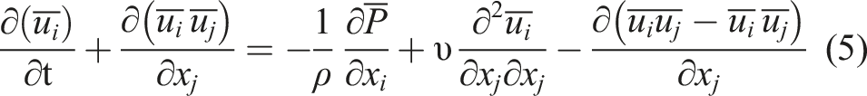
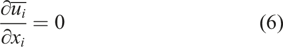
The sub-grid scale Reynolds stresses render the filtered NS equation not closed. The closure method proposed by Joseph Smagorinsky⁴² was used in this investigation which has been widely applied to airflow around and in buildings.^26,33 We conducted simulation calculations using Fluent 19.2. The Smagorinsky–Lilly model was adjusted with the Smagorinsky constant Cs = 0.12. The SIMPLE algorithm was used for the pressure velocity coupling. A second-order scheme was set for pressure and a bounded-central-differencing scheme was for momentum. For transient formulation, bounded second-order implicit was chosen. For the spread of tracer gas from indoor to outdoor environment, the species model was employed in this study, and it was confirmed to be reasonably accurate for airborne contaminants.^43,44 The RANS results were taken as the initial flow field. The concentration of carbon dioxide in the room at the beginning of LES calculation was set according to the concentration measured at the corresponding ventilation time.

Results and discussion

The field measurement results of single-sided natural ventilation and the unsteady characteristics reflected by the experimental data were analyzed. The grid sensitivity analysis and model validation are presented. Based on the simulation, the characteristics of instantaneous airflow at the window were reproduced. The ventilation efficiency of single-side natural ventilation was calculated, and different inlet boundary setting methods were compared.

Measurement results

The flow state of single-sided natural ventilation was complex at the window, including both inflow and outflow, but there was little field measurement data available. Figure 4 depicts the wind speed series perpendicular to the window from the three ultrasonic anemometers at the ventilated window. The number of measuring points is consistent with that in Figure 1(b), and the wind speed direction was positive for inflow. We found that the wind speed at Exp-1 in the upper part of the window was mostly negative, which indicated outflow. While the direction at Exp-2 and Exp-3 was the fluctuating, mainly positive, with both positive and negative wind speeds in the lower half of the window fluctuating. Namely, the upper part of the window had outward airflow, and the middle and lower parts mainly flowed in with unsteady airflow, and sometimes the wind of these measuring points turned in the opposite direction.

Figure 4.

Wind speed series perpendicular to the window measured by 3D ultrasonic anemometers.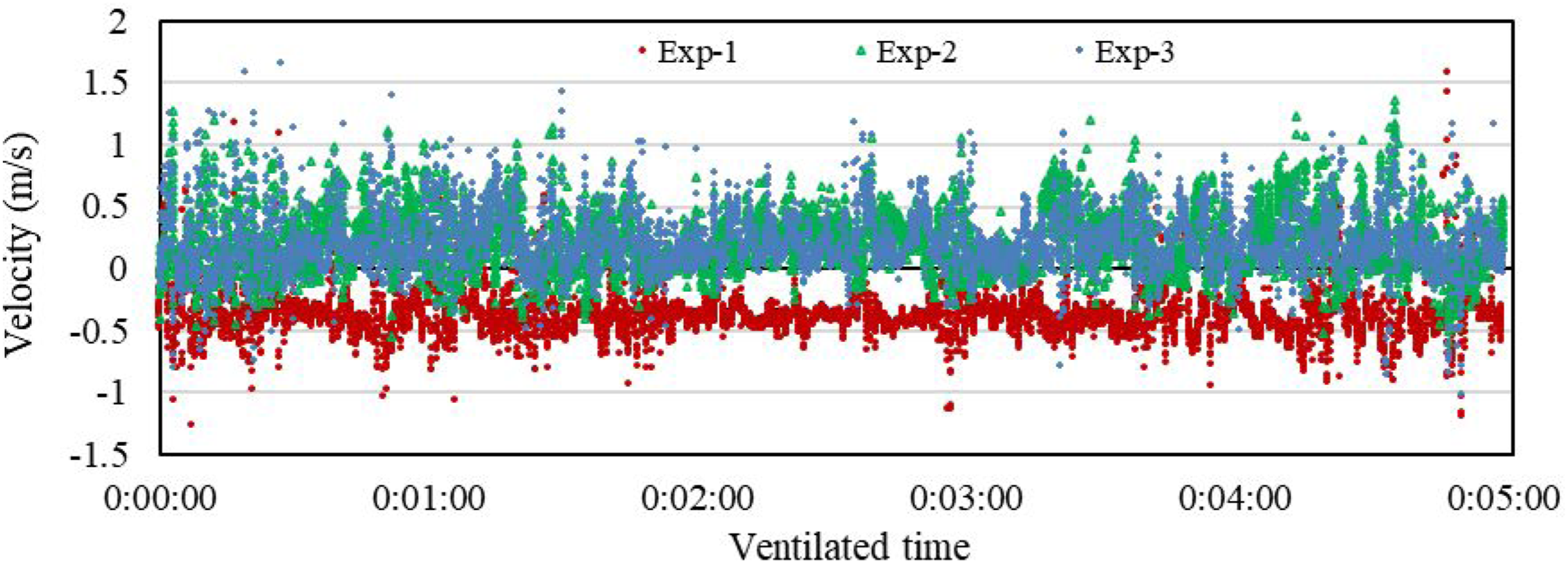

In this period, the average velocities perpendicular to the window in the three experiments were −0.39 m/s, 0.21 m/s and 0.19 m/s with a ventilation rate of 3.9 h⁻¹. Due to the overlap of speeds, we analyzed the second-order statistics for the measured turbulence characteristics, turbulence intensity and turbulence kinetic energy in Figure 5 based on wind speed series in Figure 4. As shown in Figure 5, the turbulence intensity of Exp-2 was the largest, 74%, which means that the fluctuation in the middle of the window was the most intense. The turbulence at measuring points 1 and 3 were relatively weak, 36% and 64%, respectively. However, the turbulence kinetic energy of Exp-3 and Exp-2 was similar. This indicates that there was a strong pulsation in the middle and lower parts of the window. Combined with the above wind speed analysis, the energy of the inflow air in the middle and lower parts was relatively high.

Figure 5.

Box graphs of turbulence intensity and turbulence kinetic energy at the three measuring points in a 5-minute period.

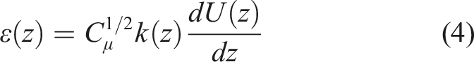
Because it is impossible to measure all the information of the flow field at the window, we calculated the scale of the vortex turbulence at the limited measuring locations based on the method given in the literature.³⁷ The calculation equations are as given in Equations (7) and (8):

I s s = I t s \times \bar{V}, I t s = \int_{0}^{+ \infty} f (r) d r

(7)

D s s = {(v^{3} / 〈 ε 〉)}^{1 / 4}, 〈 ε 〉 = 15 ν 〈 {(\partial V / \partial x)}^{2} 〉

(8)

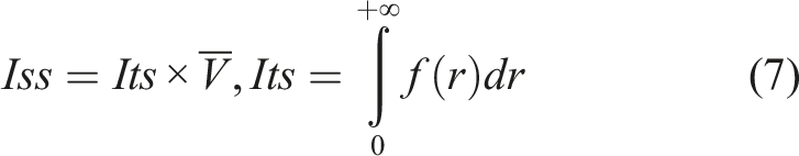
The calculated integral scale (Iss) and Kolmogorov scale (Dss) at the window were 95 mm and 0.7 mm, respectively, based on the wind speed series perpendicular to the window direction. It means that the grid scale at the window in LES in the real environment needs to be between 0.7 mm and 95 mm. Our grid size at the window and indoors in this investigation was 50 mm.

For the airflow fluctuation, the power spectrum (G) with frequency (f) of this period is described in Figure 6. The airflow at the window is mainly concentrated on the low frequency scale. The inertial sub-region of −5/3 is located between 1 and 6 Hz. Then the corresponding time scale is 0.17 s, which means that the time scale of LES simulation should be less than 0.17 s. In this investigation, the time step was 0.02 s. The above results were based on the measurement of limited three sampling positions at the window, which must have certain limitations, but the wind speed at the centre of the window fluctuated violently and the results have a reference value.

Figure 6.

Power spectrum index distribution of wind speed from the experiment.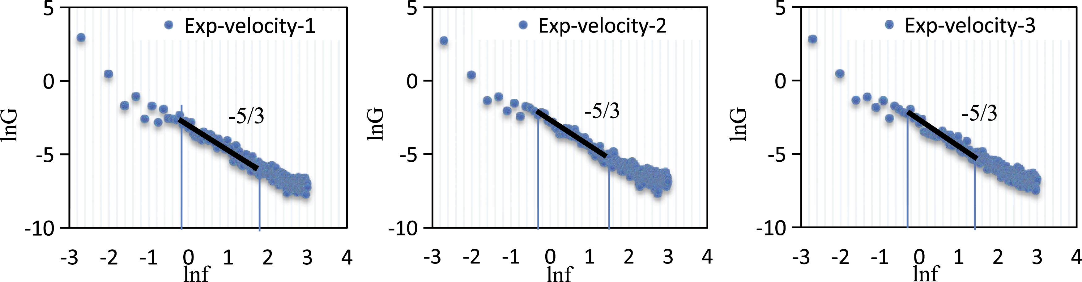

Grid sensitivity analysis and experimental validation

A grid sensitivity analysis was conducted before the simulation. Figure 7 shows the attenuation of carbon dioxide concentration difference of indoors and outdoors and the comparison of wind speed 2 m above the building roof. We found that when the number of grids was more than 6.06 million, the attenuation curves of indoor–outdoor concentration difference almost coincide with each other. It maintains a good consistency between calculated wind speeds based on 6.06 million gird and 9.80 million. The results show that the 6.06 million grids were sufficient for the pollutant distribution and the airflow simulation and can produce a relatively grid-insensitive result.

Figure 7.

Grid sensitivity analysis results: (a) attenuation of carbon dioxide concentration and (b) comparison of wind speeds 2 m above the building roof.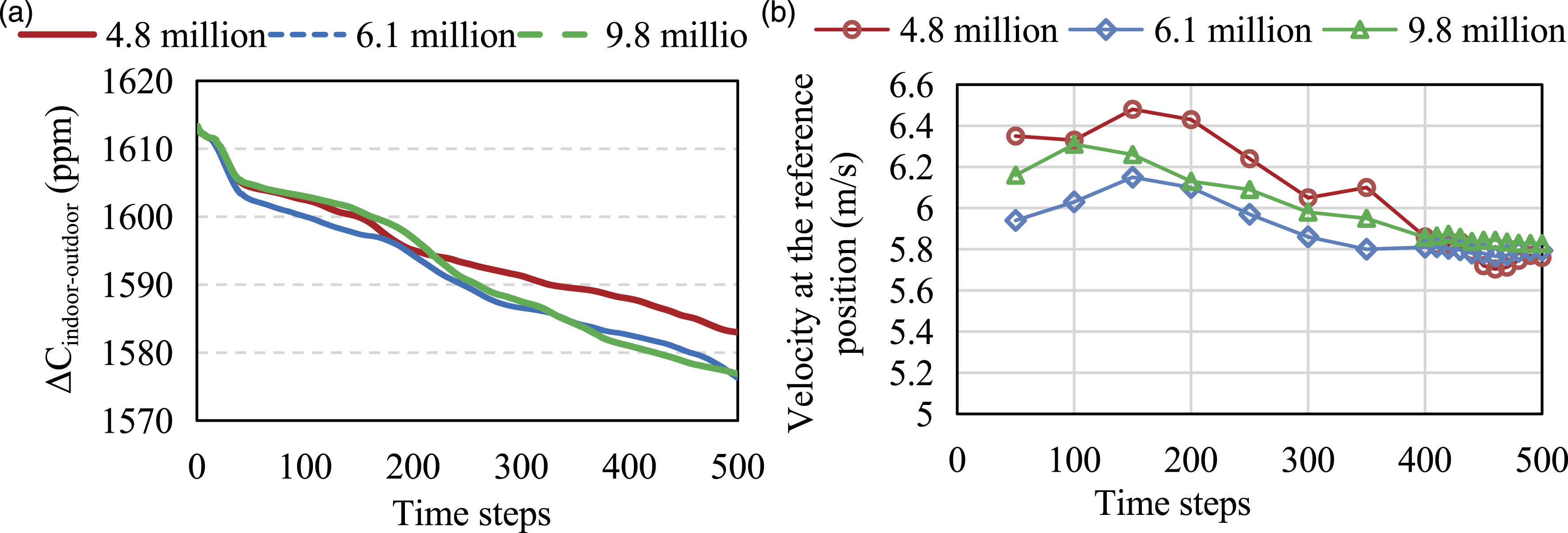

The Smagorinsky–Lilly model was used to simulate the airflow and contaminant transmission under single-sided natural ventilation in the building group as shown in Figure 2. Due to the high fluctuation characteristics of natural ventilation and the measurement frequency of the weather station, we compared the simulation results of the last 10 s of each minute with the measured average velocity. Figure 8 depicts the comparison of average velocity in the last 10 s per minute and the power spectrum of calculated and experimental results at sampling location Exp-1 as shown in Figure 1(b). The G is the power spectral density function and f is the frequency. The average error between the simulated average velocity and the experimental measurement was 38%. Although the error in wind velocity was not small, considering the unsteady fluctuation of natural ventilation, we believe the error was acceptable. The results in Figure 8(b) proved that the simulated energy spectrum was in good agreement with the experimental results.

Figure 8.

Comparison of calculated and experimental results: (a) average speeds per minute and (b) the power spectrum based on 5-minute wind speed series.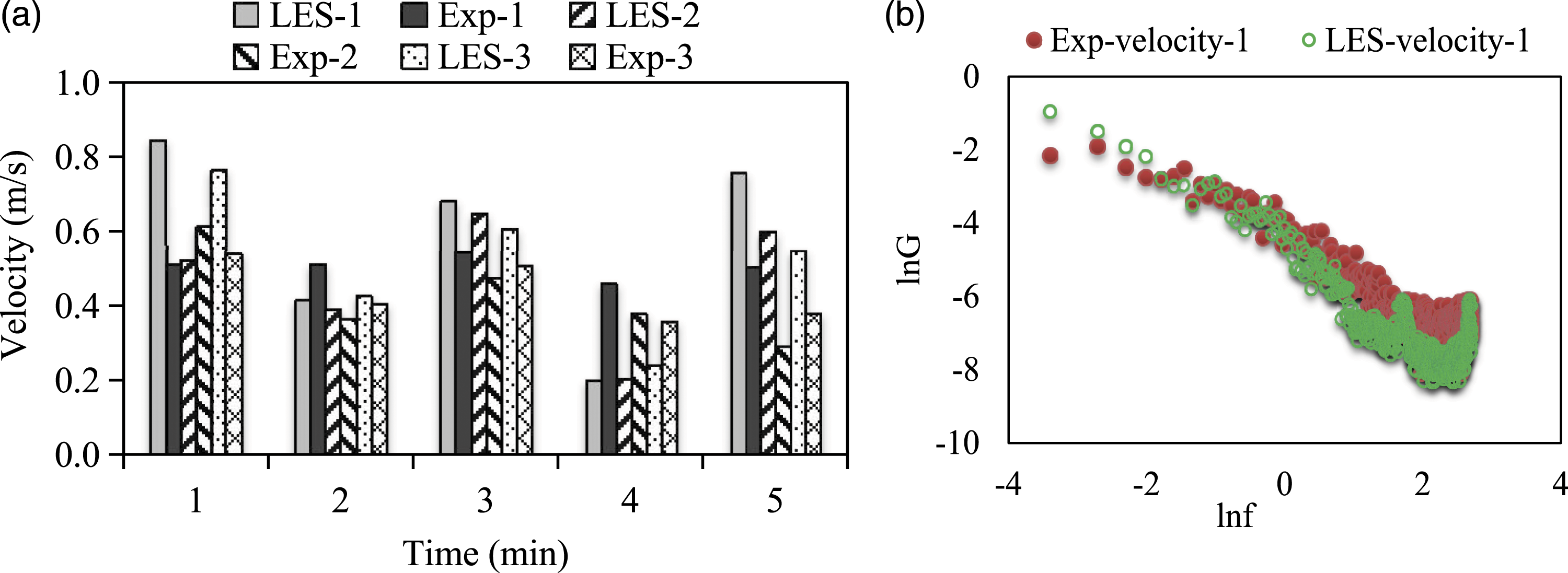

For the verification of pollutant diffusion, Figure 9 shows the attenuation of the indoor–outdoor CO₂ concentration difference (C_{indoor-outdoor}) with corresponding located experimental results. We used the 5-minute result of an experimental measurement for numerical simulation verification, and the attenuation time was calculated from the beginning of the 5-minute validation experiment. In Figure 9, LES calculation can clearly show the fluctuation of pollutant concentration, but the experimental results only showed a continuous decrease in the concentration. On the whole, the calculated result is in good agreement with the experimental data.

Figure 9.

Attenuation of indoor–outdoor CO₂ concentration difference (C_{indoor-outdoor}) with time.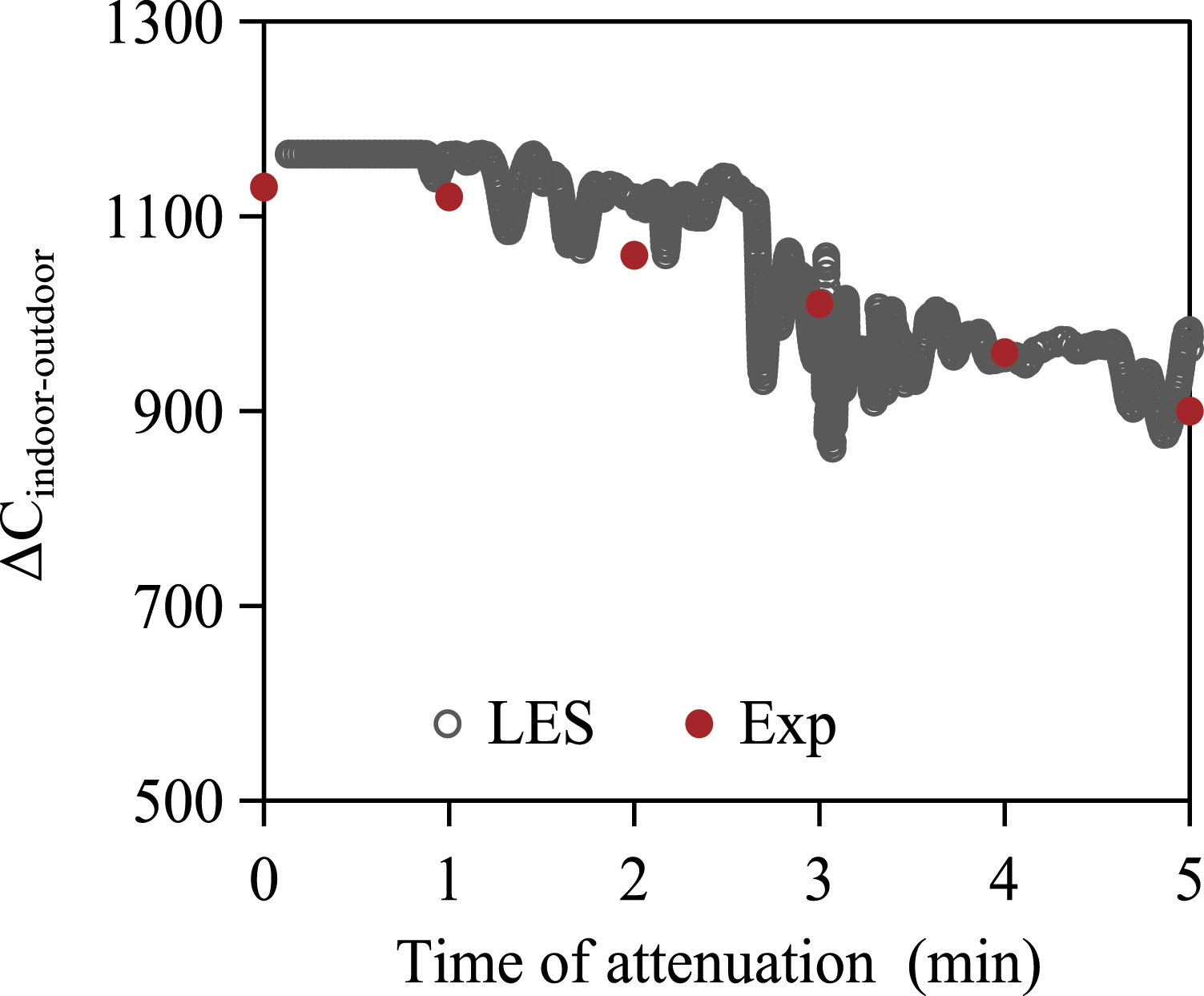

Instantaneous airflow and ventilation efficiency

Figure 10 displays the transient flow fields of the whole window as shown in Figure 1(b) at the end of every minute and the average velocity distribution vertical to the window (y direction). The incoming wind speeds in these 5 minutes in Figure 10 were 2.77 m/s, 2.01 m/s, 1.51 m/s, 2.27 m/s and 2.27 m/s, respectively. In the first minute, as portrayed in Figure 10(a), the airflow was outward on the left side of the window and inward on the right side. Because the incoming wind direction was westerly and parallel to the window, resulting in the air flow in and out in a left–right distribution, and the dividing line was irregular. After 2 min, with the decreased wind speed, the flow field changed to outward flow at the upper left corner and inward flow at the lower right corner. The dividing line was close to the diagonal of the window. With the further decrease in incoming wind speed, the air outflow area further moved up. The instantaneous flow field after 3 min exhibited outward airflow at the upper part of the window and inward airflow at the lower part, as shown in Figure 10(c). With the increase in the inlet wind speed, air flowed in from the upper part of the window and flowed out from the lower part after 4 min and 5 min. The variation in the wind speed had likely caused the variation in the air pressure at different positions on the window, which caused the changes in the entrance and exit areas. Due to the same inlet velocity between 4 min and 5 min, the airflow field at the window was relatively similar. Meanwhile, Figure 10(f) shows the average flow field in this 5 min. Generally, there was an outward flow at the upper part of the window and an inward flow at the lower part. However, the regions of inflow and outflow in the instantaneous flow field at the window varied with time, and the boundaries were all irregular. Therefore, it would not be reasonable to divide the window into half inflow and half outflow for the simulation of single-sided natural ventilation. The mean airflow field cannot show the instantaneous characteristics of flow with time in this period, and the instantaneous ventilation rate and its influence on indoor thermal comfort should not be ignored.

Figure 10.

Airflow field at the ventilated window with different entrance boundaries by LES: (a) 1 min, (b) 2 min, (c) 3 min, (d) 4 min, (e) 5 min and (f) mean velocity.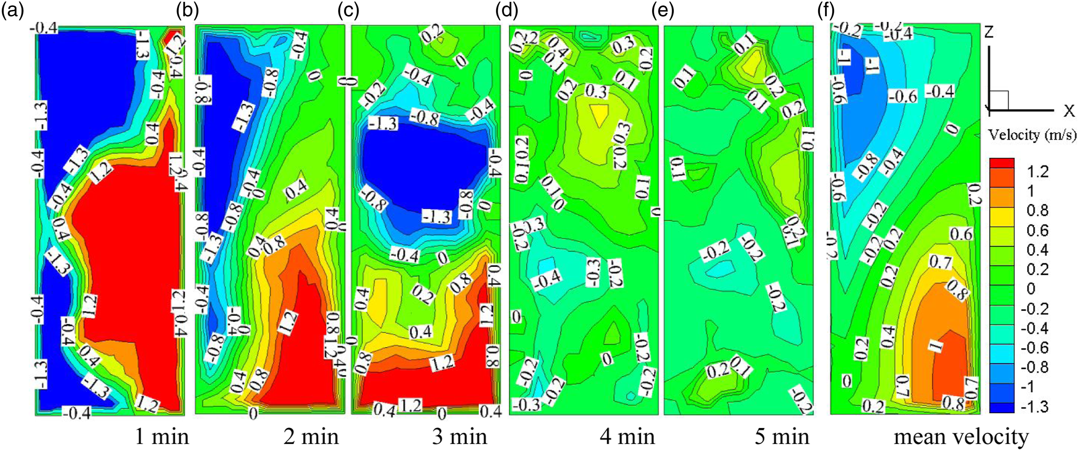

Since the inlet boundary condition changed once every 1 min, Figure 11 shows the transient airflow fields at different times with the same entrance velocity. As a whole, the air flowed in at the upper part of the window and flowed out at the lower part. Although the boundary conditions were unchanged, the airflow field at the window produced different distributions. Especially after the fourth and fifth minutes, the regions of airflow in and out were arranged in layers. The regions of air inflow changed at different times, which is not the typical up-down distribution as the average results. Large-eddy simulation can reproduce the airflow field at different times and reflect the influence of the airflow field at the previous time on the next moment, and provided more information of instantaneous airflow field.

Figure 11.

Instantaneous airflow field at different times with a same entrance velocity: (a) 4.17 min, (b) 4.33 min, (c) 4.5 min, (d) 4.67 min and (e) 4.83 min.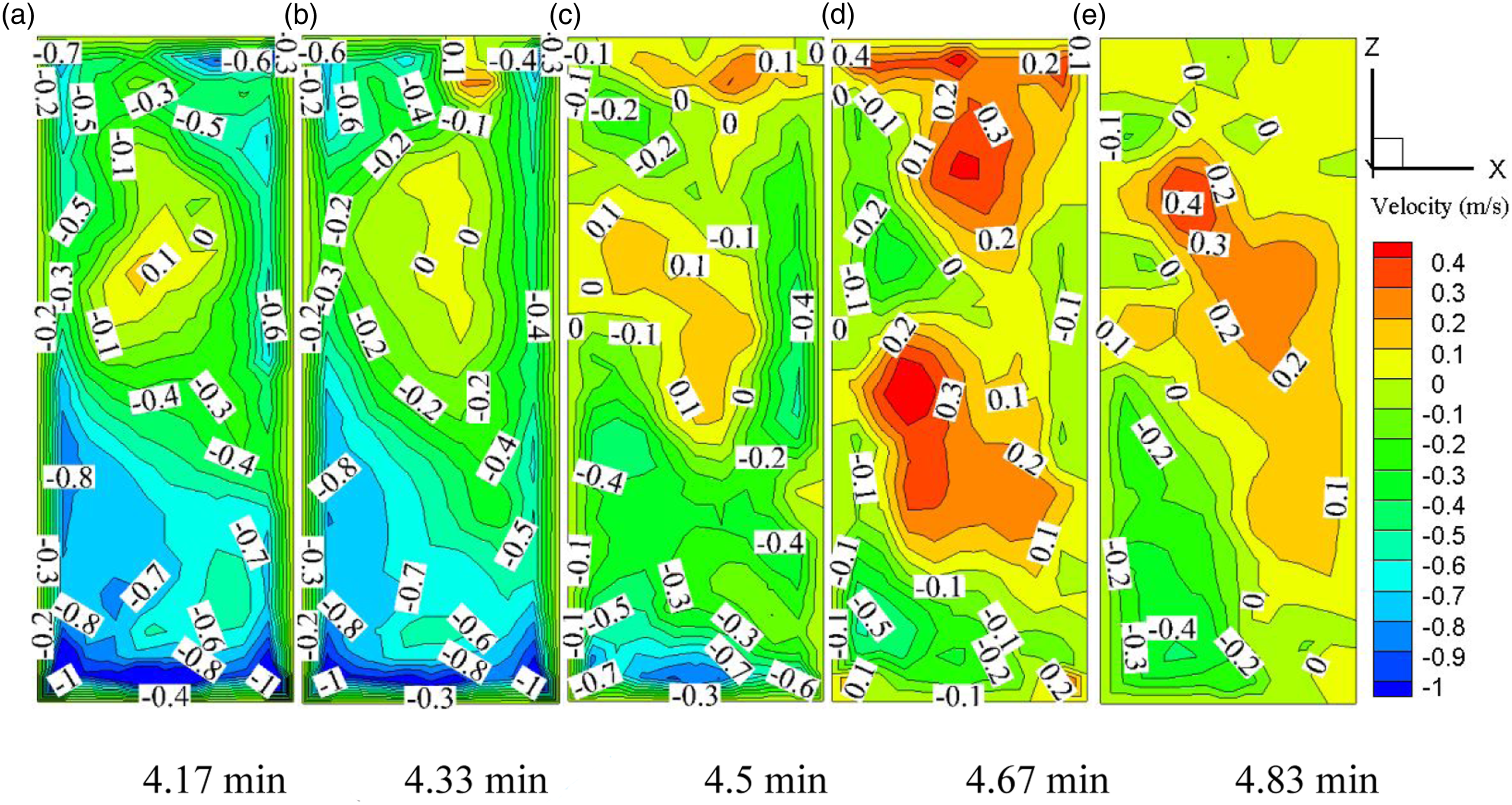

The inflow and outflow ventilation volume was obtained by counting the average wind speed of the inflow and outflow at the window and multiplying by the ventilation area. The inflow ventilation rate determined by the above simulation was 9.4 h⁻¹, and the measurement ventilation rate determined by the tracer gas attenuation method was 3.9 h⁻¹. The ventilation efficiency was 41.5%, the ventilation rate measured by the tracer gas method (effective ventilation rate) divided by the inflow ventilation rate at the window (ventilation rate into the room) by LES. The ventilation efficiency was so low because the incoming airflow was almost parallel to the window. The angle between the wind direction and the north direction was 275°, and the angle between the wind direction and the ventilation window was 5°.

Comparison of different inlet boundaries

Figure 12 shows the calculated air change rates by three inlet boundary setting methods. The results show that the air exchange rates of the ventilated room calculated by discrete wind speed entrance boundary (Disc) are very close to those measured by the tracer gas attenuation method, and the relative error is 11%. The difference between the calculated results with average velocity as inlet boundaries (Aver) and the experimental results is 29%. This may be because the average wind speed conceals the velocity fluctuation, which caused the overestimation in the pollutant results. Amongst the three inlet boundary setting methods, the calculation results with an average velocity superposition ±10% disturbance (Dist) are the most unsatisfactory, which may be because the ratio of the disturbance was unsuitable for use in all cases. The relative error between the experimental results and the simulated results is 64%. Therefore, the measured discrete wind speed is recommended as the inlet boundary for indoor and outdoor large-eddy simulation of real building groups. Because the required discrete wind speed series was not found in other literature, the simulation verification of other cases was not carried out. The results of our investigation provided a new idea for the boundary setting of large-eddy simulation of indoor and outdoor flow fields in a real environment.

Figure 12.

Comparison of air change rates calculated by different setting methods of the inlet boundary.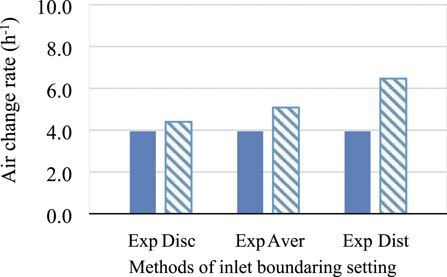

Conclusions

This investigation conducted site measurement of single-sided natural ventilation in urban building groups. A large-eddy simulation was used to simulate the indoor and outdoor airflow considering surrounding building groups, and the computed results were verified by the experiments. The following conclusions are drawn:

• The instantaneous airflow field measurement data of a single-sided natural ventilation window were obtained. The wind speed at the window of single-sided natural ventilation was highly unsteady, and the turbulence intensity in the middle part of the window was strong. According to the measured velocity series, the time step and grid scale of LES were calculated. The time scale in LES should be less than 0.17 s in this simulated condition, and the grid scale at the window needs to be between 0.7 mm and 95 mm.

• The Smagorinsky–Lilly model was verified to produce a good agreement with the experimental measurements on indoor and outdoor airflow fields by comparison of average air speeds, the power spectrum and indoor–outdoor CO₂ concentrations. Although the mean airflow at the window exhibited an obvious state of partial inflow and partial outflow under single-sided natural ventilation, the distribution of inflow and outflow was irregular. The natural ventilation efficiency was 42% with the incoming flow almost parallel to the window.

• The discrete wind speed at the inlet boundary is more suitable for the natural ventilation simulation of buildings in a real environment than the average wind speed boundary and the average wind speed superposition ±10% disturbance.

Footnotes

Author’ contribution

Wuxuan Pan: methodology, data duration and writing – original draft preparation. Zhengwei Long: methodology and funding acquisition. Chongfang Song: supervision and writing – reviewing. Yonggang Lei: supervision and writing – reviewing.

Declaration of conflicting interests

The author(s) declared no potential conflicts of interest with respect to the research, authorship, and/or publication of this article.

Funding

The author(s) disclosed receipt of the following financial support for the research, authorship, and/or publication of this article: This study was supported by the National Key R&D Program of the Ministry of Science and Technology, China, on ‘Green Buildings and Building Industrialization’ through Grant No. 2016YFC0700500) and the Applied Basic Research Programs of Shanxi Province (Grant No. 201901D111058; No. 202203021212246). This study was also supported by the science and technology innovation project of Shanxi Provincial Department of Education (No. 2021L079).

ORCID iDs

Wuxuan Pan

Zhengwei Long

References

Pourkiaei

Romain

. Scoping review of indoor air quality indexes: characterization and applications. Journal of Building Engineering 2023; 75: 106703.

Huang

ITS

Wong

Qian

. Role of air distribution in SARS transmission during the largest nosocomial outbreak in Hong Kong. Indoor Air 2010; 15(2): 83–95.

Yazarlou

Barzkar

. Louver and window position effect on cross-ventilation in a generic isolated building: a CFD approach. Indoor and Built Environment 2022; 31: 1511–1529.

Montgomery

Storey

Bartlett

. Comparison of the indoor air quality in an office operating with natural or mechanical ventilation using short-term intensive pollutant monitoring. Indoor and Built Environment 2014; 24(6): 777–787.

Qian

Zheng

. Ventilation control for airborne transmission of human exhaled bio-aerosols in buildings. Journal of Thoracic Disease 2018; 10(S9): S2295–S2304.

Huang

Feng

. Opening window issue of residential buildings in winter in north China: a case study in Shenyang. Energy and Buildings 2014; 84: 567–574.

Mak

Cui

. On-site measurements of ventilation performance and indoor air quality in naturally ventilated high-rise residential buildings in Hong Kong. Indoor and Built Environment 2015; 24: 214–224.

Aydin

Mirzaei

. Wind-driven ventilation improvement with plan typology alteration: a CFD case study of traditional Turkish architecture. Building Simulation 2017; 10(2): 239–254. DOI: 10.1007/s12273-016-0321-4.

Hooff

Blocken

Cao

. Mixing ventilation driven by two oppositely located supply jets with a time-periodic supply velocity: a numerical analysis using computational fluid dynamics. Indoor and Built Environment 2020; 29(4):603–620.

10.

Ricci

Burlando

Repetto

Blocken

. Simulation of urban boundary and canopy layer flows in port areas induced by different marine boundary layer inflow conditions. Science of The Total Environment 2019; 670: 876–892.

11.

Zhang

Chen

Wang

Liu

Mak

Fan

Hang

. Numerical evaluations of urban design technique to reduce vehicular personal intake fraction in deep street canyons. Science of the Total Environment 2018; 653: 968–994.

12.

Blocken

. LES over RANS in building simulation for outdoor and indoor applications: a foregone conclusion? Building Simulation 2018; 11: 821–870.

13.

Santiago

Borge

Martin

Paz

DDL

Martilli

Lumbreras

Sanchez

. Evaluation of a CFD-based approach to estimate pollutant distribution within a real urban canopy by means of passive samplers. Science of the Total Environment 2017; 576: 46–58.

14.

Zhang

Yin

Wang

O'Donovan

. Effect of cross-ventilation channel in classrooms with interior corridor estimated by computational fluid dynamics. Indoor and Built Environment 2021; 31: 1047–1065.

15.

Martins

Graca

GCD

. Validation of numerical simulation tools for wind-driven natural ventilation design. Building Simulation 2016; 9(001): 75–87.

16.

Chen

. Ventilation performance prediction for buildings: a method overview and recent applications. Building and Environment 2009; 44: 848–858.

17.

Shirzadi

Naghashzadegan

Mirzaei

. Improving the CFD modelling of cross-ventilation in highly-packed urban areas. Sustainable Cities and Society 2018; 37: 451–465.

18.

Blocken

Stathopoulos

Carmeliet

Hensen

JLM

. Application of computational fluid dynamics in building performance simulation for the outdoor environment: an overview. Journal of Building Performance Simulation 2011; 4: 157–184.

19.

Jiang

Alexander

Jenkins

Arthur

Chen

. Natural ventilation in buildings: measurement in a wind tunnel and numerical simulation with large eddy simulation. Journal of Wind Engineering and Industrial Aerodynamics 2003; 91(3): 331–353.

20.

van Hooff

Blocken

Tominaga

. On the accuracy of CFD simulations of cross-ventilation flows for a generic isolated building: comparison of RANS, LES and experiments. Building and Environment 2017; 114: 148–165.

21.

Farzad

Shahin

Payam

. Impact of opening shape on airflow and pollutant dispersion in a winddriven cross-ventilated model building: Large eddy simulation. Sustainable Cities and Society 2020; 61: 102196.

22.

Blocken

Sathopoulos

Saathoff

Wang

. Numerical evaluation of pollutant dispersion in the built environment: comparisons between models and experiments. Journal of Wind Engineering and Industrial Aerodynamics 2008; 96: 1817–1831.

23.

Tominaga

Stathopoulos

. Numerical simulation of dispersion around an isolated cubic building: model evaluation of RANS and LES. Building and Environment 2010; 45(10): 2231–2239.

24.

Wang

Yee

Lien

. Numerical study of dispersing pollutant clouds in a built-up environment. International Journal of Heat and Fluid Flow 2009; 30: 3–19.

25.

Jia

Kikumoto

. Construction of urban turbulence flow database ith wavelet-based compression: a study with large-eddy simulation of flow and dispersion in block-arrayed building group model. Journal of Wind Engineering and Industrial Aerodynamics 2021; 208: 104433.

26.

Camelli

Löhner

Hanna

. Dispersion patterns in a heterogeneous urban area. Mecnica Computacional 2005; 7: 1339–1354.

27.

Zhang

Lee

. Numerical simulation and in situ investigation of fine particle dispersion in an actual deep street canyon in Hong Kong. Indoor and Built Environment 2011; 20(2): 206–216.

28.

Gousseau

Blocken

Stathopoulos

van Heijst

GJF

. CFD simulation of near-field pollutant dispersion on a high-resolution grid: a case study by LES and RANS for a building group in downtown Montreal. Atmospheric Environment 2011; 45: 428–438.

29.

Mochida

Tominag

Kataok

Nozu

Shirasaw

. Cooperative project for CFD prediction of pedestrian wind environment in the Architectural Institute of Japan. Journal of Wind Engineering and Industrial Aerodynamics 2007; 95: 1551–1578.

30.

Liu

Pan

Zhao

Zhang

Cheng

Long

Chen

. Influence of surrounding buildings on wind flow around a building predicted by CFD simulations. Building and Environment 2018; 140: 1–10.

31.

Liu

Lee

. Evaluating the influence of transom window designs on natural ventilation in high-rise residential buildings in Hong Kong. Sustainable Cities and Society 2020; 62: 102406.

32.

Hanna

Brown

Camell

Chan

Coirier

Hansen

Huber

Kim

Reynolds

. Detailed simulations of atmospheric flow and dispersion in downtown manhattan: an application of five computational fluid dynamics models. Bulletin of the American Meteorological Society 2006; 87(12): 1713–1726.

33.

Jiang

Chen

. Effect of fluctuating wind direction on cross natural ventilation in buildings from large eddy simulation. Building and Environment 2002; 37: 379–386.

34.

Nozu

Kishida

Tamura

Okuda

Umakawa

. LES of Wind Turbulence and Heat Environment around Dense Tall Buildings, Proceedings of EACWE 5. Florence: Italy, 19 – 23 July 2009.

35.

Nozawa

Tamura

. Large eddy simulation of the flow around a low-rise building immersed in a rough-wall turbulent boundary layer. Journal of Wind Engineering and Industrial Aerodynamics 2002; 90(10): 1151–1162.

36.

Pan

Liu

Zhang

Cheng

Long

Chen

. A model for calculating single-sided natural ventilation rate in an urban residential apartment. Building and Environment 2019; 147: 372–381.

37.

Wang

Liu

Guo

Jiang

. Turbulence characterization of instantaneous airflow in an aisle of an aircraft cabin mockup. Building and Environment 2017; 116: 207–217.

38.

Werner

Wengle

. Large-eddy simulation of turbulent flow over a square rib in a channel. Berlin: Springer Berlin Heidelberg, 1989.

39.

Tan

H W

Kato

. Natural ventilation performance and mechanism on condition of fluctuating wind. Journal of Central South University (Science and Technology 2012; 43(6): 2424–2433.

40.

Buccolieri

Gromke

Sabatino

Ruck

. Aerodynamic effects of trees on pollutant concentration in street canyons. Science of the Total Environment 2009; 407(19): 5247–5256.

41.

Tominaga

Mochida

Yoshie

Kataoka

Nozu

Yoshikawa

Shirasawac

. AIJ guidelines for practical applications of CFD to pedestrian wind environment around buildings. Journal of Wind Engineering and Industrial Aerodynamics 2008; 96(10–11): 1749–1761.

42.

Smagorinsky

. General circulation experiments with the primitive equations: I. the basic experiment. Monthly Weather Review 1963; 91(3): 99–164.

43.

Chen

Zhao

. Some questions on dispersion of human exhaled droplets in ventilation room: answers from numerical investigation. Indoor Air 2010; 20: 95–111.

44.

Leng

Wang

Liu

. Sustainable design of courtyard environment: from the perspectives of airborne diseases control and human health. Sustainable Cities and Society 2020; 62: 102405.

Measurement and large-eddy simulation of single-sided natural ventilation in urban building groups

Abstract

Keywords

Introduction

Field measurement

Large-eddy simulation

Computational domain and grid

Boundary conditions

CFD model

Results and discussion

Measurement results

Grid sensitivity analysis and experimental validation

Instantaneous airflow and ventilation efficiency

Comparison of different inlet boundaries

Conclusions

Footnotes

Author’ contribution

Declaration of conflicting interests

Funding

ORCID iDs

References