Sage Journals: Discover world-class research

Abstract

Although the thermal environment of buildings with thermally complex building envelopes can be predicted, comprehensive guidelines are not available for designers to implement the thermal-environment analysis. Therefore, this study examines the application scope of advanced thermal-analysis methods from the designers’ perspective. The results of the simple model were consistent with the experimental values, with an error of approximately 0.5°C. The analytically determined convective heat-transfer-coefficient values were within 0.3–0.5°W・m²K, and the difference in the predicted values between the results of the simplified and detailed models was minor. The convective heat transfer coefficient calculated using the reference temperature defined at the dimensionless distance y+ was more accurate than that was obtained using the general energy simulation incorporating the boundary-layer theory. Although the simplified advection rate had a maximum error of approximately 150 m³/h, it was considered acceptable. The differences amongst the zones were less than 0.59°C, which is considered minor. The results obtained by using summer advection were sufficiently accurate. Furthermore, the dew-point temperature was used to evaluate the risk of dew condensation. Specifically, the results indicated that the introduction of outside air increased the risk of condensation on the floor.

Keywords

Heat transfer simulation convective heat transfer coefficient transfer flow coupled simulation design approach

Introduction

Several thermal-environment simulation tools for buildings, such as energy simulation (ES) and computational fluid dynamics (CFD) simulation, have been developed, and various functions have been added to these tools over the years. In recent years, analysis tools have been developed for heating, ventilation and air conditioning (HVAC) system design with low computational load,¹ thereby enabling high-precision calculations. In addition, ES coupled with equipment such as radiating panels can extend the application range of these tools.² Although CFD simulation is computationally expensive, it can fully resolve the analysis area, and it can determine the temperature and wind-velocity distribution characteristics in space. Therefore, this tool has numerous applications, including analyzing vehicle interiors,^3–6 and is widely used in the architectural field. Moreover, it is widely used in the medical field to analyze the human body.^7,8

However, as CFD involves long-term calculations for buildings with complex envelopes, the overall analysis cost is prohibitively high, even when using supercomputers. A coupled analysis of ES and CFD was proposed to address this problem, which was systematically reviewed by Zhai et al.^9,10 A recent study conducted a coupled CFD, daylight simulation and ES analysis with the aim of improving both thermal and visual comfort.^11–14 A constant-air-volume ventilation system with local radiators in each zone was compared with a full air volume system with demand-controlled ventilation. The reduction in total energy consumption for both systems was estimated to be approximately 80%.¹⁵ Indoor-side analysis methods considering the coupling of advection quantities between multiple zones and coupling with equipment models have also been investigated.^16,17 A CO₂ demand-controlled ventilation system based on ES and CFD coupling was used to study ventilation volume optimization using energy-recovery ventilators for office spaces.¹⁷ Furthermore, a method for the coupled analysis of ES and CFD that employed equipment models in conjunction with proportional integral derivative control was developed.¹⁸ As a representative example of a coupled analysis of a large space, the energy demand and indoor microclimate of an HVAC system, including humidity control, were determined. The air conditioning system was studied, and the energy reduction rate was calculated.¹⁹ Furthermore, a coupled ES and CFD analysis of the flow rate at the opening determined the extent of natural ventilation.²⁰ However, these advanced environmental simulation techniques yield results that are not consistent with design practice.

Particularly, in a previous study, the advection flow between zones was coupled for buildings²¹; however, the primary focus was on energy and comfort, and the results deviated from the basic design knowledge used in practice. Several coupled ES–CFD analyses for atrium spaces have been reported.^22,23 However, it is difficult to compare the methods used for the analysis of the coupled advection flow between zones with the current state of research. Kato et al.²⁴ used the contribution ratio of indoor climate (CRI) to analyze the indoor thermal environment based on superposition without advection quantities. Additionally, a coupled ES–CRI model was developed for unsteady analysis.²⁵ Yamamoto et al.²⁶ expressed the heat input to a space as the heat loss from the wall surface and heat resulting from the increased temperature of the space. Furthermore, they developed a coupled ES–CFD analysis method and confirmed the accuracy of radiation calculations performed using ES for the unsteady analysis of radiation panels.²³ Applying these methods in design practice is difficult because they are advanced and typically incompatible with the existing design methods. In addition, although these methods are simple and help achieve the same purpose, the analysis methods for the advection between zones differ.

Togari et al.²⁷ constructed a block model for the advection between zones to predict the upper-temperature distribution in large spaces and confirmed that the calculated and measured values were consistent. The block model has been updated over the years, and a model coupled with heat transfer from the room-side surface has been developed.²⁸ Moreover, a specific method has been proposed for adaptation to atriums.²⁹ Although these methods have been applied to large spaces, they have not been demonstrated in residential-scale buildings; in addition, the geometry is simple and theoretical. Therefore, the optimal approach would be to use CFD to calculate advection between zones. The theoretical background can be easily understood by coupling the advection between zones. Zhang et al.³⁰ performed a coupled ES–CFD analysis to study the influence of window surfaces as building envelopes. The results were consistent with those obtained using thermal environmental analysis methods applied to complex thermal geometries. Furthermore, a coupled ES–CFD analysis of urban city blocks, considering the microclimate, was performed to develop a practical method.³¹

The coupled ES–CFD analysis has been applied in architectural and urban environmental engineering to study the effect of heat removal by wind flow according to the building geometry in urban areas.³² A comprehensive review revealed that studies using this method remain limited, possibly because of the highly technical nature of research.³³ The number of buildings with complex envelopes, such as the Dancing House and the Elbphilharmonie and Laeiszhalle in Hamburg, has increased.^34,35 Therefore, a two-dimensional heat flow tool known as Hygrabe as well as a coupled heat transfer and CFD analysis method (hereinafter referred to as the thermal environment analysis method with thermally complex building envelopes (TEAM-TComBE)) have been developed for use in the design of such buildings.^36,37 For example, the ‘Capital Gate’, a 160-m-high building in the United Arab Emirates, recognized as the world’s tallest leaning building in the Guinness World Records, has a characteristic aspect that can be thermally analyzed using TEAM-TComBE.³⁸ In addition, TEAM-TComBE can analyze the thermal environment of Zaha Hadid’s work,³⁹ which won the first prize in an international design competition for the New National Stadium that is likely to host the Olympic Games in Japan. These structures have thermally complex curved-surface geometries, and TEAM-TComBE can perform a preliminary thermal analysis of these structures at the design stage.

The thermal environment of stadiums has previously been analyzed using various methods.^40,41 The coupled ES–CFD method has been used to analyze the thermal environment within a dome-shaped stadium. Recent research on creating near-future weather data⁴² and studying its impact on energy consumption in urban areas reported a 24.1% reduction in annual energy consumption. Further, a coupled ES–CFD analysis of urban microclimates reveals that buoyancy affects local temperatures.³²

Therefore, TEAM-TComBE, which was developed by Yamamoto et al.,³⁷ can have diverse range of applications, from urban ventilation to the analysis of building interiors. However, there remains a lack of fundamental knowledge for extending this coupled analysis method to design applications.

Specifically, the following research aspects remain unclear: (1) reducing the calculation load by simplifying the analysis model developed by Yamamoto et al.³⁷; (2) developing guidelines for analysis during design by clarifying the definition of the reference temperature of the convective heat transfer coefficient, h; (3) reducing the calculation load by handling advection volume between zones during the seasonal calculation based on an annual calculation; and (4) extending the application range of TEAM-TComBE according to the dew point temperature (t_dew)–based condensation risk assessment. TEAM-TComBE can be used to analyze thermally complex building envelopes with a small computational load; it can maintain a specific level of accuracy once the setting conditions are clarified. However, it cannot be easily used with a graphical user interface. Therefore, only engineers with experience in environmental simulation research can use TEAM-TComBE for design purposes. The present study attempted to address this limitation.

A study on the design process using CFD³⁷ has shown that the universal thermal climate index has been reduced by 0.1–0.6°C. Studies have been carried out on energetic optimization-calculation range from those on passive design to those on radiant cooling; however, they do not optimize the geometry from a design perspective.^43–46

This study was aimed at extending the TEAM-TComBE method reported by Yamamoto et al.³⁷ to develop a set of guidelines for use in the thermal design process of buildings. This study compared the results of accuracy verification and computational-load reduction to accumulate fundamental knowledge for a basic design using the TEAM-TComBE method. Subsequently, the factors considered during the design process and the allowable range of error were examined. Guidelines for usage in the design process were obtained rather than reducing the computational requirements associated with the method. However, because this study is based on accuracy verification, applied studies, such as urban ventilation, are outside its scope. Moreover, this study does not intend to explore the integration of TEAM-TComBE into the design process; instead, it provides detailed guidelines for using TEAM-TComBE in design, which would be beneficial because the number of buildings with thermally complex geometries is expected to increase. Furthermore, performing environmental simulations has been difficult for design architects. The most frequent users of environmental simulation are facility designers. Therefore, this study intends to serve as a reference and motivate the emergence of a new type of facility designer, that is, ‘environmentalists’, in addition to ‘architects’ and ‘structuralists’.

Methods

Unlike the TEAM-TComBE method used in this study, the ASHRAE standard describes a general ES modelling method.⁴⁷ However, the TEAM-TComBE method is more accurate than the conventional boundary layer theory method because y+ is used for defining the reference temperature, and a velocity scale based on shear stress is applied. Furthermore, this method includes the advection volume treatment and reference temperature for h (convective heat transfer coefficient). Therefore, this study focused on Hygrabe2D,³⁶ a two-dimensional heat-flow calculation tool for building envelopes. EnergyPlus and ESPr were not considered in this study.^48,49 In the coupled analysis, the advection between zones was calculated using CFD. In addition, a velocity scale based on shear stress was used to define h, and the coefficient accuracy was confirmed in a forced convection field.⁴¹ Yamamoto et al.⁵⁰ also confirmed the accuracy of natural convection fields.

The heat balance equation for the space is expressed in Equation (1). Equations (2) and (3) are used for calculating the h_wall for which a velocity scale based on shear stress is used in the calculation of heat flow. In addition, y+ is used for defining the reference temperature, which appropriately represents the temperature of the turbulent zone. In this study, the definition of the reference temperature was considered to verify the computational load reduction and obtain the guidelines for the use of TEAM-TComBE in design practice.

V_{o l} \bar{c} \bar{γ} \frac{d T_{i}}{d t} = \sum_{j = 1}^{J} S_{i, j} h_{i . j} (T_{i, j} - T_{i}) + V_{o} c γ (T_{o} - T_{i})

(1)

q_{w a l l} = \frac{ρ_{f} C_{P, f} u_{τ}}{T^{+}} (t_{w a l l} - t_{f l u i d})

(2)

h_{w a l l} = \frac{q_{w a l l}}{(t_{w a l l} - t_{f l u i d})}

(3)

where

C_{p}

is the specific heat of air [J/kg·K],

γ

is the specific gravity [kg/m³], T_i,j is the room temperature of the object element j [K],

\bar{c} \bar{γ}

is the apparent heat-to-volume ratio of a room, including furniture [J/m³·K], S_i,j is the room area of the object element j [m²], h_i,j is the room convective heat transfer coefficient of the object element j [W/m²·K], V_o is the amount of ventilation with outside air [m³/s], c

γ

is the specific heat of air volume [J/m³·K],

h_{w a l l}

is the heat transfer coefficient on wall [W/m²·K], q_wall is the heat flow [W/m² ],

ρ_{f}

is the density of the fluid [kg/m³ ], C_p,f is the specific heat capacity of the fluid [J/kg·K],

u_{τ}

is the velocity scale based on wall shear stress [m/s], t_wall is the temperature of the wall surface [K], t_fluid is the fluid temperature [K] and

T^{+}

is the dimensionless temperature [-].

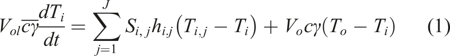
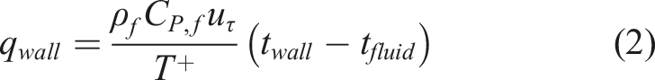
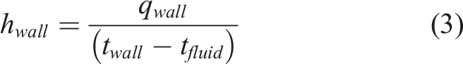
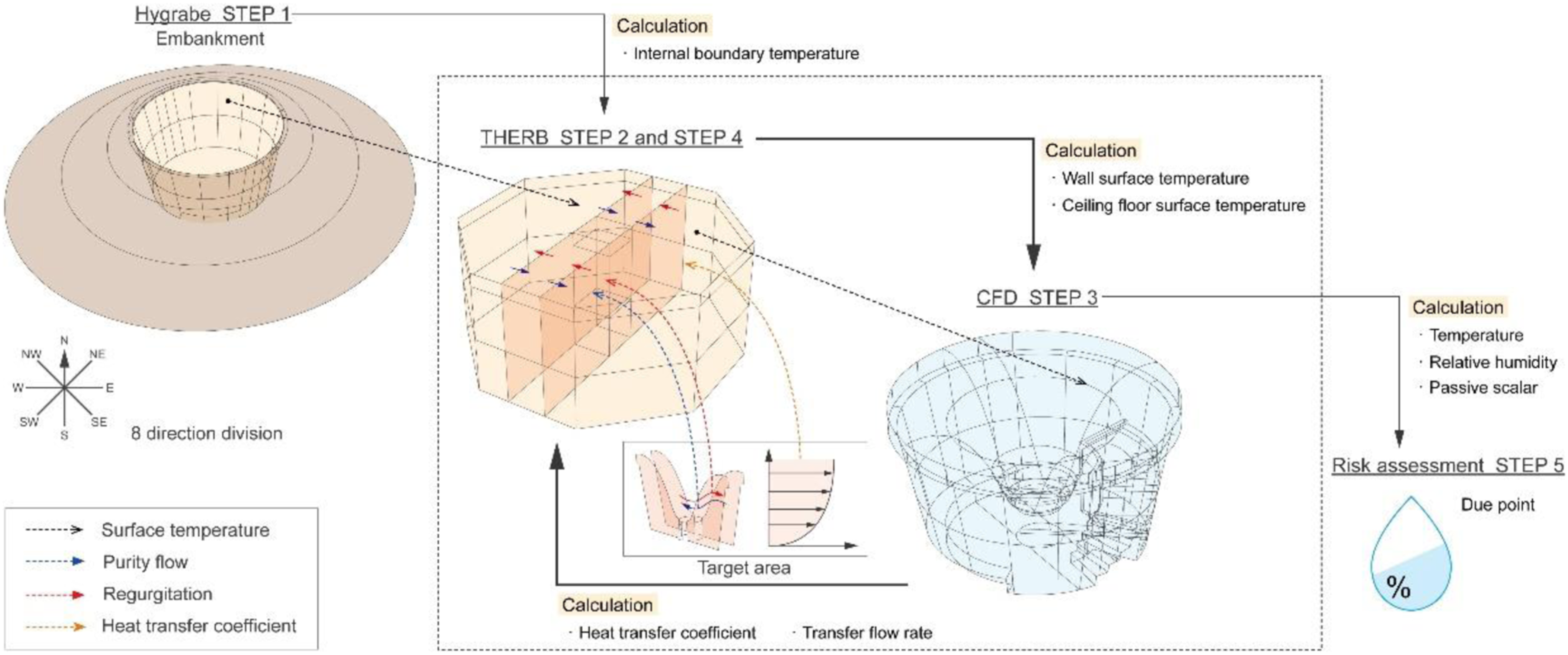
Figure 1 shows the flow diagram of the coupled simulation. In STEP 1, the building envelope was calculated in eight directions using Hygrabe2D. In STEP 2, the room temperature was calculated using THERB, and the surface temperature was calculated using Hygrabe2D and employed as a boundary condition. In STEP 3, the h and advection rate between zones were coupled to THERB using CFD. In STEP 4, the room temperature was again calculated using THERB. Finally, in STEP 5, t_dew was calculated using the temperature and relative humidity distribution obtained using CFD, and the condensation risk was evaluated.

Figure 1.

Flow diagram of the coupled process proposed by Yamamoto et al.³⁷

The analysis cost is considerably high if only CFD is used. In particular, the analysis cost of building envelopes with uneven surfaces, such as curved surfaces and building frame joints, is prohibitively high when only CFD is used for analysis. The cost can be substantially reduced by applying TEAM-TComBE. The two-dimensional heat flow calculation tool Hygrabe2D³⁶ is beneficial for reducing calculation costs. Moreover, in the coupled ES–CFD analysis, radiation calculations are performed in ES, which further reduces the CFD analysis cost. Furthermore, new possibilities could emerge if the analysis is performed by environmentalists experienced in environmental simulation.

The coupling flow in the study by Yamamoto et al.³⁷ is illustrated in Figure 2. The details of the convergence calculation are as follows. At time $t = 0$ , h was set to 4 W/m²K, and the THERB calculation was passed to CFD as a boundary condition. At $t = 1$ , the convective heat transfer and advection between zones analyzed by CFD at t = 0 were passed to THERB for the coupled analysis. At $t = 2$ , the calculated values of CFD were passed to THERB, similar to those at $t = 1$ , to check whether the final heat balance between THERB and CFD was achieved. This study compared the results of the second study for $t = 2$ . In addition, h was assumed to be constant because the daily room temperature did not substantially fluctuate owing to the high temperature of the fill.

Figure 2.

Comparison based on coupled flow of Hygrabe2D, THERB and CFD.³⁷

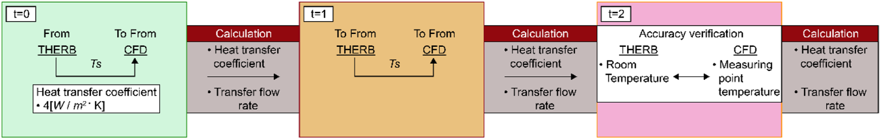
The ES calculations revealed no substantial variations in any zones, indicating that the fill was thermostatic. The following steps were used to determine the accuracy of the analysis:

(1) Confirm the accuracy of measurement points (CFD analysis).

(2) Confirm the thermal balance between THERB and CFD by comparing volume average temperatures.

(3) Compare the volume average temperatures in each CFD zone with the room temperatures in each THERB zone.³⁷

In this study, a specific test case, which was a modification of the one used by Yamamoto et al.,³⁷ was considered.

Figure 3 shows the factors considered in this study, a proposal for the environmentalists and the future vision for design utilization. The factors considered include (1) the possibility of reducing the calculation load by simplifying the analysis model, (2) presentation of the guidelines for the analysis during design by clarifying the definition of the reference temperature of h, (3) reducing the calculation load by handling the amount of advection between zones during seasonal calculations for annual calculations and (4) determining the risk of condensation based on t_dew.

Figure 3.

(a) Factors considered in this study and (b) the future vision for environmentalist advocacy and design use.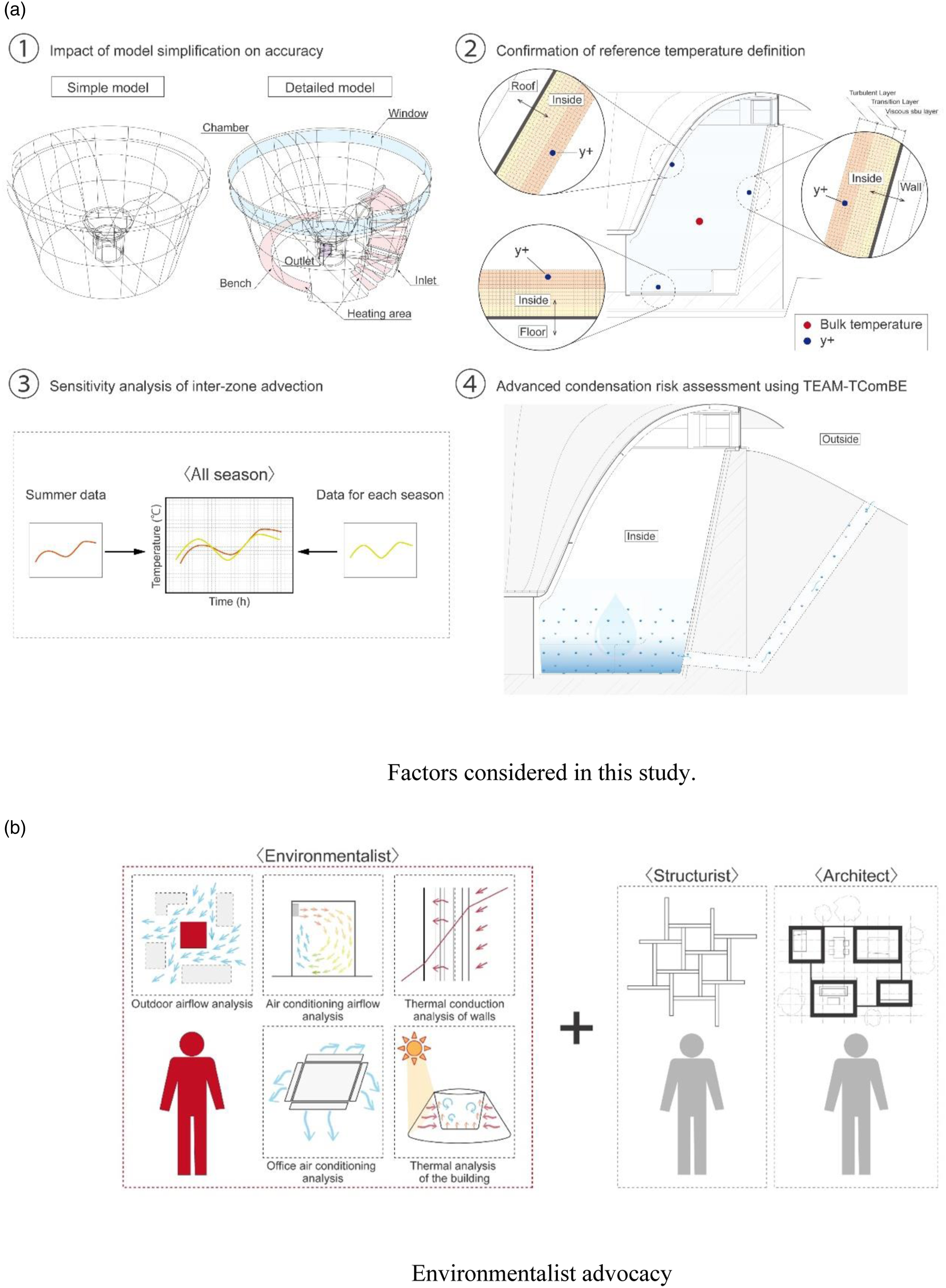

In addition, the design guidelines established in this study are expected to promote the design of environment-friendly homes. Kawashima et al.^51,52 used simple simulation tools for thermal, optical and other design needs in their design approach. In contrast, our design guidelines were limited to the coupled analysis of ES and CFD (TEAM-TComBE). Because guidelines or detailed studies do not exist, the results of this study can provide guidelines for step-by-step design utilization.

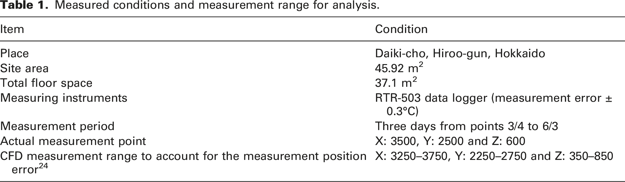
Figure 4 shows the measured points, plan and cross-sectional views of the building model. The building model is a spa with an embankment in Hokkaido, Japan, similar to that in the study conducted by Yamamoto et al.³⁷ The temperatures in the five zones did not differ substantially. Table 1 presents the actual measurement conditions and measurement range for verifying the CFD accuracy. Additionally, buildings that block solar radiation were not present in the vicinity of the model building. The outside air temperature was low during the measurement period, necessitating the use of heaters.³⁷ In addition, the measurement points used in the study were the same as those used by Yamamoto et al.³⁷ We compared the present study with that of Yamamoto et al.³⁷ The study is considered to be effective to a certain extent in terms of generalization; however, it needs further elaboration. The assumptions of the analytical model used in the present study are the same as those of Yamamoto et al.,³⁷ who verified these assumptions. Therefore, the analytical conditions were confirmed to ensure a certain level of accuracy. However, issues related to mesh independence are beyond the scope of this study. The number of meshes in this study was sufficient for safety.

Figure 4.

Plan (top) and cross-section (bottom) of the measured points and building model.³⁷

Table 1.

Measured conditions and measurement range for analysis.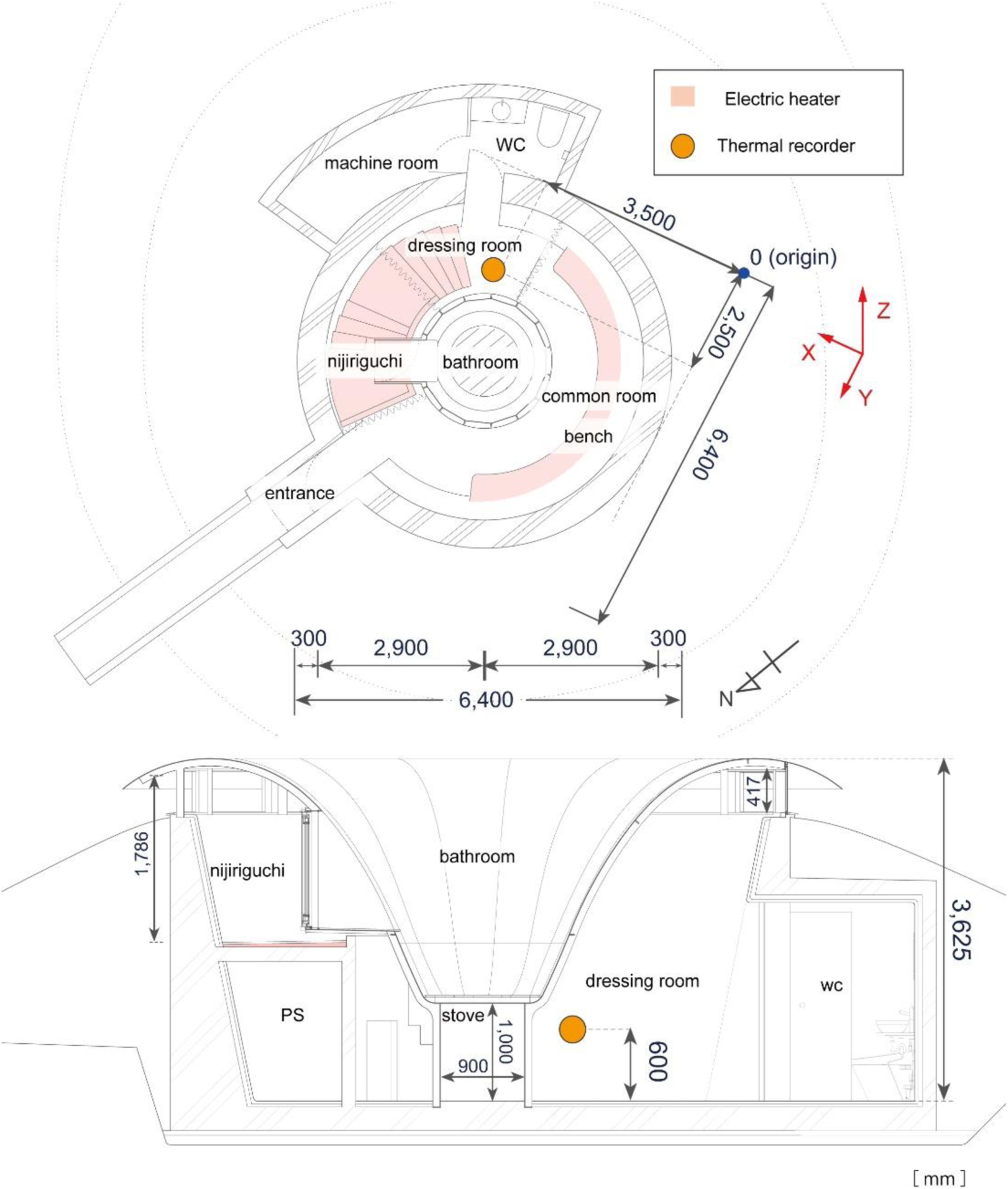

Item	Condition
Place	Daiki-cho, Hiroo-gun, Hokkaido
Site area	45.92 m²
Total floor space	37.1 m²
Measuring instruments	RTR-503 data logger (measurement error ± 0.3°C)
Measurement period	Three days from points 3/4 to 6/3
Actual measurement point	X: 3500, Y: 2500 and Z: 600
CFD measurement range to account for the measurement position error²⁴	X: 3250–3750, Y: 2250–2750 and Z: 350–850

Analysis model

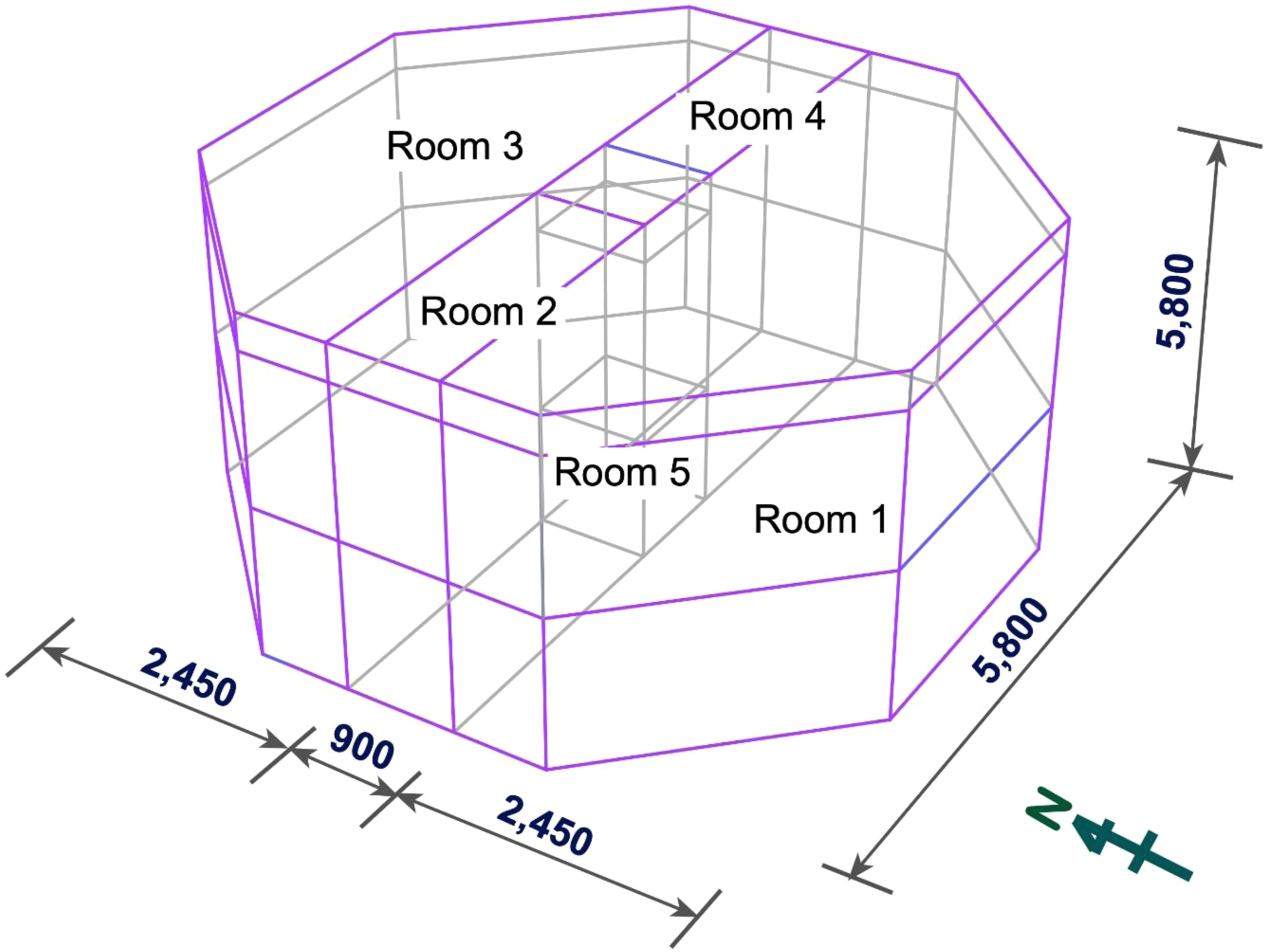
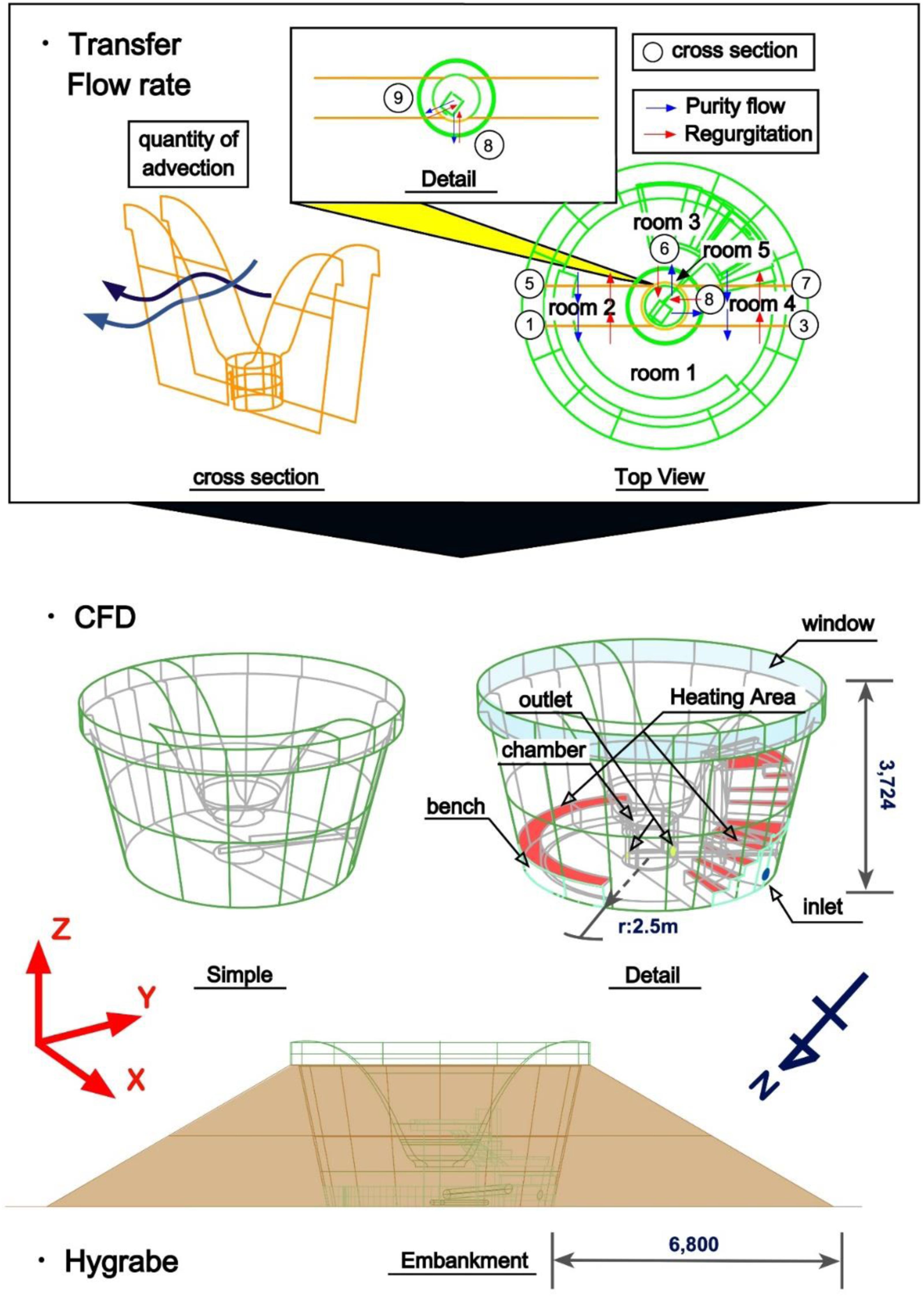
This section discusses the application of the proposed method for fill construction. The analytical model of THERB was divided into five zones with virtual walls inserted between them, as shown in Figure 5. The building envelope was analyzed using Hygrabe2D.³⁷ Figure 6 shows the CFD and Hygrabe analysis models and the virtual walls between zones. The detailed model includes the object to be analyzed, whereas the simple model does not contain furniture, stairs or benches. If a specific level of accuracy can be achieved using the simple model, it can serve as a benchmark for the designer. Furthermore, the detailed and simple models have slightly different spatial volumes, and the degree of analytical error is considered in each case. Moreover, simple models can be used when nonstationary analysis results are preferred over detailed modelling. The analysis load for the simple and detailed models depends on the number of meshes and computational power; however, a reduction of 2–3 h in computational load can be expected when a typical 14-core workstation is used. Notably, the reductions in the creation times of the CAD and THERB models can lead to a total reduction of at least 5–8 h in the computational load. The time estimates are not definite because they depend on the level of proficiency and machine specifications.

Figure 5.

Analysis model of THERB.³⁷

Figure 6.

CFD and Hygrabe analytical model.³⁷

The composition of the wall, which is consistent with that in the study by Yamamoto et al.,³⁷ is presented in Table 2. However, because of the high temperature of the fill, the strict insulation performance of the ZEH standard is not satisfied.⁵³ The analysis conditions for THERB and CFD are presented in Tables 3 and 4, respectively. We used Equation (4) to calculate the mesh resolution because calculating the spatial volume using Leaver’s formula is sufficient.⁵⁴ The mesh resolution of the simple and detailed models were 6.9 and 7.1 times higher than those of the model obtained using Leaver’s formula. Although the mesh resolution differed for the detailed and simple models because of the difference in spatial volume, the difference did not influence the analysis accuracy.

N = 44.4 \times 10^{3} \cdot V^{0.38},

(4)

where V is the room volume [m³] and N is the mesh resolution.

Table 2.

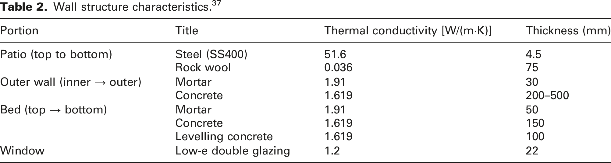
Wall structure characteristics.³⁷

Portion	Title	Thermal conductivity [W/(m·K)]	Thickness (mm)
Patio (top to bottom)	Steel (SS400)	51.6	4.5
Patio (top to bottom)	Rock wool	0.036	75
Outer wall (inner → outer)	Mortar	1.91	30
Outer wall (inner → outer)	Concrete	1.619	200–500
Bed (top → bottom)	Mortar	1.91	50
	Concrete	1.619	150
	Levelling concrete	1.619	100
Window	Low-e double glazing	1.2	22

Table 3.

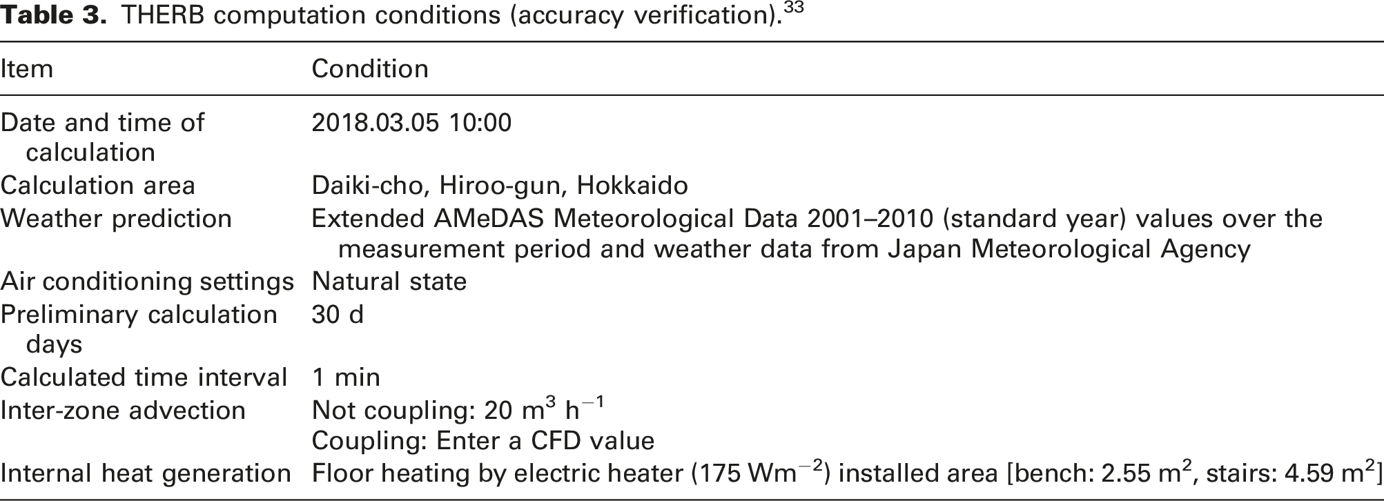
THERB computation conditions (accuracy verification).³³

Item	Condition
Date and time of calculation	2018.03.05 10:00
Calculation area	Daiki-cho, Hiroo-gun, Hokkaido
Weather prediction	Extended AMeDAS Meteorological Data 2001–2010 (standard year) values over the measurement period and weather data from Japan Meteorological Agency
Air conditioning settings	Natural state
Preliminary calculation days	30 d
Calculated time interval	1 min
Inter-zone advection	Not coupling: 20 m³ h⁻¹
Inter-zone advection	Coupling: Enter a CFD value
Internal heat generation	Floor heating by electric heater (175 Wm⁻²) installed area [bench: 2.55 m², stairs: 4.59 m²]

Table 4.

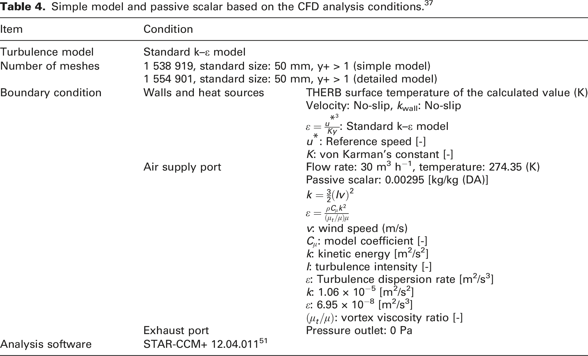
Simple model and passive scalar based on the CFD analysis conditions.³⁷

Item	Condition
Turbulence model	Standard k–ε model
Number of meshes	1 538 919, standard size: 50 mm, y+ > 1 (simple model)
Number of meshes	1 554 901, standard size: 50 mm, y+ > 1 (detailed model)
Boundary condition	Walls and heat sources	THERB surface temperature of the calculated value (K)
		Velocity: No-slip, k_wall: No-slip
		$ε = \frac{u^{*^{3}}}{K y}$ : Standard k–ε model
		$u^{*}$ : Reference speed [-]
		K: von Karman’s constant [-]
	Air supply port	Flow rate: 30 m³ h⁻¹, temperature: 274.35 (K)
		Passive scalar: 0.00295 [kg/kg (DA)]
		$k = \frac{3}{2} {(I v)}^{2}$
		$ε = \frac{ρ C_{μ} k^{2}}{(μ_{t} / μ) μ}$ v: wind speed (m/s)
		$C_{μ}$ : model coefficient [-] k: kinetic energy [m²/s²]
		I: turbulence intensity [-]
		$ε$ : Turbulence dispersion rate [m²/s³] k: 1.06 × 10⁻⁵ [m²/s²]
		ε: 6.95 × 10⁻⁸ [m²/s³] $(μ_{t} / μ)$ : vortex viscosity ratio [-]
	Exhaust port	Pressure outlet: 0 Pa
Analysis software	STAR-CCM+ 12.04.011⁵¹

The calculation conditions for Hygrabe2D are presented in Table 5. The analysis was based on four directions. Subsequently, the results of the seasonal introduction of advection between zones represented in the winter season were compared in Table 6.

Table 5.

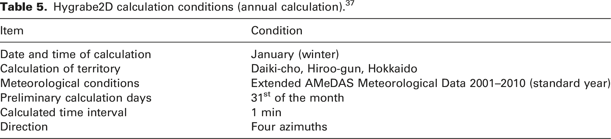
Hygrabe2D calculation conditions (annual calculation).³⁷

Item	Condition
Date and time of calculation	January (winter)
Calculation of territory	Daiki-cho, Hiroo-gun, Hokkaido
Meteorological conditions	Extended AMeDAS Meteorological Data 2001–2010 (standard year)
Preliminary calculation days	31^st of the month
Calculated time interval	1 min
Direction	Four azimuths

Table 6.

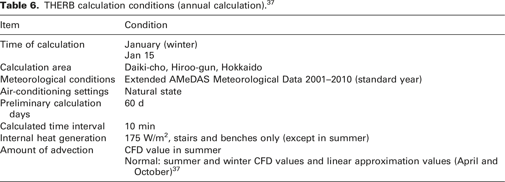
THERB calculation conditions (annual calculation).³⁷

Item	Condition
Time of calculation	January (winter)
Time of calculation	Jan 15
Calculation area	Daiki-cho, Hiroo-gun, Hokkaido
Meteorological conditions	Extended AMeDAS Meteorological Data 2001–2010 (standard year)
Air-conditioning settings	Natural state
Preliminary calculation days	60 d
Calculated time interval	10 min
Internal heat generation	175 W/m², stairs and benches only (except in summer)
Amount of advection	CFD value in summer
Amount of advection	Normal: summer and winter CFD values and linear approximation values (April and October)³⁷

Calculation results

Accuracy verification

Accuracy verification results of the second case

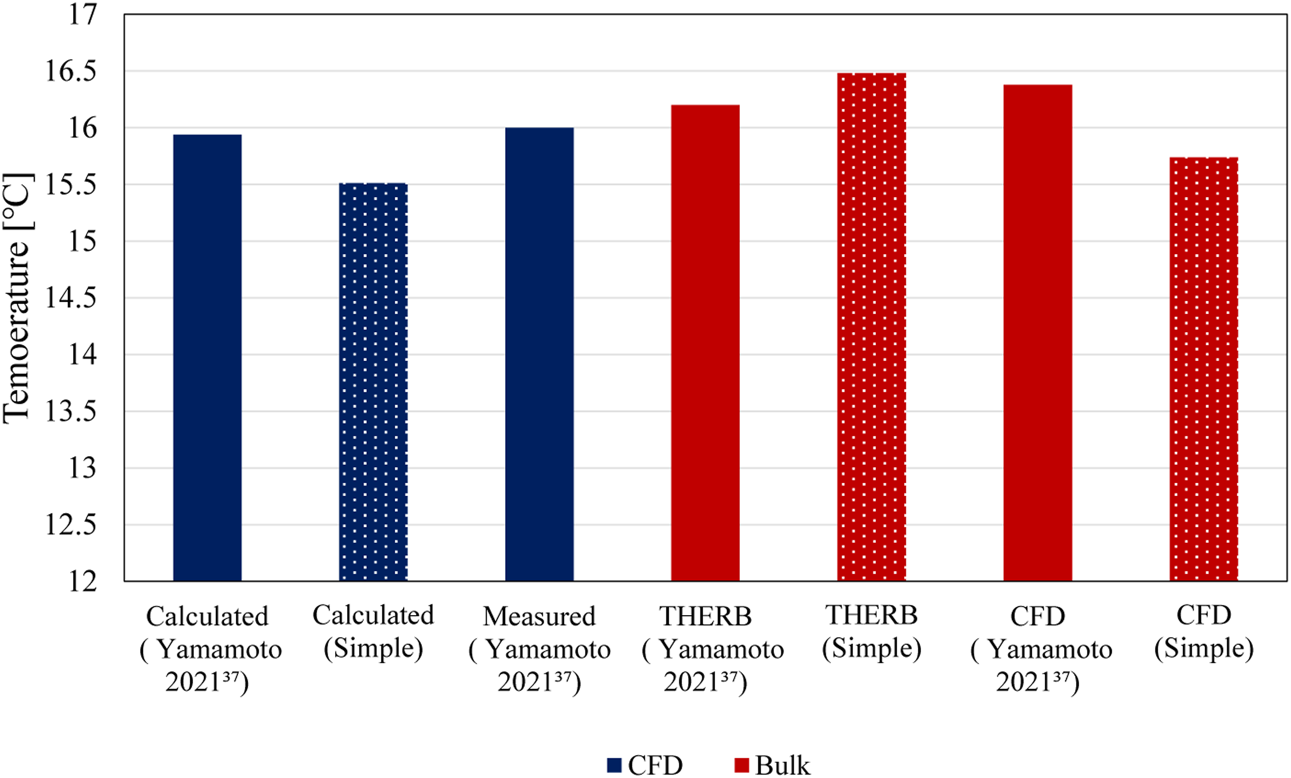
Figure 7 shows the results of the accuracy verification recorded at 10:00 a.m. on 5 March 2021. The temperature at the CFD measurement point (X: 3.25–3.75, Y: 2.25–2.75, Z: 0.35–0.85 unit [m]) was 15.51°C, and it was not tracked because of the imbalance between the volume of the space and the amount of heat supplied. Because the volumes of the simple and detailed models were larger than the volume of the wall in room 5, the amount of heat supplied was insufficient, thereby yielding a value slightly lower than the measured value. However, the error was only approximately 0.5°C, which was relatively small. In contrast, the volume average temperature obtained using THERB was 16.48°C, which was high. Although the thermal balance between THERB and CFD was not achieved because of their unequal volumes, the bulk temperature obtained using THERB was not considered a problem. The results of the unsteady analysis of the simple model adequately demonstrate the safety considerations.

Figure 7.

Accuracy test results performed at 10:00 a.m. on 5 March 2021 (comparison with previous studies).³⁷

Comparison of building and turbulence models

Figure 8 shows the reduction in the computational load obtained by simplifying the building model. Figure 8(b) shows the surface temperature obtained using THERB based on the calculation results of h using CFD. In the simple model, the overall value of h was in the range of 0.3–0.5 W/m²K. A slight difference from the detailed model was observed because of the change in the flow field caused by the simple model. The surface temperatures in rooms 3 and 4 that were obtained using the simple model were slightly higher than those obtained using the detailed model. Further, in room 5, the rate of temperature change was slightly higher in the simple model owing to the absence of walls. Therefore, the room temperature obtained using the simple model appeared to follow the temperature of each zone. However, as shown by Yamamoto et al.,³⁷ the zones in room 5 were either not divided into upper and lower zones to ensure that or the effect of air entering room 5 from the outside was already accounted for. Figure 8(c) shows the calculation results of the advection volume. The simple model yielded different results for advection because the stairs, benches and rooms were not modelled. In addition, the difference in the magnitude of the advection volume was insignificant. The maximum error of the simplified advection rate was approximately 150 m³/h. These results indicate that simplifying the model does not significantly affect the natural convection field when the boundary conditions are reasonable. Therefore, this finding can be included as a useful guideline in the design process.

Figure 8.

Results of calculation load reduction via building model simplification: (a) wall-surface temperature and h values of each room, (b) room temperature in each zone and (c) advection volume between zones.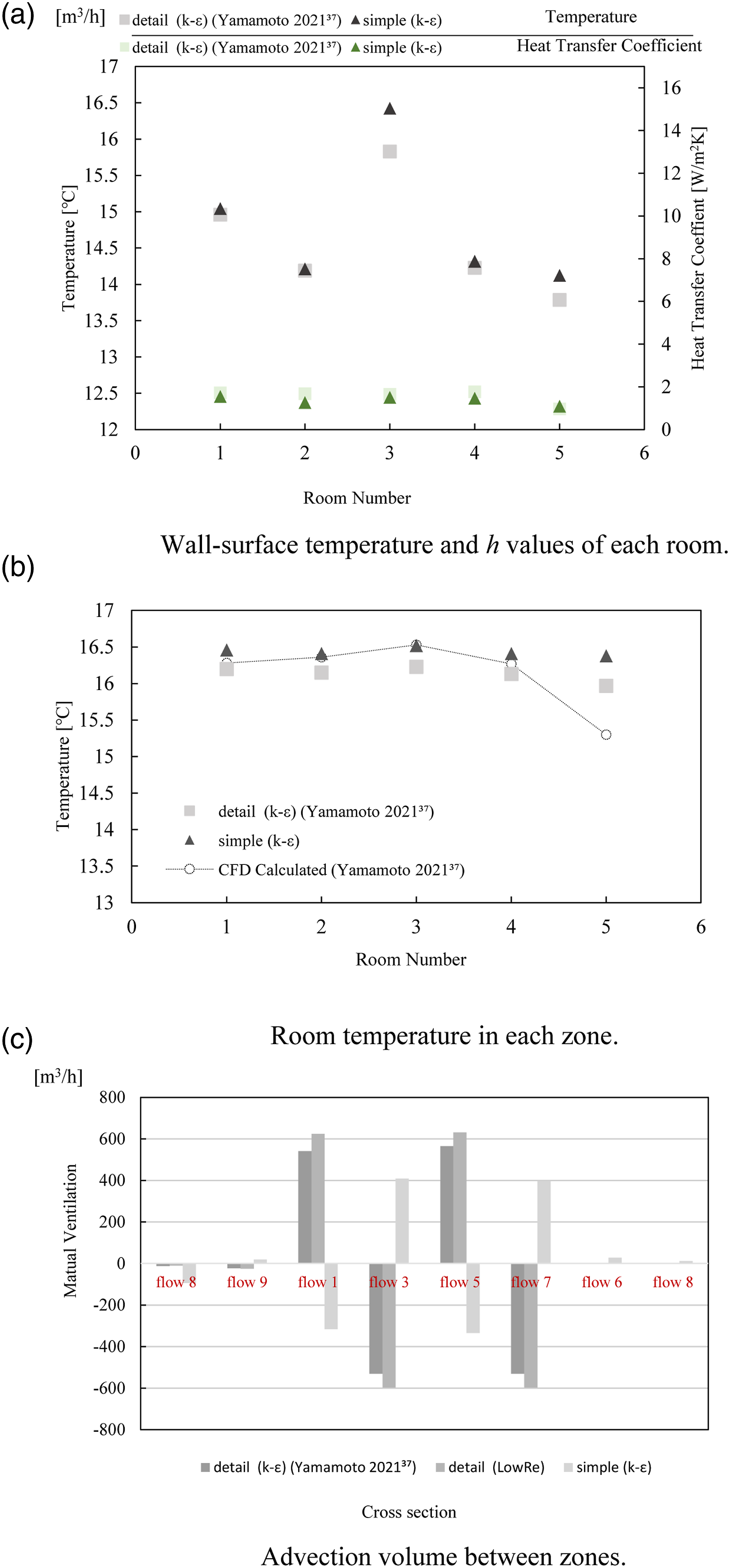

Using the space-volume average temperature as the reference temperature of the convective heat transfer coefficient

In Figure 9, the accuracy verification results and reference space temperature were compared. When the bulk temperature of the space was used as the reference temperature, the h value was obtained using Equations (5) and (6). The bulk temperature of the space referred to in the calculation of h was 16.38°C, that is, the volume average temperature. This study provides a guideline for defining the reference temperature of h, which would be helpful when using TEAM-TComBE in design, as defined by Equations (5) and (6).

q_{w a l l} = \frac{ρ_{f} {\cdot C}_{P, f} \cdot u_{τ}}{T^{+}} (t_{w a l l} - t_{c}),

(5)

h_{w a l l} = \frac{q_{w a l l}}{(t_{w a l l} - t_{c})} .

(6)

where t_c is the bulk temperature of the space [K].

Figure 9.

Comparison of the accuracy verification results with space temperature as the reference temperature: (a) comparison between h values obtained by Yamamoto et al.³⁷ and the bulk temperature used as the reference temperature and (b) comparison between the room temperature in each zone reported by Yamamoto et al.³⁷ and THERB.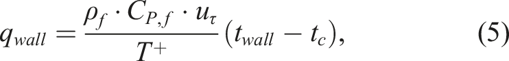

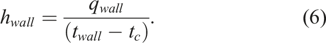
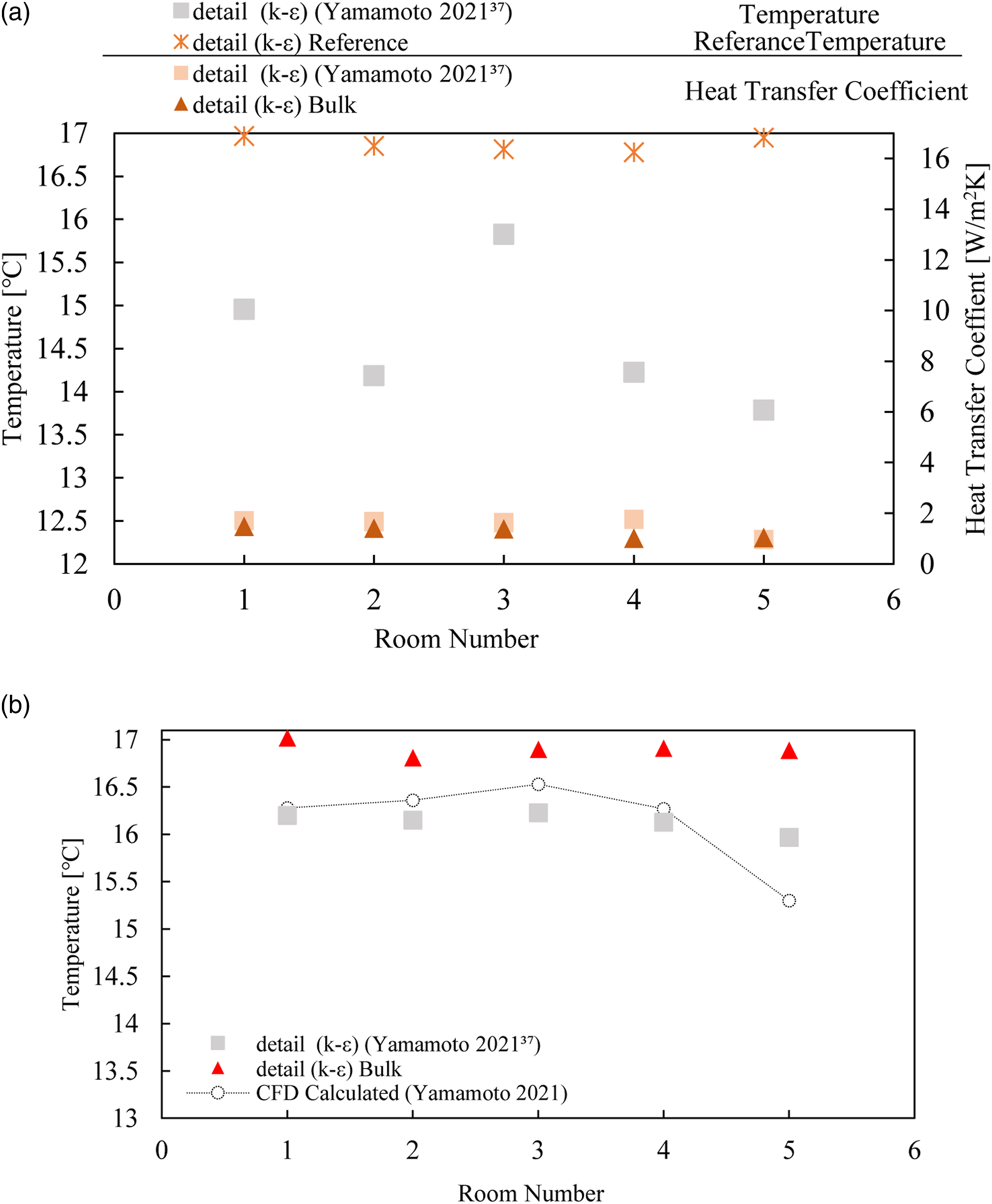
The calculated h in Figure 9(a) was lower than that was obtained by Yamamoto et al.³³ because a difference was not observed between the temperature near the wall and that in the space owing to the absence of advection by the air conditioner. Therefore, the high thermostability of the fill can be a factor.

The calculated room temperature for each zone of the THERB in Figure 9(b) was in the range of 16.81–17.02°C. Furthermore, the maximum value of h was 0.75 [W/m²K], which was low, suggesting that the temperature was high because the penetrating heat flow of the fill had negligible effect. In the natural convection field, the calculation of h using y+ to define the reference temperature was confirmed to be accurate in a laboratory with floor heating.¹⁶ Although the accuracy was confirmed using THERB, this method has not been compared with the calculation method in terms of the bulk temperature of the space. Notably, the detailed model yields the correct values, as shown in Figures 8(b) and 9(a), and the acceptable error threshold is approximately ±0.5°C, considering the results of the simple model. A large difference in spatial temperature results was obtained using only the bulk temperature as the reference temperature, indicating that ES used in the study is more accurate than the general ES that incorporates the boundary-layer theory with the bulk temperature as the reference temperature. These data are beneficial for using ES in the design stage.

Annual room-temperature calculation

Figure 10 shows the calculation results of the advection rate between the zones. The maximum value was 500 m³/h, which is not large. During the middle period, the median value was dependent on the summer advection rate and was the same as that in winter. The maximum value during winter was 51.7 m³/h, which was extremely low because the room temperature in the natural state influenced this value. Therefore, the environmental conditions in winter are not conducive to the generation of buoyancy.

Figure 10.

Calculation results of advection volume.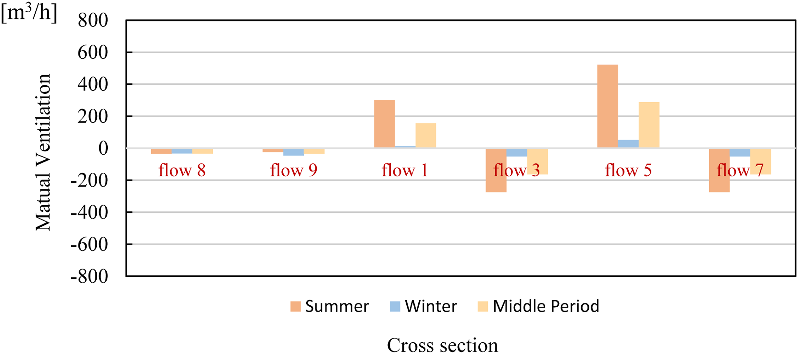

Figure 11 shows the results of the coupled analysis when summer advection was used in the intermediate months of April and October and in winter in January. The calculation results confirmed that almost no change occurred in the case where summer advection was used for the intermediate periods of April and October. However, the analysis results for the winter season indicated a maximum difference of 0.59°C at 12:00 in room 1, which was attributed to the large difference in the amount of advection between the zones. Consequently, to follow the room temperature of each zone with certainty, the calculation for each season should be performed. However, because the maximum difference is only 0.59°C, one season can be used as a representative season. This assumption yields an acceptable error for design purposes. Thus, the analysis load of CFD can be significantly reduced. Moreover, these considerations assumed that the design is safe.

Figure 11.

Comparison between the results of the coupled analysis of summer advection and the advection in each season: (a) room 1: Room-temperature change over time, (b) room 2: Room-temperature change over time, (c) room 3: Room-temperature change over time, (d) room 4: Room-temperature change over time and (e) room 5: Room-temperature change over time.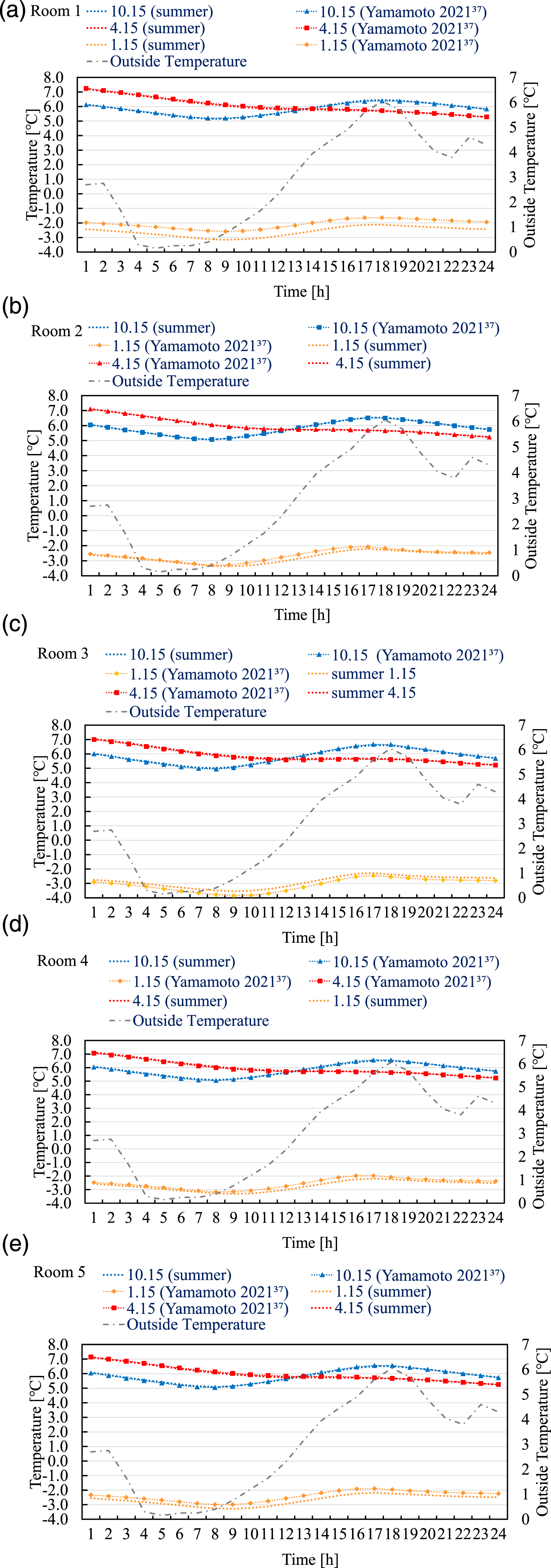

Condensation risk assessment

Hokkaido is located in a region that experiences snowfall. Therefore, condensation risk evaluation is a necessary consideration for the design guidelines. Because the condensation risk according to t_dew has not yet been determined using the coupled ES–CFD analysis, the approach used in the study can provide data that can be used as a guideline in the design process. Details of the cross-section of the condensation risk assessment from the origin, X: 2.9 m, Y: 2.9 m and Z: 1.77 m, are represented in Figure 12. The normal direction was set as X: −0.63 m, Y: 0.867 m and Z: 0.0 m and defined by a vector connecting this point with the origin of the selected coordinate system. Furthermore, the cross-section was selected to show the humidity inflow from the outdoor air inlet.

Figure 12.

Cross-section used in the condensation risk assessment study.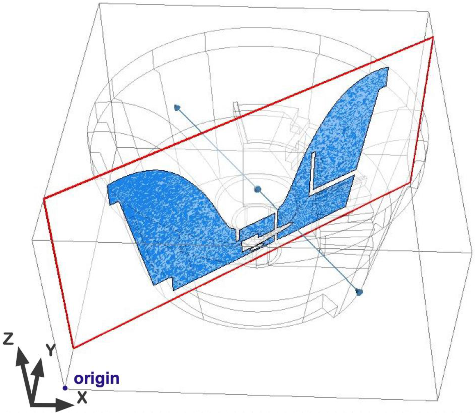

To determine t_dew, the saturated vapour pressure was calculated using Equation (7).

P_{w s} = A \cdot 10^{(\frac{m \cdot T}{T + T_{n}})}

(7)

Assuming that the relative humidity in the building is known, the vapour pressure is expressed using Equation (8). Further, t_dew is expressed using Equation (9).

P_{w} = P_{w s} \cdot R H / 100

(8)

t_{d e w} = \frac{T_{n}}{[\frac{m}{10 \log (\frac{P_{w}}{A})} - 1]},

(9)

where the constants are A = 6.116441 g/m³, m = 7.591386 g/mol and T_n = 240.7263 [K],

R H

: Relative humidity [%], T: Absolute temperature [K],

P_{w s}

: Saturation vapour pressure [hPa], t_dew is dew point temperature [K] and the vapour pressure P_w [hPa] is in the range of values corresponding to 20–50°C.

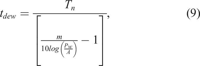
Figure 13 shows the analysis results of the CFD distribution characteristics related to t_dew. The condensation risk assessment revealed that the risk of condensation near the floor was high because of the incorrect selection of the air conditioning system. Countermeasures could have been implemented if this condensation risk assessment had been conducted in advance.

Figure 13.

Analysis results of the CFD distribution characteristics related to t_dew: (a) temperature distribution, (b) wind velocity distribution, (c) relative humidity distribution and (d) t_dew distribution.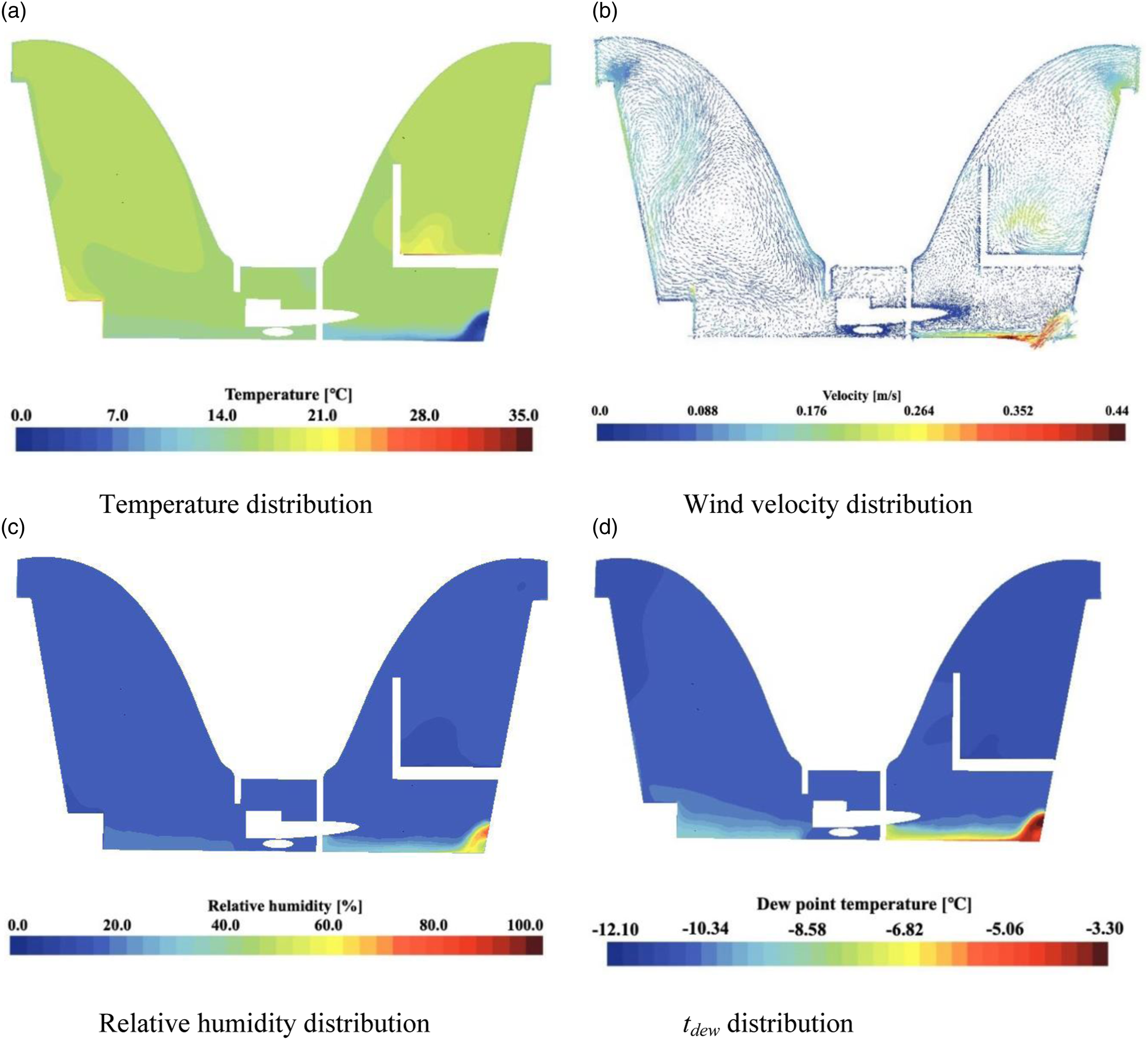

The maximum wind-velocity distribution observed in Figure 13(b) was approximately 0.44 m/s. The draught at the foot of the air conditioner is concerning. However, the temperature distribution in Figure 13(a) indicates that the temperature fell locally only near the inlet, and the results in Figures 13(c) and (d) demonstrate that the relative humidity was high only near the inlet. Moreover, the risk of condensation was high near the inlet. The risk of condensation cannot be fully evaluated based only on temperature, wind velocity and humidity. Therefore, depending on environmental conditions, evaluation by dew-point temperature is significant because of the correlation between temperature and dew-point temperature. Because the purpose of this study is to present a model case for condensation risk assessment, detailed analysis is beyond the scope of this work.

Limitations and scope for future work

In this study, various investigations were conducted to demonstrate the prospects of TEAM-TComBE. The limitations and the corresponding scope for future work are as follows:

(1) This study is limited to one analytical model; therefore, it is not fully generalizable but useful within a certain range. Additionally, the governing equations should be separately obtained because the dew-point-temperature study assumes a passive scalar. However, because this study primarily aimed to present possibilities for design, this aspect was beyond the scope of this work.

(2) Although previous studies have broadened possibilities, the model and analytical conditions – specifically, the forced convection fields such as air-conditioner operation – have not been studied in combination. Future development may include the adaptation of TEAM-TComBE in forced convection fields such as air conditioning. Additionally, TEAM-TComBE can be extended to complex flow fields, such as those in which radiant panels and air conditioners are used in combination.

(3) The reference temperature for the convective heat transfer coefficient is defined at y+. In general-purpose CFD software, defining the reference temperature of the convective heat transfer coefficient at y+ is difficult. However, this can be implemented in advanced CFD software, and used by expert CFD engineers. Therefore, to enhance the applicability of TEAM-TComBE, the software can be upgraded to easily estimate the convective heat transfer coefficient from flow fields that vary with geometry and conditions using CFD software mainly used for design purposes.

(4) TEAM-TComBE does not evaluate comfort. Therefore, for future work, we will consider using TEAM-TComBE to evaluate comfort. Furthermore, we will develop a coupled analysis model that includes calculations concerning the characteristics of installed facilities and equipment to evaluate energy efficiency. This coupled analysis model can analyze various building types: residential, office and high-rise buildings; the building is assumed to have a thermally complex shape.

(5) The study requires further investigation into the advection between zones in the forced convection field due to the installation of equipment and devices. Therefore, for future work, the first step is to experimentally measure inter-zone advection and room temperature. The second step is to verify the accuracy of the inter-zonal advection and confirm that the room temperature agrees with the experimental values. This step requires measuring several parameters to ensure an appropriate representation of the experimental values. In the third step, the first and second steps are reviewed by changing the parameters of the experiment to assess generality.

(6) The limits of inter-zonal advection coupling should be confirmed. Experiments will be conducted on a simple model using TEAM-TComBE, and the results will be evaluated via sensitivity analysis using various parameters (model geometry, space temperature, building envelope geometry, etc.). Depending on the experimental and analytical results, TEAM-TComBE can be extended to analyze spaces using methods other than coupled inter-zonal advection.

(7) The method used in this study to indicate reference temperatures for convective heat transfer coefficients is complex, and a simpler method can be developed. Specifically, artificial intelligence (AI) can be used on a large amount of experimental data to accurately capture reference temperatures for turbulent regions, or the accuracy can be improved using a semi-experimental formula with new dimensionless distances as improved indicators for various geometries. In either case, a large amount of experimental data and machine learning by AI would be effective for implementation. Several variables should be considered because indices such as surface roughness will have a significant influence.

In general, the scope of application of TEAM-TComBE is wide and can be applied for continuous analysis, from urban environments to interior design. In particular, TEAM-TComBE is expected to be a powerful computational tool for analyzing the thermal environment of double-skinned and curved exterior skin based on the results of urban CFD analysis. However, TEAM-TComBE has not yet been coupled with urban CFD analysis. In the future, TEAM-TComBE will be applied to buildings with thermally complex geometries in urban districts. Moreover, the CFD analysis of urban districts will be upgraded to a comprehensive analysis method that would reflect the effects of airflow on the outdoor side, which would be extended to a thermal environment analysis calculation tool that adds the value of a ‘breathing’ building envelope and other techniques. Hygrabe can be modified to consider heat transfer in porous regions. Specifically, this method will be extended based on two-dimensional fluid analysis for next-generation air conditioning systems.

Conclusions

This study investigated the possibility of reducing the computational load using TEAM-TComBE for practical use. In addition, the condensation risk according to t_dew was evaluated using CFD analysis to determine the application range of TEAM-TComBE. The following findings were obtained:

• The study was conducted to ascertain the effect of the TEAM-TComBE method on the analysis of a thermal environment. Therefore, even if an insignificant influence was observed, it was considered beneficial as a new finding. First, the calculation results of h values were not severely affected unless the reference temperature was changed. The reference temperature of h should be defined at y+ for design applications. In addition, the advection between zones did not substantially affect the calculation results, even during the summer season. Therefore, the data from the summer season should be used as a reference in the design phase in terms of analysis load.

• In the analysis of the thermal environment, the h value and the amount of advection between zones must be regulated. This study obtained the fundamental data for constructing these design guidelines. Further, the detailed settings often overlooked during the design process were clarified, which is the first step towards combining design practice and advanced thermal environment simulation.

• In the design process, assumptions regarding annual calculations and the thermal insulation performance were made. Several conditions need to be considered for such a study, and the design is expected to be sufficient in terms of analysis accuracy.

The guidelines obtained in this study are as follows:

(1) y+ should be used to define the reference temperature when calculating h.

(2) Although the results depend on the space volume, simplifying the CFD model does not affect the accuracy of the unsteady analysis.

(3) No significant difference was observed amongst advection values in zones, although advection coupling is representative of a single season such as summer.

(4) The TEAM-TComBE method can evaluate condensation risk even in complex-shaped envelopes. Specifically, in cold regions, it is necessary to evaluate condensation risk at the design stage.

Footnotes

Declaration of conflicting interests

The author(s) declared no potential conflicts of interest with respect to the research, authorship, and/or publication of this article.

Funding

The author(s) received no financial support for the research, authorship, and/or publication of this article.

ORCID iD

Tatsuhiro Yamamoto

References

The BEST Program . ® (BEST: building energy simulation tool), https://www.ibec.or.jp/best/index.html (accessed 27 May 2022).

Strand

Baumgartner

. Modeling radiant heating and cooling systems: integration with a whole-building simulation program. Energy Build 2005; 37: 389–397.

Chiang

W-H

Wang

C-Y

Huang

J-S

. Evaluation of cooling ceiling and mechanical ventilation systems on thermal comfort using CFD study in an office for subtropical region. Build Environ 2012; 48: 113–127.

Kadirgama

EYK

. Response surface models for CFD predictions of air diffusion performance index in a displacement ventilated office. Energy Build 2008; 40: 774–781.

Flaga-Maryanczyk

Schnotale

Radon

Wąs

. Experimental measurements and CFD simulation of a ground source heat exchanger operating at a cold climate for a passive house ventilation system. Energy Build 2014; 68: 562–570.

Zhang

Uddin

Robinson

Foster

. Full vehicle CFD investigations on the influence of front-end configuration on radiator performance and cooling drag. Appl Therm Eng 2018; 130: 1328–1340.

Roohi

Emdad

Jafarpur

. Toward a realistic reconstruction and determination of blood flow pattern in complex vascular network: 3D, non-Newtonian, multi-branch simulation based on CFD and GMDH algorithm. Int Commun Heat Mass Transf 2021; 122: 105185.

Wüstenhagen

John

Langner

Brede

Grundmann

Bruschewski

. CFD validation using in-vitro MRI velocity data – Methods for data matching and CFD error quantification. Comput Biol Med 2021; 131: 104230.

Zhai

Chen

Haves

Klems

. On approaches to couple energy simulation and computational fluid dynamics programs. Build Environ 2002; 37: 857–864.

10.

Zhai

Chen

. Solution characters of iterative coupling between energy simulation and CFD programs. Energy Build 2005; 35: 493–505.

11.

STAR

CCM+. CFD

Simulation Software 34. https://www.plm.automation.siemens.com/global/ja/products/simcenter/STAR-CCM.html (accessed 27 May 2022).

12.

Annex 44 A3 . Dynamic insulation systems. Annex 44. State of the Art Working Report Part A3.

13.

Baker

. The thermal performance of a prototype dynamically insulated wall. Build Serv Eng Res Technol 2003; 24: 25–34.

14.

Taylor

Imbabi

. The effect of air film thermal resistance on the behaviour of dynamic insulation. Build Environ 1997; 32: 397–404.

15.

Rabani

Bayera Madessa

Nord

. Building retrofitting through coupling of building energy simulation-optimization tool with CFD and daylight programs. Energies 2021; 14: 2180.

16.

Yamamoto

Ozaki

Lee

Kusumoto

. Fundamental study of coupling methods between energy simulation and CFD. Energy Build 2018; 159: 587–599.

17.

Yamamoto

Ozaki

Lee

Aratsu

Fukui

. Development of a non-stationary thermal environment analysis method for combined convection and radiation air conditioning. Build Environ 2022; 207: 108559.

18.

Fan

Ito

. Integrated building energy computational fluid dynamics simulation for estimating the energy-saving effect of energy recovery ventilator with CO₂ demand-controlled ventilation system in office space. Indoor Built Environ 2014; 23: 785–803.

19.

Gowreesunker

Tassou

Kolokotroni

. Coupled TRNSYS-CFD simulations evaluating the performance of PCM plate heat exchangers in an airport terminal building displacement conditioning system. Build Environ 2013; 65: 132–145.

20.

Ascione

Bellia

Capozzoli

. A coupled numerical approach on museum air conditioning: energy and fluid-dynamic analysis. Appl Energy 2013; 103: 416–427.

21.

Zhang

Mirzaei

. Fast and dynamic urban neighbourhood energy simulation using CFDf-CFDc-BES coupling method. Sustain Cities Soc 2021; 66: 102545.

22.

Shan

Luo

Sun

Hong

. Coupling CFD and building energy modelling to optimize the operation of a large open office space for occupant comfort. Sustain Cities Soc 2020; 60: 102257.

23.

Shan

Luo

Sun

. Coupling CFD and building energy modelling to optimize the operation of a large open office space for occupant comfort. Sustain Cities Soc 2020; 60: 102257.

24.

Kato

Murakami

Kobayashi

. New scales assessing contribution of heat sources and sinks to temperature distributions in room by means of numerical simulation. In: Proceedings of the 4th International Conference on Air Distribution in Rooms (ROOMVENT ’94). Kraków, Poland, 15-17th June 1994, pp. 539–557.

25.

Zhang

Hiyama

Kato

Ishida

. Building energy simulation considering spatial temperature distribution for nonuniform indoor environment. Build Environ 2013; 63: 89–96.

26.

Yamamoto

Ozaki

Lee

. Development of a thermal environment analysis method for a dwelling containing a colonnade space through coupled energy simulation and computational fluid dynamics. Energies 2019; 12: 2560.

27.

Togari

Arai

Miura

. Simplified prediction model of vertical air temperature distribution in a large space: Study on a thermal environment design system for large spaces, Part 1: study on a thermal environment design system for large spaces. J Archit Plan Environ Eng 1991; 427: 9–19.

28.

Togari

Arai

Miura

. Mathematical model for unsteady state heat analysis of a large space, including the prediction of vertical air temperature distribution: Study on a thermal environment design system for large spaces Part 2. J Archit Plan Environ Eng 1992; 435: 11–21.

29.

Togari

Arai

Takemasa

. Application of mathematical model for unsteady state heat analysis of large space to existing atrium, including prediction of vertical air temperature distribution: study on a thermal environment design system for large spaces Part 3. J Archit Plan 1994; 59: 23–30.

30.

Zhang

Mirzaei

Jones

. Development of a dynamic external CFD and BES coupling framework for application of urban neighbourhoods energy modelling. Build Environ 2018; 146: 37–49.

31.

Gijón-Rivera

Xamán

Álvarez

Serrano-Arellano

. Coupling CFD-BES simulation of a glazed office with different types of windows in Mexico City. Build Environ 2013; 68: 22–34.

32.

Allegrini

Carmeliet

. Coupled CFD and building energy simulations for studying the impacts of building height topology and buoyancy on local urban microclimates. Urban Clim 2017; 21: 278–305.

33.

Tian

Han

Zuo

Sohn

. Building energy simulation coupled with CFD for indoor environment: a critical review and recent applications. Energy Build 2018; 165: 184–199.

34.

Dancing House Hotel . https://www.dancinghousehotel.com/cs/designov%C3%BD-hotel-praha/ (accessed 27 May 2022).

35.

Elbphilharmonie and Laeiszhalle. Hamburg , Building https://www.elbphilharmonie.de/de/ (accessed 27 May 2022).

36.

Lee

Ozaki

. Sensitivity analysis for optimization of renewable-energy-based air-circulation-type temperature-control system. Appl Energy 2018; 230: 317–329.

37.

Yamamoto

Ozaki

Kaoru

Taniguchi

. Analysis method based on coupled heat transfer and CFD simulations for buildings with thermally complex building envelopes. Build Environ 2021; 191: 107521.

38.

Andaz Capital Gate . Abu Dhabi, https://www.hyatt.com/ja-JP/hotel/united-arab-emirates/andaz-capital-gate-abu-dhabi/abdcc (accessed 27 May 2022).

39.

Japan sport , https://www.jpnsport.go.jp/newstadium/home/tabid/441/default.aspx (accessed 27 May 2022).

40.

Vinet

Oliveira

Barre

Fayette

Consigny

Vondiere

. Wind effects on stadium refurbishment: the example of Stade Velodrome in Marseille, France. In: Proceedings of the ICWE14, 14th International Conference on Wind Engineering, Porto Alegre, Brazil. 21 -26th June 2015, pp. 1–10.

41.

Sato

Yaneshita

Oguro

. Predicting turf thermal environment in sports stadiums using coupling analysis of radiation convection, and moisture based on iterative partitioned method. J Environ Eng 2018; 83: 965–974.

42.

Kikumoto

Ooka

Arima

. A study of urban thermal environment in Tokyo in summer of the 2030s under influence of global warming. Energy Build 2016; 114: 54–61.

43.

Yao

Zhang

Zhu

. Optimization study on the performance of a thermosyphon-based radiative cooler. Indoor Built Environ 2023; 32: 425–439.

44.

Chen

. The building plan automatic design optimization based on CFD numerical intelligent simulation. Indoor Built Environ 2023; 32: 734–737.

45.

Yang

. Optimal design of residential balcony based on environmental benefit: a case study in hot summer and cold winter area of China. Indoor Built Environ 2023; 32: 750–762.

46.

Gao

Hou

Hao

. A comprehensive effectiveness study of passive design parameters for traditional dwellings in Qinba mountainous area. Indoor Built Environ 2023; 32: 681–698.

47.

ASHRAE 209–2018 . Energy simulation aided design for buildings except low-rise residential buildings (ANSI approved) STANDARD by ASHRAE. Atlanta: ASHRAE, 2018.

48.

Energy

Plus.

ES simulation software, https://energyplus.net/ (accessed 7 July 2022).

49.

ESPr. ES simulation software. https://www.esru.strath.ac.uk//Courseware/ESP-r/tour/ (accessed 7 July 2022).

50.

Yamamoto

OzakiWall

shear stress-based accuracy verification of convective heat transfer coefficient using velocity scale. In: Proceedings of the 47th Annual Conference of the IEEE Industrial Electronics Society, Toronto, Canada. 13-16th 2021 October, pp. 1–5.

51.

Kawashima

Takagi

Takahashi

Yasuda

. Field survey on commissioning process of designing green buildings in Japan. J Archit Plan 2016; 81: 2173–2183.

52.

Kawashima

Ohnuma

. The characteristics of indexes and criteria for daylighting: – The study for the application of evaluation of daylighting and visual comfort for architectural design. J Archit Plan 2016; 81: 1917–1927.

53.

Agency for Natural Resources and Energy , Agency for Natural Resources and Energy (Net Zero Energy House. https://www.enecho.meti.go.jp/category/saving_and_new/saving/general/housing/index03.html (accessed 27 May 2022).

54.

German Guideline VDI6019 . Engineering methods for the dimensioning of systems for the removal of smoke from buildings, Part 2. The Association of German Engineers VDI. 2009, Düsseldorf; 35–45.

Guidelines for implementing advanced thermal analysis methods in building design

Abstract

Keywords

Introduction

Methods

Analysis model

Calculation results

Accuracy verification

Accuracy verification results of the second case

Comparison of building and turbulence models

Using the space-volume average temperature as the reference temperature of the convective heat transfer coefficient

Annual room-temperature calculation

Condensation risk assessment

Limitations and scope for future work

Conclusions

Footnotes

Declaration of conflicting interests

Funding

ORCID iD

References