Inverse identification model for release rates of multiple gaseous pollution sources in an aircraft cabin

Abstract

When gaseous pollutants are airborne in an aircraft cabin, it is important to know the release rate of pollution sources efficiently and accurately for effective mitigation. At present, it is possible to locate single or multiple pollution sources using the sensor information, but there is no fast and accurate method to determine the strength of multiple pollution sources. In this study, using the monitored pollutant concentrations, with the assumption that the location of multiple pollution sources in an aircraft cabin is known, an inverse model for determining the release rates was established. In order to improve the calculation efficiency, the cause-effect matrix between the release rates of pollution sources and the concentrations of monitored points was obtained by introducing the contribution ratio of pollutant sources (CRPS) method. Due to the direct inversion of the cause-effect matrix being ill-posed, the Tikhonov regularization method was used to enhance the stability of the inverse solution. The inverse model was validated by experiment in a three-dimensional cavity with CO₂ as a tracer gas. The method was further demonstrated in a three-dimensional aircraft cabin by simulated data. The results show that the inverse modelling can accurately and efficiently quantify release rates of multiple pollution sources.

Introduction

Nowadays, the airplane has become one of the important means of transportation. Globally, the number of people who travel by air has exceeded four billion. At the same time, passengers are becoming more demanding of good quality cabin environment.^1–3 Besides the air pollutants in indoor environments such as carbon dioxide (CO₂), particulate matter, volatile organic compounds (VOC) and biological agents,^4–8 an aircraft cabin environment could expose passengers to a sealed environment with low relative humidity, low air pressure and high noise.^9-12 These gaseous pollutants can be breathed in through the respiratory system, aggravating the respiratory mucosal burden and threatening the respiratory system, heart, tissues and organs.^13–15 Therefore, to ensure the health of passengers, it is important to maintain the pollution concentrations within an acceptable level.

The commonly used pollutant control methods include source control, cutting off transmission routes and protecting susceptible passengers. ¹⁶ The method of source control is to isolate or eliminate the source directly, which is the most efficient but would need sensors for detection. However, the detection of pollution sources takes time, as the pollutants have already been released for a while. Therefore, cutting off the transmission routes is critical for the major passengers, which requires sufficient source information such as location and release rate, etc. Determining the source information by the concentration detected by the sensor is a process of inverse identification, which is looking for unknown causes based on existing results. At present, inverse identification has been widely applied in heat transfer^17,18 and pollutant propagation in water environment.^19–21 In a built environment, there are similar applications. ²²

Research on the inverse problem of pollution source identification in the cabin environment could provide an effective way to effectively inhibit the spread of diseases and ensure the health level of passengers, also would provide preventive measures to reduce the potential safety risks in the aircraft, so that the aircraft has the ability of “self-protection”, so as to protect passengers from various health threats. At present, the research on the inverse problem of pollution source identification in the cabin environment has gradually started. Inverse problem modelling 23 provides a new method of “cause and effect” analysis of the problem, which has a certain value in scientific exploration. In addition, the diagnostic thinking mode provided by inverse problem research is also very helpful to improve ventilation efficiency.

To inversely identify a single pollution source, one can either (1) solve forward transport equations to search and match appropriate sources or (2) directly inverse the transport equations. The first approach assumes that all possible source locations and release rates and then looks for a solution that best matches the monitored pollutant concentration. A direct trial-and-error process would be time consuming. Therefore, one can either accelerate the computation speed of the “trial” by artificial neural network ²³ and Gaussian normal distribution quantization method ²⁴ or replace the “trial-and-error” by optimization methods such as Bayesian probability method ²¹ and adjoint probability method, etc. ²⁵ The second method solves the inversed scalar transport equation or solve the scalar transport equation with reversed airflow. Since the inversed scalar transport equation is unstable, a quasi-reversibility (QR) method^26,27 or a regularization method ²⁸ could be used to enhance the stability of its solution. Besides, Zhang et al. ²⁹ proposed a pseudo-reversibility (PR) method to solve the pollutant transport equation with reversed airflow. For a single source, the state-of-the-art method can determine the source location, release time and release rate.

However, the actual situation is that there may be multiple pollution sources in an aircraft cabin. The release time and strength of each source could be independent and different, which may significantly increase the difficulty of inversely identifying the pollution sources. The methods for identifying a single source could be extended to identifying multiple sources. For example, Cai et al. ³⁰ established the indoor concentration database of buildings and determined the locations and release rates of six pollution sources by matching concentrations, but the accuracy of this method depended on the number of sensors. There are also developments and applications of QR method, ³¹ Bayesian probability method, ²⁴ adjoint probability method, ³² regularization method ²⁸ and experimental evaluation method etc. ³³ Those methods can identify the source locations. However, when it comes to the release rate, it is either time consuming or its accuracy is highly dependent on the number of sensors.

The existing algorithms such as QR method, PR method, adjoint method and neural network method have a large amount of computation, which is difficult to meet the needs of rapid inverse identification of pollution sources. ³⁴ In the optimization design of air environmental parameters, computational fluid dynamics (CFD) technology has increasingly become a powerful tool due to its advantages of low cost and great operability. In the optimization design of environmental parameters, it is often necessary to solve the Navier-Stokes equation repeatedly. How to reduce the calculation amount of solving the Navier-Stokes equation is also an urgent problem to be solved in the optimization design.

This paper discusses the difficulties faced by inverse identification of gaseous pollution sources in the current building environment. The research method of mathematical modelling was used in the study to solve the problems, and the accurate quantification of release rates of multiple pollution sources was evaluated. In this paper, the Contribution Ratio of Pollutant Sources (CRPS) method is used to convert complex gas release modes into simple ones. In addition, the inverse identification method for release rates of multiple gaseous pollutant sources is proposed. This paper explores the inverse identification strategy of pollution sources which is close to the actual situation. Compared with CFD numerical calculation software, CRPS method can obtain the calculation results quickly and accurately when solving the concentration distribution, greatly improving the calculation rate, which is a convenient and fast calculation method. CRPS method directly determines the impact of each pollution source in the building environment on the overall distribution of environmental pollutants, simplifies the complex release problem of multiple pollution sources, and greatly improves the calculation speed. In theory, Kim et al. ³⁵ applied CRPS to the building environment for the first time and analyzed the contribution of a single pollution source to indoor pollutant distribution. In practical application, Haneul et al. ³⁶ introduced CRPS method to quickly calculate pollutant concentrations like CFD when the release locations of pollution sources were known and solved the computational complexity of the determination process of pollutant sources’ release concentrations.

To solve the above problems, this study developed a matrix inversion method to inversely determine the release rate of multiple gaseous pollution sources on the premise that the location of pollution sources is known. The matrix was established by a rapid Contribution Ratio of Pollutant Sources (CRPS) method that linearly correlates the relationship between concentrations of multiple pollution sources and the monitored pollutant concentrations. The method was validated by three-dimensional cavity test bench and a three-dimensional aircraft cabin model.

Method

This study assumed that a linear system could be formed between the release rate of the pollution source and the concentration measured at the monitoring point in a steady-state flow field. CFD was used to obtain the steady-state flow field. Then a CRPS matrix between the release rate of multiple pollution sources and concentrations of pollutants at monitoring points was obtained. The inverse identification requires the inversion of the CRPS matrix. Tikhonov regularization method was adopted to enhance the stability of the inverse solution, and the CRPS matrix inverse method was finally established to determine the release rates of multiple gaseous pollution sources in the aircraft cabin environment.

Establishment of inverse model

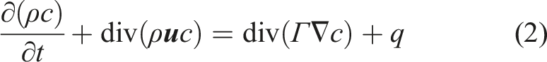
The pollutant concentration at the monitoring point and pollution source was assumed to satisfy the relationship given by equation (1)

$\mathbf{A}\mathbf{q}=\mathbf{C}$

(1)

Where q = [q₁,q₂,q₃,…,q _n ]^T is a n×1 dimension vector that represents the release rate of n pollution sources, C = [C₁,C₂,C₃,…,C _n ]^T is a n×1 dimensional vector that represents the pollutant concentration at n monitoring points. A is a matrix that describes the cause-effect relation between the release rate and the pollutant concentration. Such a cause-effect relation is governed by the scalar transport equation (2).

$\frac{\partial \left(\rho c\right)}{\partial t}+\mathrm{div}\left(\rho \mathit{u}c\right)=\mathrm{div}\left(\Gamma \nabla c\right)+q$

(2)

where ρ is the air density, c is the pollutant concentration, t is time, u is the air velocity, $\Gamma$ is the effective mass diffusivity and q is the source term. The number of monitoring points should the same as that of pollution sources so that matrix A is a square matrix and can be inversely operated. According to equation (1), if the pollutant concentration C and transfer matrix A are known, the release rates for multiple sources can be determined by equation (3)

$\mathbf{q}={\mathbf{A}}^{-1}\mathbf{C}$

(3)

Due to the dissipative characteristics of the forward propagation process and the lagged response of the concentration at the monitoring point, the direct inversion of transfer matrix A is ill-posed. Therefore, Tikhonov regularization method was used to enhance the stability of matrix calculation in equation (3). An objective function (equation (4)) was established to compare the concentration distribution generated by any pollution source with that of monitoring points

$\mathit{Min}\hspace{0.17em}Z\left(\mathit{q}\right)=\Vert \mathit{A}\mathit{q}-{\mathit{C}\Vert }_2^2$

(4)

where ${\Vert .\Vert }_2$ is the Binary norm of matrices. The optimal vector q was obtained by minimizing Z(q). To minimize Z(q), Tikhonov regularization method of equation (5) converts it into an augmented objective function

$\mathit{Min}\hspace{0.17em}Z\left(\mathit{q}\right)=\Vert \mathit{A}\mathit{q}-{\mathit{C}\Vert }_2^2+{\lambda }^2\Vert {\mathit{L}\mathit{q}\Vert }_2^2$

(5)

where λ is a regularization parameter, which directly affects the solved pollutant release rate q.

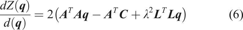
To obtain the minimum of the residual function, the first order derivative of Z(q) with respect to q was calculated, as shown in equation (6)

$\frac{dZ\left(\mathit{q}\right)}{d\left(\mathit{q}\right)}=2\left({\mathit{A}}^T\mathit{A}\mathit{q}-{\mathit{A}}^T\mathit{C}+{\lambda }^2{\mathit{L}}^T\mathit{L}\mathit{q}\right)$

(6)

Further, when d Z(q)/d (q) = 0, the release rate q of gaseous pollutants can be obtained by equation (7)

$\mathit{q}={\left({\mathit{A}}^T\mathit{A}+{\lambda }^2{\mathit{L}}^T\mathit{L}\right)}^{-1}\times {\mathit{A}}^T\mathit{C}$

(7)

where L is regularization matrix and equation (8) is the N-order processing term of q

$\Vert \mathit{L}\mathit{q}{\Vert }^2=\underset{0}{\overset{t}{{\displaystyle \int }}}{\left(\frac{d^N\mathit{q}}{{dt}^N}\right)}^{2}dt$

(8)

where t(s) is the release time of pollution source q. In general, the greater the value of N is, the more favourable it is to eliminate the high-frequency errors of the data. However, at the same time, the smoothness of the data could be damaged. In order to achieve an effective balance between data accuracy and smoothness, N = 2 is usually used. Then L is expressed as equation (9) ³⁷

$L=\left[\begin{array}{cccccccc}1& -2& 1& 0& \cdots & \cdots & \cdots & 0\\ 0& 1& -2& 1& \ddots & \ddots & \ddots & ⋮\\ ⋮& \ddots & \ddots & \ddots & \ddots & \ddots & \ddots & ⋮\\ ⋮& \ddots & \ddots & \ddots & \ddots & \ddots & \ddots & ⋮\\ ⋮& \ddots & \ddots & \ddots & \ddots & \ddots & \ddots & 0\\ 0& \cdots & \cdots & \cdots & 0& 1& -2& 1\end{array}\right]\in R^{(n-2)xn}$

(9)

Choosing a suitable λ becomes the primary concern of the Tikhonov regularisation method. One effective method of finding an optimal λ is to apply the L-curve algorithm. ³⁸ By plotting the log of the norm of regularized term LQ versus the norm of the regularized residual term AQ-C, the curve of L-curve method can be obtained, ³⁹ which is defined by equation (10)

$\left(X\left(\mathit{log}\lambda \right),Y\left(\mathit{log}\lambda \right)\right)=\left(\mathit{log}\Vert \mathit{A}\mathit{Q}-{\mathit{C}\Vert }_2,\mathit{log}\Vert \mathit{L}{\mathit{Q}\Vert }_{\mathbf{2}}\right)$

(10)

The curvature value of each point of L-curve can be obtained by using equation (11), which is the curvature calculation formula of the composite function

$\epsilon \left(\log \mathrm{\lambda }\right)=\frac{X^{\text{'}}{Y}^{\text{'}\text{'}}-X^{\text{'}\text{'}}{Y}^{\text{'}}}{{\left({\left(X^{\text{'}}\right)}^2+{\left(Y^{\text{'}}\right)}^2\right)}^{\frac{3}{2}}}$

(11)

Thus, it is transformed into the problem of selecting the regularization parameter corresponding to the maximum curvature. The $\lambda$ of $\lambda \log \lambda$ matching the maximum curvature of L-curve is the best regularization parameter.

To sum up, with a known transfer matrix A, concentrations C of pollutants at monitoring points, the selected regularization matrix L and the regularization coefficient λ of multiple pollution sources in the artificial environment, the release rate of multiple pollutants can be determined by equation (7). The transfer matrix A is determined by the pollution source contribution rate (CRPS) method.

Contributing factors of pollution source concentration method

After releasing multiple gaseous pollutants, the CRPS index can be introduced to quickly calculate the pollutant concentration at the monitoring point. The principle is that the concentration of pollutants from different sources can be superimposed if the airflow is steady state. ³⁵ As shown in Figure 1, there are various pollutant sources in a room: q₁ is the concentration field generated by the air inlet, q₂ is the concentration field generated by the ceiling, q₃ is the concentration field generated by the floor, and q₄ is the concentration field generated by human beings. The addition of the concentration fields created by q₁, q₂, q₃ and q₄ is equal to the concentration field created by q. CRPS method could directly determine the influence of various pollution sources in the building environment on the distribution of environmental pollutants, simplifies the complex release of multiple pollution sources in the building interior and greatly improves the calculation speed. According to the CRPS method, the transport matrix between release rates of pollution sources and distribution pollutant concentration can be established.

Figure 1.

Schematic diagram of the CRPS method: the release rate of the air inlet, g/s: the release rate of the ceiling, g/s: the release rate of the floor, g/s: the release rate of human beings, g/s.

At the j ^th monitored point, the variation in the concentration caused by the i ^th pollution source is determined by equation (12)

${∆C}_i^j=\frac{q_i}{Q}{CRPS}_i^j$

(12)

where ΔC _i ^j is the contribution of concentration at the j ^th monitored point due to the i^th pollution source, Q is the air flow rate (m³/s). The CRPS factor is dimensionless and constant in the steady-state flow field. CRPS factor is a function of the flow field.

The species transfer equation is a linear system according to the steady flow field in space. The concentration contribution caused by the n pollution sources at a monitored point j is the linear superposition of the concentration contribution caused by each pollution source is defined by equation (13)

${∆C}^j={\displaystyle \sum }_{i=1}^n{∆C}_i^j$

(13)

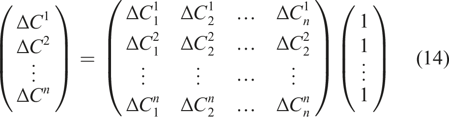
The variation in the pollutant concentration at the monitoring points is described by equation (14)

$\left(\begin{array}{c}{∆C}^1\\ {∆C}^2\\ ⋮\\ {∆C}^n\end{array}\right)=\left(\begin{array}{cccc}{∆C}_1^1& {∆C}_2^1& \dots & {∆C}_n^1\\ {∆C}_1^2& {∆C}_2^2& \dots & {∆C}_2^2\\ ⋮& ⋮& \dots & ⋮\\ {∆C}_1^n& {∆C}_2^n& \dots & {∆C}_n^n\end{array}\right)\left(\begin{array}{c}1\\ 1\\ ⋮\\ 1\end{array}\right)$

(14)

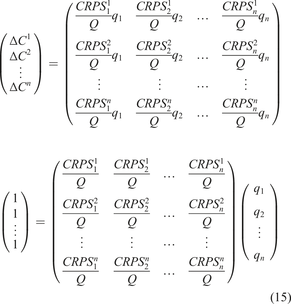
By substituting equation (12) into equation (14), equation (15) is derived

$\left(\begin{array}{c}∆C^1\\ ∆C^2\\ ⋮\\ ∆C^n\end{array}\right)=\left(\begin{array}{cccc}\frac{CRP{S}_1^1}{Q}{q}_1& \frac{CRP{S}_2^1}{Q}{q}_2& \dots & \frac{CRP{S}_n^1}{Q}{q}_n\\ \frac{CRP{S}_1^2}{Q}{q}_1& \frac{CRP{S}_2^2}{Q}{q}_2& \dots & \frac{CRP{S}_n^2}{Q}{q}_n\\ ⋮& ⋮& \dots & ⋮\\ \frac{CRP{S}_1^n}{Q}{q}_1& \frac{CRP{S}_2^n}{Q}{q}_2& \dots & \frac{CRP{S}_n^n}{Q}{q}_n\end{array}\right)\left(\begin{array}{c}1\\ 1\\ ⋮\\ 1\end{array}\right)=\left(\begin{array}{cccc}\frac{CRP{S}_1^1}{Q}& \frac{CRP{S}_2^1}{Q}& \dots & \frac{CRP{S}_n^1}{Q}\\ \frac{CRP{S}_1^2}{Q}& \frac{CRP{S}_2^2}{Q}& \dots & \frac{CRP{S}_n^2}{Q}\\ ⋮& ⋮& \dots & ⋮\\ \frac{CRP{S}_1^n}{Q}& \frac{CRP{S}_2^n}{Q}& \dots & \frac{CRP{S}_n^n}{Q}\end{array}\right)\left(\begin{array}{c}\begin{array}{c}{q}_1\\ q_2\end{array}\\ ⋮\\ q_n\end{array}\right)$

(15)

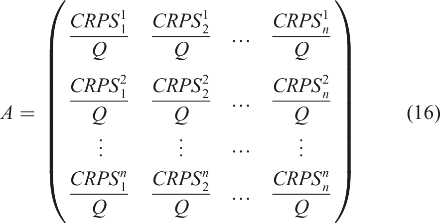
Therefore, the causal transmission matrix A can be expressed by equation (16)

$A=\left(\begin{array}{cccc}\frac{{CRPS}_1^1}{Q}& \frac{{CRPS}_2^1}{Q}& \dots & \frac{{CRPS}_n^1}{Q}\\ \frac{{CRPS}_1^2}{Q}& \frac{{CRPS}_2^2}{Q}& \dots & \frac{{CRPS}_n^2}{Q}\\ ⋮& ⋮& \dots & ⋮\\ \frac{{CRPS}_1^n}{Q}& \frac{{CRPS}_2^n}{Q}& \dots & \frac{{CRPS}_n^n}{Q}\end{array}\right)$

(16)

The process of solution

Figure 2 provides a flowchart for the inverse determination. Firstly, the flow field was obtained by CFD simulation with known environmental parameters. By releasing contaminant at potential source locations, the CRPS distribution of each pollution source was obtained. The above two steps were realized by the ANSYS Fluent. Then, the transmission matrix A between the emission rate of pollution source and the concentration at monitoring points was extracted from the CRPS distribution. Finally, the inverse model, i.e. q = A^-1C, was established to determine the release rate of multiple pollution sources.

Figure 2.

Flow chart for inverse determination of pollutant release rates.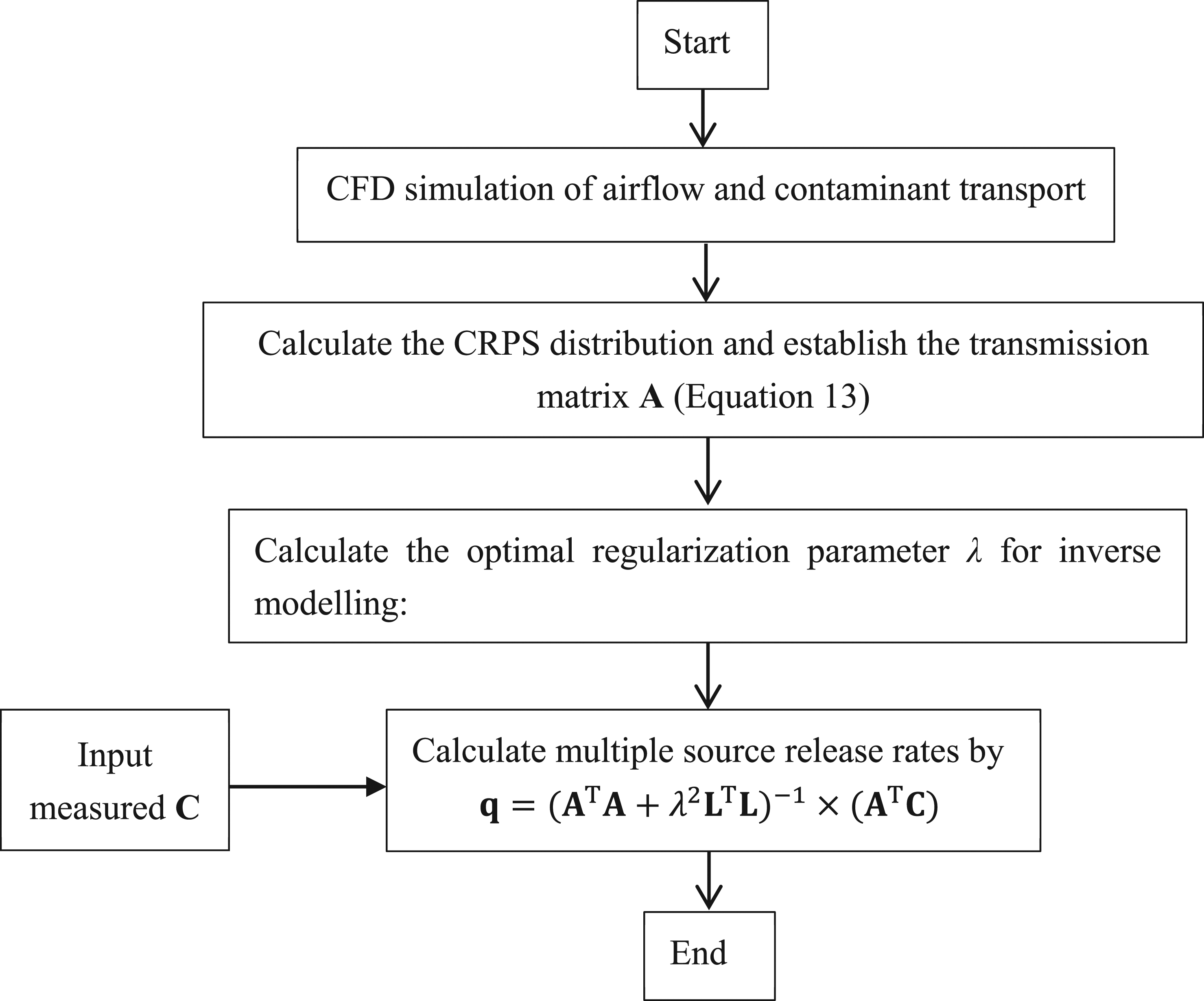

Case setup

This study validated the effectiveness of the inverse determination model by a three-dimensional cavity test bench. ⁴⁰ The validation was to inversely determine the release rates of two gaseous pollution sources in the cavity test bench. The accuracy of the inverse solution was confirmed by comparing results of forward CFD simulation with experimental data. Furthermore, the inverse model was applied to determine release rates of multiple gaseous pollution sources in a three-dimensional cabin.

Three-dimensional cavity test bench

The cavity test bench was 1.8 m long, 1.8 m high and 0.68 m wide as shown in Figure 3. The cavity was insulated by insulation cotton. Air entered the room through a diffuser (0.68 m×0.025 m) in the upper left corner and exited from the exhaust (0.68 m×0.15 m) located at the lower part of the right wall. The model is a simplified model of half an aircraft cabin. In order to simulate an indoor heat source, an empty box (0.4 m×0.68 m×1.1 m) with a 1000 W bulb inside was placed in the lower left corner of the experimental platform.

Figure 3.

Three-dimensional cavity test bench: (a) perspective view and (b) side view.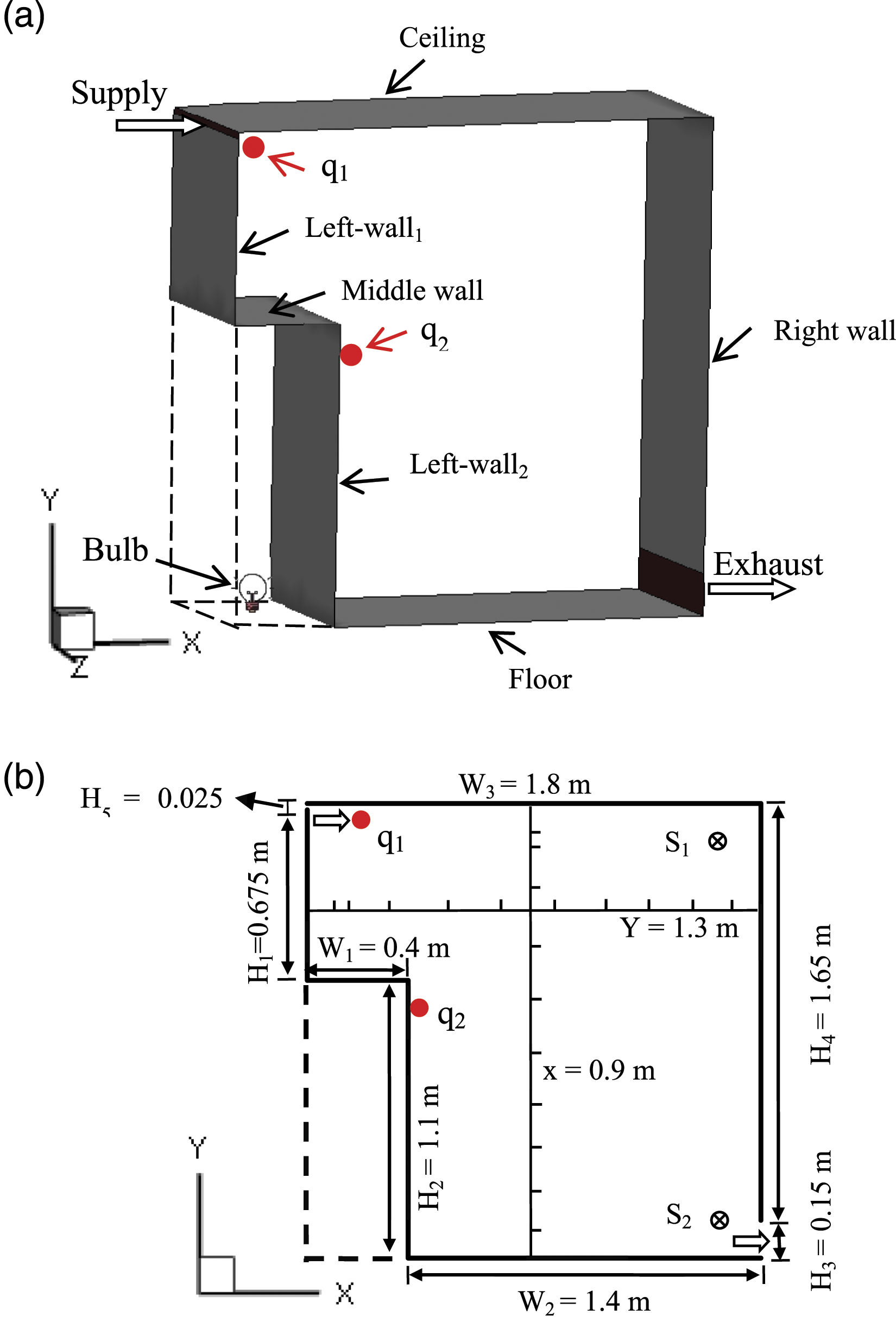

In Figure 3, the red dots represent pollution sources q₁ and q₂. CO₂ was released constantly at these two positions. The releasing port was made of a sponge, so that CO₂ was released with almost zero momentum, reducing the momentum lost when CO₂ was released. In Figure 3(b), the CO₂ concentration was monitored by CIRAS-SC high-precision CO₂/H₂O infrared gas analyzer at S₁ that is at the upper part of the cavity and S₂ that is near the exhaust. The measuring range was 0–9999 µmol/mol, and the nominal measuring accuracy was 0.2 µmol/mol at 300 µmol/mol, 0.5 µmol/mol at 1750 µmol/mol, and 3.0 µmol/mol at 9999 µmol/mol.

The environmental parameters of the cavity were also measured. KIMO VT100s hot wire anemometer was used to measure the air supply velocity. The measuring range of the equipment was 0.15–30.0 m/s, and the measuring accuracy was ±3% reading. The supply air temperature and wall temperature were measured by ZDR-20 temperature and humidity autometer. The temperature measurement range was −40°C–100°C, and the accuracy was ±0.5°C. The environmental parameters of the three-dimensional cavity are shown in Table 1.

Table 1.

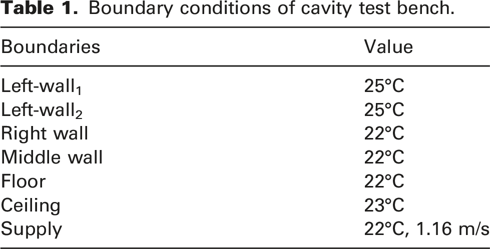
Boundary conditions of cavity test bench.

Boundaries	Value
Left-wall1	25°C
Left-wall2	25°C
Right wall	22°C
Middle wall	22°C
Floor	22°C
Ceiling	23°C
Supply	22°C, 1.16 m/s

In order to validate the simulation, this study measures the air velocity at lines x = 0.9 m and y = 1.3 m. As shown in Figure 3(b), there are 10 measurement points in the vertical direction of x = 0.9 m and the upper horizontal direction of y = 1.3 m in the cavity. The measurements use ultrasonic anemometers DA-650 by Kaijo Sonic, Japan. The velocity measurement resolution was 0.005 m/s with 1% accuracy, and the temperature measurement resolution was 0.025°C with 1% accuracy. At each measuring point, the measurement started after 10 min for stabilization and lasted for 5 min.

Three-Dimensional aircraft cabin model

In order to demonstrate the inverse determination model, this investigation applies the model to an aircraft cabin environment as shown in Figure 4. The release rate of multiple pollution sources in the cabin was determined inversely. The cabin wall was a semi-cylinder with a radius of 2 m and the length of the cabin was 1 m. The air supply diffusers were located at the upper part of the side walls and the airflow rate was 0.03 m³/s. The exhausts were located at the floor level of the side walls. There was one row of seats with six passengers. According to literature, ¹⁸ the environmental parameters of the aircraft cabin during cruise are the surface temperature of human body of 30°C, the wall temperature of 24.5°C, and the seat being adiabatic. The first (q₁) and fourth (q₂) passengers from left to right were assumed to breathe out CO₂ of 0.005 L/s. ⁴¹ CO₂ concentration was monitored at two points S₁ (0.1 m, 0, 0.5 m) and S₂ (2 m,1 m, 0.5 m) as shown in Figure 4.

Figure 4.

Three-dimensional cabin model.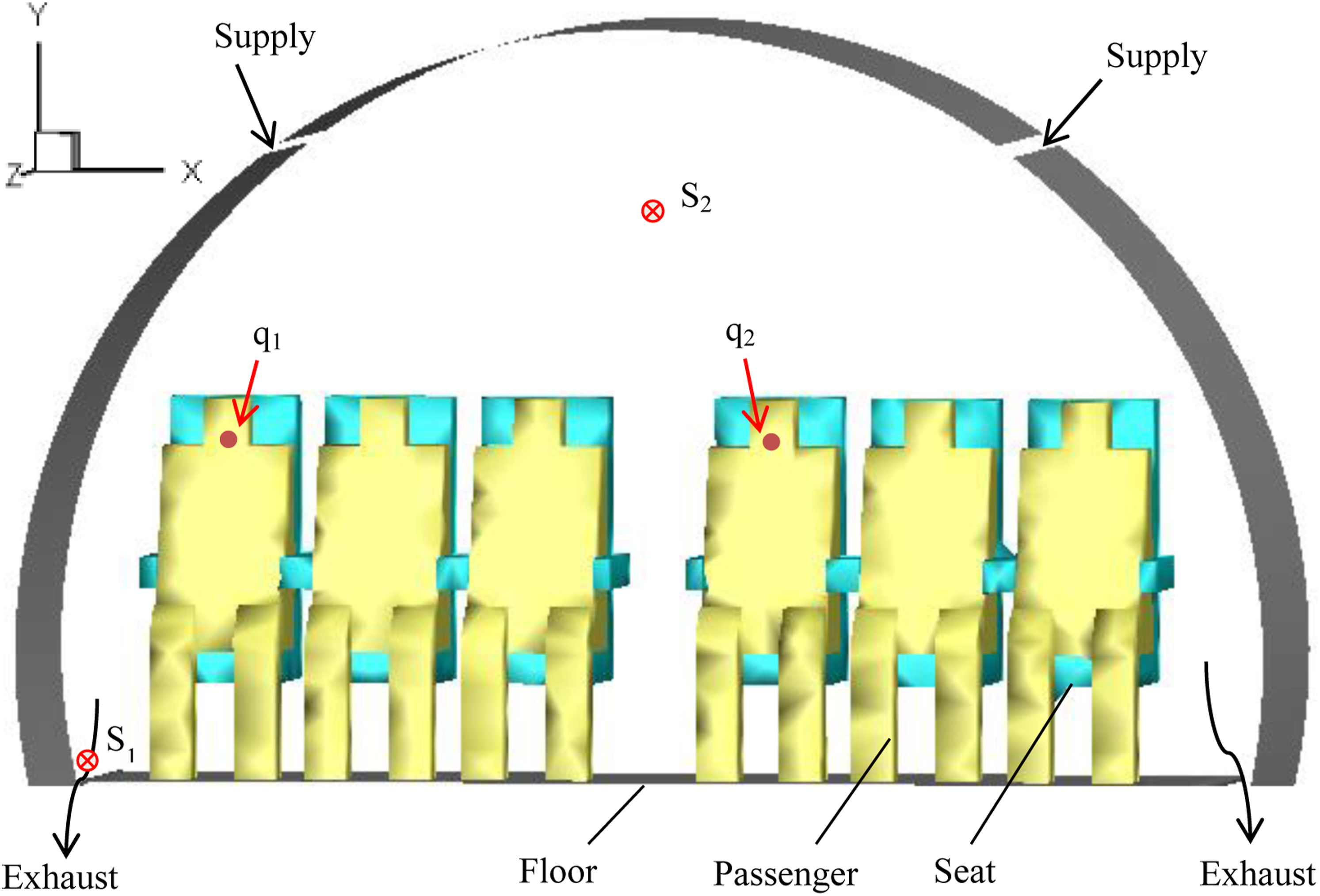

Results and discussion

Three-dimensional cavity test bench

CFD forward simulation

Using the boundary conditions given in Table 1, CFD simulation with the RNG k-ε model in ANSYS Fluent 16.0 was used to solve the airflow in the cavity. Figure 5 shows the air distribution in the cavity. The air was sent through the air supply port on the left side of the cavity top and flows along the wall. Then one large and one small clockwise circulation were generated in the cavity.

Figure 5.

Air distribution in the cavity test bench.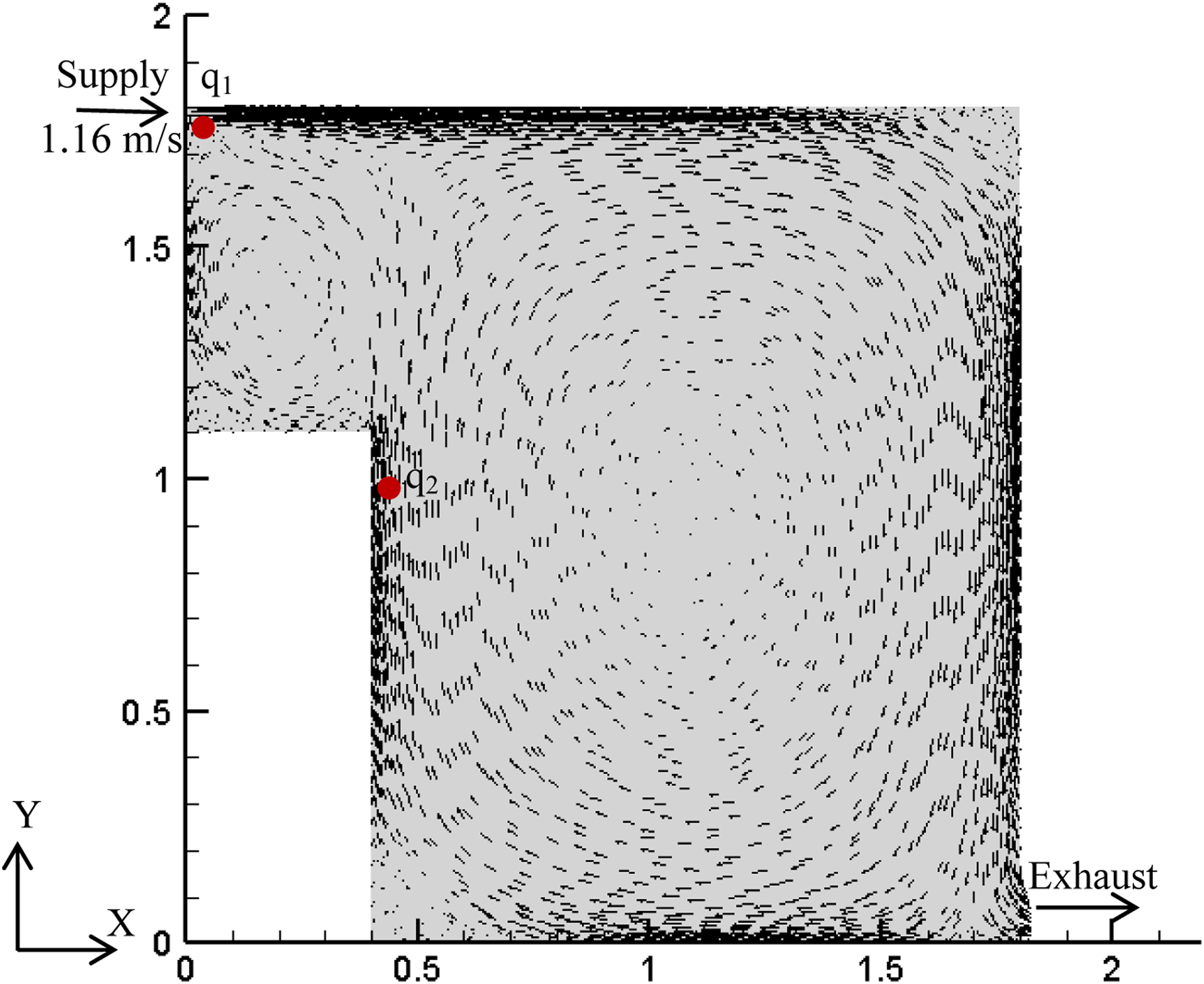

After obtaining the air distribution in the cavity, the air velocity was compared with the velocity measured at the measurement point shown in Figure 3(b). Figure 6 shows the comparison of simulated air velocity and experimental data on horizontal and vertical centre lines in the cavity. There is good agreement between the experimental and simulated air velocity, which, therefore, validated the CFD simulation. Based on the predicted flow field, the concentration response factor under the constant discharge of the pollution source can be solved.

Figure 6.

Comparison between simulated velocity (solid line) and measured velocity (red dots) in the test bench at (a) (b): x = 0.9 m and (c) (d): y = 1.3 m.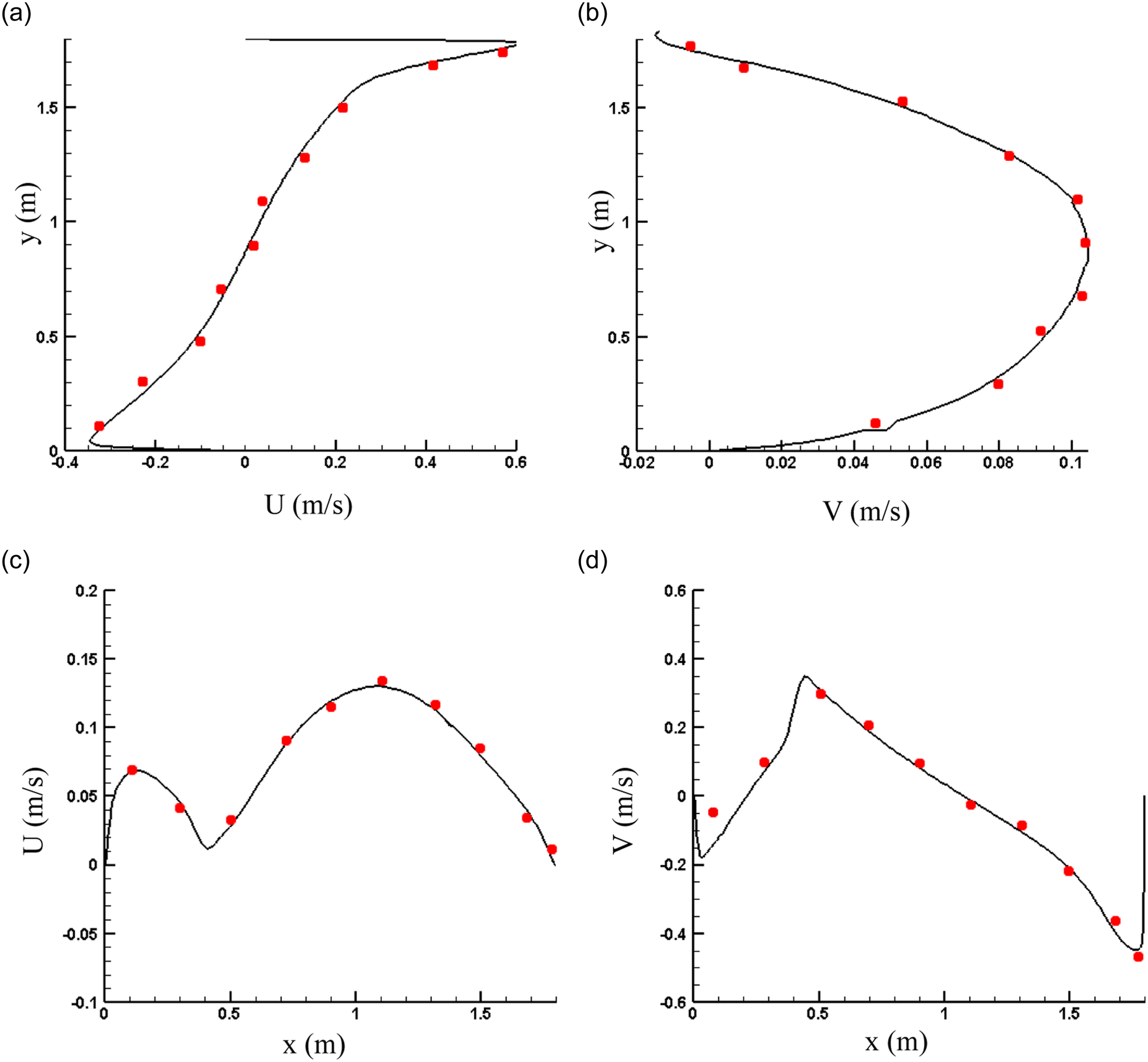

Inverse determination of multiple pollution source release rates

After a steady-state flow field was obtained, CO₂ gas was injected into the cavity with a constant rate of q₁ = 0.1 g/s and q₂ = 0.12 g/s. Figure 7 shows the steady-state concentration distribution of CO₂ for q₁ and q₂, respectively.

Figure 7.

Concentration distribution of CO₂ during steady release in the cavity test bench.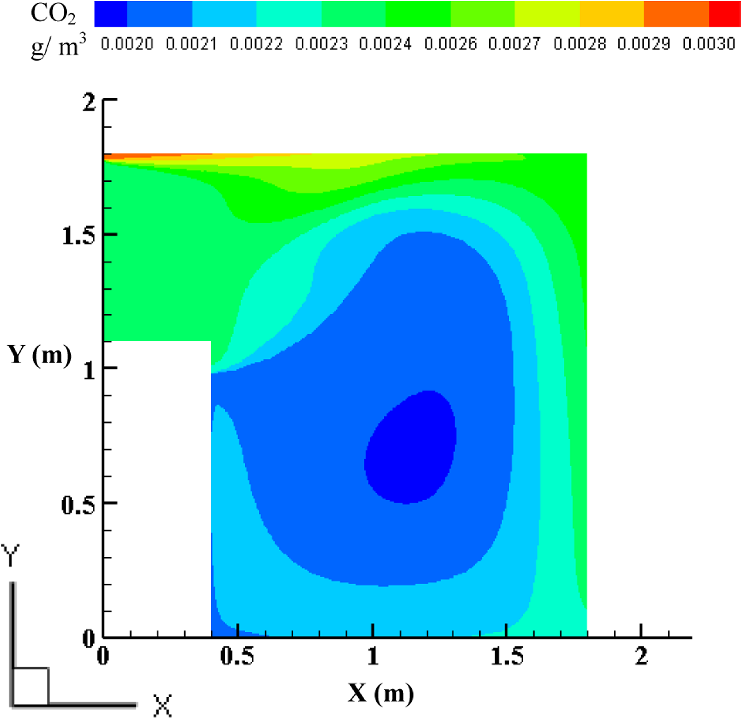

The CO₂ concentration contribution (g/m³) at the monitoring points was determined by equation (17)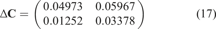

$∆\mathbf{C}=\left(\begin{array}{cc}0.04973& 0.05967\\ 0.01252& 0.03378\end{array}\right)$

(17)

The matrix 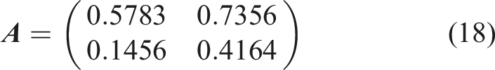A was calculated by equation (18)

$\mathit{A}=\left(\begin{array}{cc}0.5783& 0.7356\\ 0.1456& 0.4164\end{array}\right)$

(18)

To search for an optimal regularized parameter λ, this study adopted a L-curve method. The L-curve method can be regarded as a parameter selection rule as a regularization parameter formula. The relationship between log(λ) and norm (Lq), residual norm (Aq-C) can be found through equation (5). According to literature, L-curve can be smoothed by a cubic spline curve. According to the L-curve theory, the regularization parameter λ was tested in a geometric sequence, to obtain λ = 2.97×10^-2.

From the experimental measurements, the concentration contribution of S₁ and S₂ at steady-state is Δ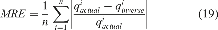C = (0.0599 g/m³ 0.11486 g/m³)^T. After calculation, the release rates of multiple pollution sources in the cavity test bench were q_C = (0.08738 g/s 0.10751 g/s)^T. Then, the MRE (mean relative error) was determined by equation (19)

$MRE=\frac{1}{n}{\displaystyle \sum }_{i=1}^n\left|\frac{q_{actual}^i-q_{inverse}^i}{q_{actual}^i}\right|$

(19)

Where, n is the number of pollution source, $q_{actual}^i$ is the actual release rate of the ith pollution source, $q_{inverse}^i$ is the inverse solution of the ith pollution source. MRE was 11.5% determined by equation (19). The MRE shows that the inverse model has a good accuracy in solving multiple pollution source release rates in the cavity test bench.

Three-dimensional aircraft cabin

Air distribution

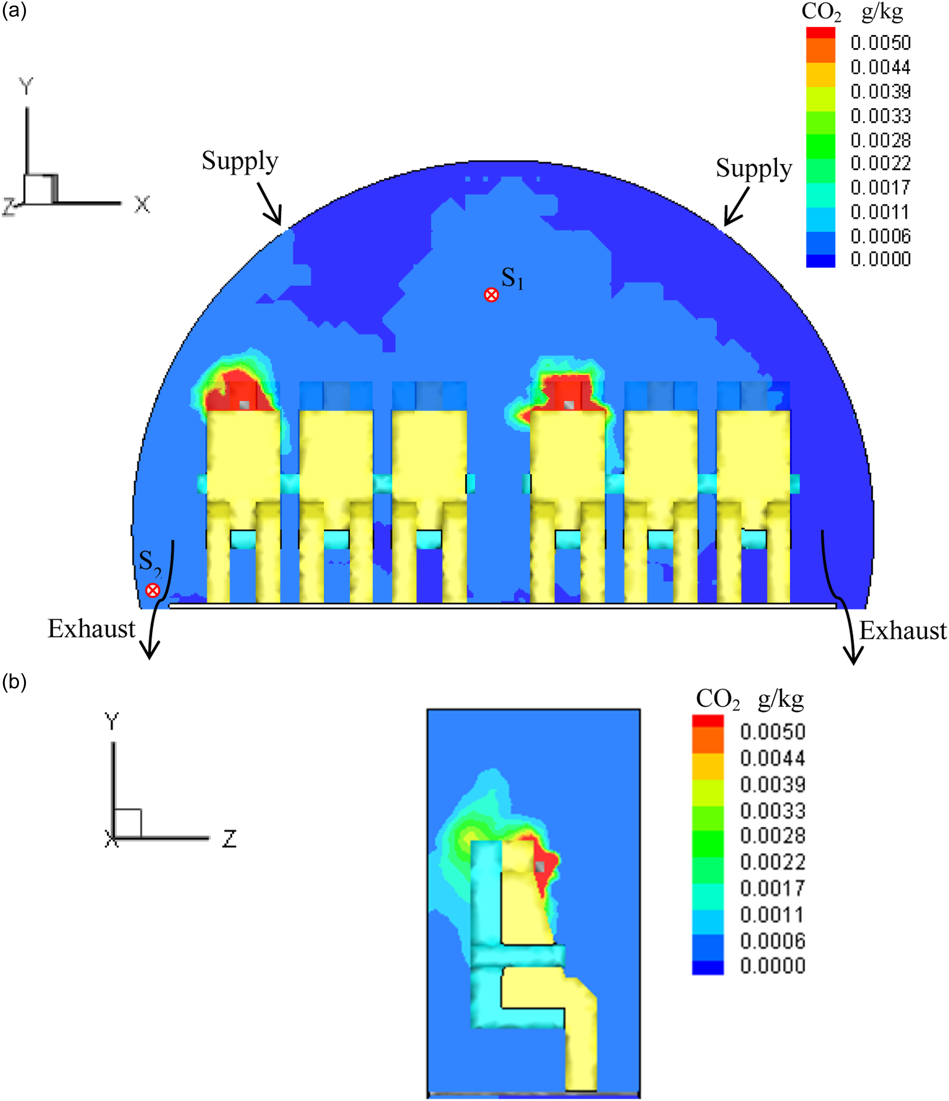
According to the boundary conditions of the cabin, Figure 8 shows the simulated air distribution. The supplied air flowed along the wall surface and produced two approximately symmetrical circulations on both sides of the cabin. Part of the air was discharged to the air outlet along the floor and the rest was re-circulated. CO₂ was released at the first (q₁) and fourth (q₂) passengers with a release rate of 0.005 L/s. Figure 9 shows the CO₂ concentration at planes z = 50 cm and x = 60 cm. Concentrations at monitoring points S₁ and S₂ were ΔC = (0.00449 g/m³, 0.00406 g/m³)^T.

Figure 8.

Air distribution of three-dimensional cabin model.

Figure 9.

Concentration distribution of gaseous pollutants in aircraft cabin at (a) z = 50 cm; (b) x = 60 cm.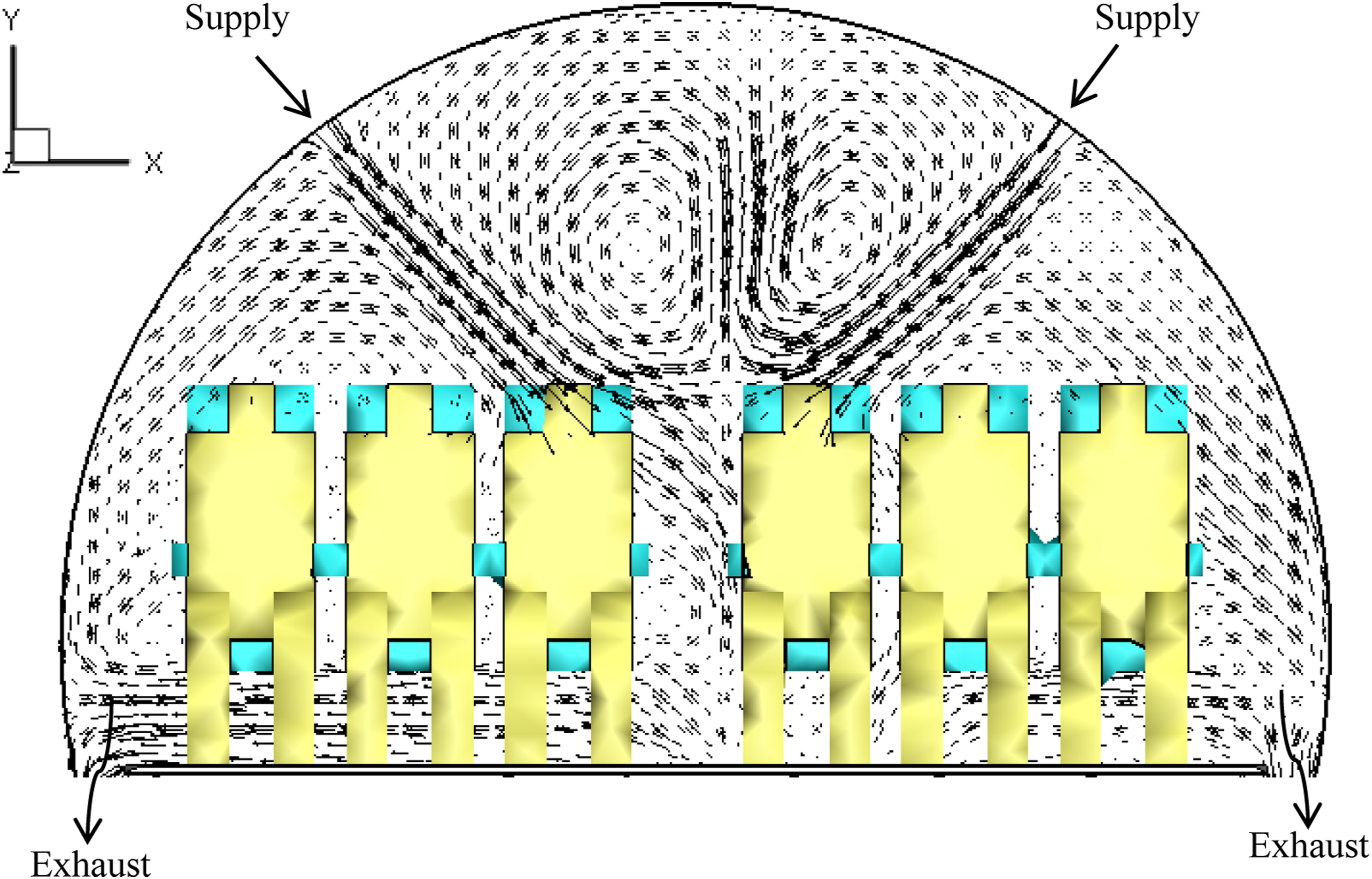

Inverse determination of multiple pollution source release rates in aircraft cabin

According to the pollutant concentration at the monitoring point, the transmission matrix of equation (20) was obtained.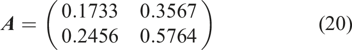

$\mathit{A}=\left(\begin{array}{cc}0.1733& 0.3567\\ 0.2456& 0.5764\end{array}\right)$

(20)

According to the L-curve theory, the regularization parameter λ was tested in a geometric sequence. λ = 0.227 was selected as the optimum regularized parameter. According to equation (5), the release rates of multiple pollution sources in the cabin were obtained qC = (0.00443 L/s 0.00435 L/s)T. Then, the MRE of the pollution source release rate was 12.3% calculated by equation (19).

The calculation result of MRE indicates that applying the inverse model to aircraft cabin can inversely determine the emission rate of multiple pollution sources in the aircraft cabin.

Conclusions

This study has developed an inverse model based on the Tikhonov regularization method to determine the release rate of multiple gaseous pollution sources with the known location of pollution sources. A rapid CRPS method was used to correlate the relationship between the concentration of multiple pollution sources and the monitored pollutant concentrations. The method was validated by experiment in a three-dimensional cavity test bench and was demonstrated by a three-dimensional aircraft cabin test case. The MRE between the actual source strength and the inverse solution were 11.5% and 12.3%, respectively. The results show that this method can accurately determine the emission rate of gas pollution sources in both cases. Although the method was only tested for two sources, it could be applied to scenarios with more sources if there are sufficient number of sensors. In the following work, we can increase the number of pollution sources and monitor points to determine their influence on the calculation results. With the increase in the number of pollution sources and monitor points, the calculation accuracy may be improved, which needs to be confirmed by our next work.