Sage Journals: Discover world-class research

Abstract

A residential building which had been subjected to an energy efficiency measures study had its indoor thermal climate investigated using two software approaches to understand how each approach would predict the outcome, using the predicted percentage of dissatisfied (PPD). The computational fluid dynamics software (ANSYS CFX) and the building performance simulation (BPS) software (IDA ICE) were used to simulate the indoor thermal climate before and after the measures. The measures included additional insulation and changing the ventilation system. The results showed a difference in how the software packages handled the thermal radiation. The difference was also because CFX could calculate the indoor thermal climate of the whole interior. While the PPD values could remain similar between the CFX solutions, the area with dissatisfaction in the apartment was decreased when the building envelope was improved. These changes gave an improvement for the CFX solutions, which was not possible to predict with IDA ICE because only the central node was visible. The user should be aware of the shortcomings of BPS and building energy simulation software when evaluating the indoor thermal climate to predict changes. A coupling between BPS and CFX software should be considered when new measures or significant changes are planned.

Keywords

Energy efficiency measures Indoor thermal climate Sub-Arctic Computational fluid dynamics ANSYS CFX IDA ICE

Introduction

Various studies of renovations and best practice techniques have been performed to investigate possible energy efficiency measures (EEMs) for residential buildings in the colder regions of Sweden, Norway and Finland.^1–5 The most straightforward and simple solution to reduce the heat demand is to improve the building envelope by, for example, adding insulation and new windows. Adjustments of the heating and ventilation systems can also improve the energy efficiency and are often necessary.⁵ These measures, along with others, have been explored from both an energy point of view, life cycle cost and energy and their impacts on the environment.^6–11 However, adjusting the building envelope, heating and ventilation systems will alter the indoor thermal climate. Studies have also detected changes in the thermal climate after renovation⁵,¹² which could have a negative impact on occupants, for example by causing overheating,⁴ which can lead to a rebound effect.¹³,¹⁴ In a region where the heat has to be supplied for most of the year, even a smaller energy loss due to a rebound effect can become significant. EEMs are mainly focused on energy usage and potential economic savings on a life cycle basis, using building energy simulation (BES) or building performance simulation (BPS) tools, and do not necessarily consider the occupants’ perspective. Therefore, it is essential to investigate how possible EEMs will affect the thermal climate inside the building concerned to ensure that the EEMs comply with regulations and at the same time satisfy the requirement for thermal comfort. While BPS software can give an overview of the thermal climate, to ascertain how well this software predicts changes compared to computational fluid dynamics (CFD) software is of interest to academic research and building designers.

When it comes to predicting energy usage, BPS software such as IDA Indoor Climate and Energy (IDA ICE) is popular.⁵,¹²,^15–17 IDA ICE can predict the thermal climate with a reasonable precision.¹²,¹⁸ However, this software, similar to other BPS and BES tools, gives only a rough overview, and may not always predict the correct indoor thermal climate. For each control volume, the equations are solved at the boundaries and in a central node. At the highest resolution, a control volume is usually a room, but could also be an entire floor in a high-rise building. This means that the remaining volume of a room is not accounted for and, therefore, a false impression of the indoor thermal climate can be given. Tian et al.¹⁵ performed a thorough literature review on the subject of BES and CFD and a potential coupling between the two, and pointed out the importance of such a coupling. The advantage of CFD software is that it can investigate the thermal climate on a detailed level. A coupling with BPS can make it possible to investigate a particular scenario or just a specific room.¹⁹ However, CFD software entails a longer setup and computational time, and a general knowledge of CFD is necessary to know how to approach each software package. In addition, the coupling between BES and CFD can be achieved in various ways.¹⁵ Therefore, it is interesting to investigate the differences between the predictions of the thermal climate achieved using BES or BPS and CFD to understand whether CFD is necessary or if BPS is sufficient.

To investigate the indoor thermal climate, the predicted mean vote (PMV) and the predicted percentage of dissatisfied (PPD) models based on ASHRAE Standard 55–2017²⁰ are useful to acquire a good idea of the thermal climate and whether the occupant is dissatisfied due to cold or warm sensations. With CFD, an apartment or even an entire building can be built in 3D. The 3D model is then made into a mesh with smaller control volumes or elements, making a more detailed investigation possible. Using CFD software such as the ANSYS CFX to investigate the indoor thermal climate in full 3D environments with PPD has been shown to be possible.²¹,²² Using a finite volume method such as in ANSYS CFX, each volume is evaluated separately, representing the local thermal climate. By evaluating all of the finite volumes in a room, asymmetries, such as thermal radiation, can be seen and estimates for whole-body thermal sensations would be possible. The study showed that one can conduct a fair assessment for several different scenarios with the same model using CFD and PPD,²³ for example, the scenarios before and after the renovation of a building. The CFD assessment considers three aspects, namely the correct space of the rooms, the severity of discomfort and the time spent in the rooms. The correct space means the occupied zone where people dwell. CFD software enables this approach and can produce results with a higher accuracy than BPS software. The severity of the dissatisfaction is determined based on the PPD percentage. While BPS software can also calculate the PMV and PPD values, CFD software can find these values spatially resolved in the volume. Finally, the time spent in various rooms is essential, since people generally spend more time in bedrooms than in kitchens, for example.²⁴ Both CFD and BPS software can make use of this variable, but CFD can also combine this with results for the whole space.

The CFD solution, however, requires much more computational time to acquire correct results than is required using BPS software. While a finer mesh can give more detailed results, it leads to a longer computational time – perhaps longer than the problem actually warrants. To know that the mesh is designed correctly, it is necessary to perform a refinement study and validate results with measurement data. The user must also know how to set up the solver and how different algorithms can affect the results.

The airflow inside the model can give flows in the laminar, transitional or turbulent region depending on the geometry. While some CFD software may be able to handle the various convection coefficients, some may need user-defined functions (UDFs) to be able to calculate the heat transfer correctly.²⁵ The transition into the turbulent regions requires the use of turbulence models. Rosa et al.²⁶ pointed out that the k-ε turbulence model has been widely used and has been proven to serve well for these types of problems.^27–29 There are also other turbulence models which have been used, such as the SST k-ω turbulence model, when investigating the thermal climate inside a building.³⁰ Setting up the solver for CFD software can end up in a thorough literature review, which may not be the case for BPS software such as IDA ICE. The IDA ICE software has an advanced level and the possibility of the user programming parts of the solver, but the basic level can be sufficient for most cases.

The aim of the present study has been to establish similarities and differences between the BPS software IDA ICE and the CFD software ANSYS CFX when it comes to predicting the indoor thermal climate for residential buildings in sub-Arctic regions. Using CFX for all investigations would be time-consuming, but IDA ICE could, on the other hand, miss important aspects of the indoor thermal climate when EEMs are being investigated. The present study was performed on a building that had been investigated in a previous EEM optimisation study by Shadram et al.,¹ where several scenarios had been investigated using an optimisation algorithm with BPS software. One standard apartment was investigated in this study, and the results obtained using the two software packages were compared.

Methods

The building

The building investigated in the present study is located in the city of Piteå in a sub-Arctic region of Sweden. This building is one of several identical or similar buildings in the area, which were built in the second half of the 1980s and are typical three-storey residential buildings from that time. Due to their age and current heat demand, these buildings are the object of renovation and ongoing EEM investigations.¹ Based on the characteristics of the building, the results and outcomes from the study are expected to be generalised for other similar buildings in the region.

The building has a concrete framework, with timber frames used for the infill, and is insulated with 120–190 mm-thick mineral wool, depending on the section in question, with a 120 mm-thick brick cladding on the outside. The roofs are insulated with 290 mm-thick mineral wool, while the concrete slabs towards the ground are insulated with 60–70 mm-thick styrofoam. The windows are two-layer windows and are currently the section of the building envelope with the highest U-value.

The building is heated with hydronic radiators. The ventilation system is an exhaust air ventilation system where the exhaust air is removed in bathrooms and kitchens. The air is supplied in ducts behind the radiators in bedrooms and living rooms, as illustrated in Figure 1. The radiators heat the incoming cold air to 10°C–15°C. Due to convection forces, some of the air is transported up through the radiator and between the radiator plates. Between these plates, the air is heated further to 20°C–25°C before it is distributed in the room.

Figure 1.

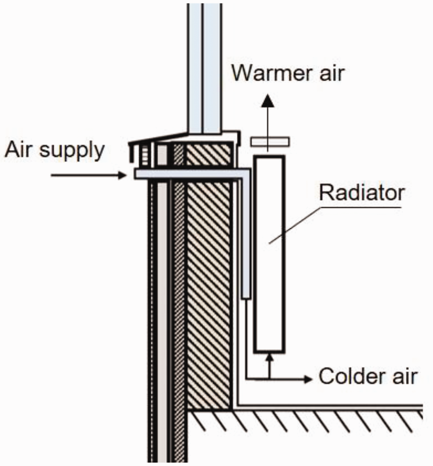
The air supply units in the building.

Indoor thermal climate and data

The heat demand and the possible EEMs were not investigated in the present study since the studied building had already been subjected to EEMs and a life cycle energy study.¹ Instead, the focus for the present study was an investigation of the indoor thermal climate using ANSYS CFX and IDA ICE based on suggested EEMs. Therefore, only one apartment was used instead of the whole building to reduce the computational time for the numerical simulations and to make it possible to validate the models in detail. The data on the building’s properties, such as various dimensions, were gathered from blueprints. The apartment investigated in the present study is typical of the apartments in the building, and its layout is presented in Figure 2.

Figure 2.

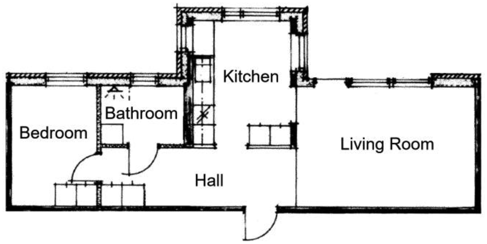
The layout of the apartment in the study.

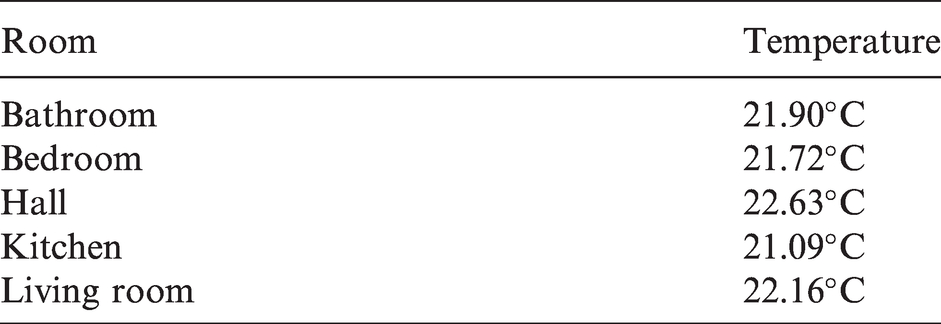
The collected data relating to the thermal climate were the indoor air temperatures, relative humidity, air velocities and surface temperatures. The indoor air temperatures were monitored for one year using temperature gauges mounted on walls. Additional detailed indoor air temperatures, air velocities and surface temperatures were collected for one day in February 2018 for validation of the CFD model. The final temperatures used for the validation of the models for each software package are presented in Table 1. Air-related data were collected in vertical lines in the middle of each room at heights of 0.1, 0.5, 1.0, 1.5 and 2.0 m using a Testo 425 thermal anemometer with an accuracy of ±0.5°C.

Table 1.

Temperatures used for each room.

Room	Temperature
Bathroom	21.90°C
Bedroom	21.72°C
Hall	22.63°C
Kitchen	21.09°C
Living room	22.16°C

The PMV and PPD values according to ASHRAE Standard 55–2017²⁰ were determined and used to evaluate the indoor thermal climate. In all cases, the metabolic rate and clothing were both set to a specific value of 1.0. The value of 1.0 for the clothing represents typical winter indoor clothing, while 1.0 for the metabolic rate represents an occupant being seated and quiet. The relative humidity was set to 8%, which corresponded to the indoor air relative humidity value during the detailed measurement period. The other parameters were derived from the obtained validated solutions.

Since the CFX model was using a finite volume method, the evaluation of the PPD value was possible in every single element, both at a single point in the middle of each room, as in IDA ICE, and in the entire indoor volume. While evaluation of the PPD value at a single point was of interest for the comparison of the two software packages, further evaluation of the CFX model was carried out. Calculating the average values for an entire room can give the wrong impression. Therefore, to assess the occupant’s dissatisfaction more fairly, the assessment followed a previous evaluation of the indoor thermal climate in a study using CFD performed by Lundqvist et al.²³ First, the PPD percentage from 5% to 100% was calculated for each element. A threshold was set to 10%, and people were assumed to be satisfied if the PPD value was lower than 10% in an element, meaning that the element could be excluded from further investigation. Only the volumes within the occupied zone were included for this assessment, where the occupied zone is the zone vertically between 0.1 and 2.0 m, and horizontally 0.6 m from the external surfaces and 0.1 m from the internal surfaces. Using these two conditions, the size of the interior volume where the occupants dwell and experience dissatisfaction was predicted. The derived volume for each room with PPD values above 10% had its average PPD value calculated to evaluate the severity of dissatisfaction in that room. This gave an average PPD value only where dissatisfaction persisted.

Scenarios

The initial models for each software package were created based on the original blueprints for the building envelope, ventilation system and heating system to investigate and predict the thermal climate in a standard apartment. These models are referred to as scenario 1. Another three scenarios were created, numbered 2–4, where additional features were implemented. These features were based on the results of the previously performed study by Shadram et al.¹ By utilising these four separate scenarios, how the two software packages handle changes and predict the indoor thermal climate was investigated. The parameters and their corresponding values used in the four scenarios are described below and summarised in Table 2 for an overview.

Table 2.

Parameters used and their values.

Parameter	Value	Unit
External wall U-value, original	0.16	W/(m² K)
External wall U-value, improved	0.09	W/(m² K)
Window U-value, original	2.00	W/(m² K)
Window U-value, improved	0.80	W/(m² K)
Average supplied air temperature, original	16.75°C
Average supplied air temperature, HRV	19.00°C
Supplied air	1.404 m³/h (0.39 l/s)	per m² floor area
Infiltration	2.88 m³/h (0.80 l/s)	per m² external surface

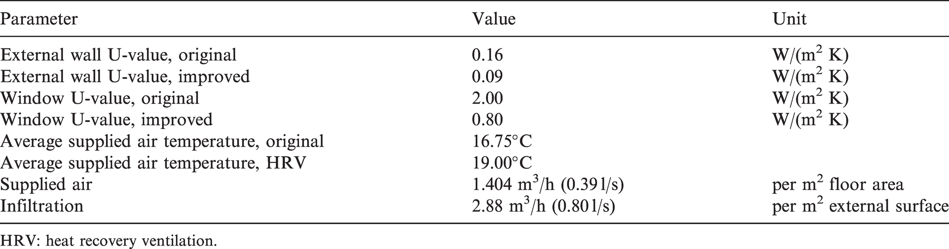
HRV: heat recovery ventilation.

Scenario 1 used the original building envelope with a U-value of 0.16 W/(m² K) for the external walls and 2.0 W/(m² K) for the windows. The exhaust air units in the bathroom and kitchen removed 54 m³/h (15 l/s) each. Regarding the supplied air, 57.6 m³/h (16 l/s) were supplied to the living room and 50.4 m³/h (14 l/s) to the bedroom, which corresponded to 1.44 m³/h (0.4 l/s) per m², floor area. The average temperature of the supplied air after being heated by the radiators was 16.75°C.

In Scenario 2, a 180 mm-thick insulation was added to the external walls and the windows were changed to windows with a U-value of 0.8 W/(m² K). These external changes had been suggested in the previous study by Shadram et al.¹ No additional features were added or changed.

In Scenario 3, the same building envelope as that in scenario 1 was used, but the ventilation system (an exhaust air system) was changed to a system using a heat recovery ventilation (HRV) unit. The supplied air was preheated to 19°C and was led in through internal walls in the bedroom and the living room. This change reduced the stress on the radiators for heating the cold air and could increase the air quality. This measure had also been suggested in the previous study by Shadram et al.¹ The present study does not consider how the HRV and ducts should be installed, or the actual heat exchange.

Scenario 4 was a combination of scenarios 2 and 3. In addition to the 180 mm-thick insulation and better windows being added to the building envelope, the ventilation system was changed to the HRV system.

To compare the outcomes of the different scenarios, an evaluation of the PPD values was made in consideration of the time spent in each room, according to an approach applied in a previous study by Lundqvist et al.²³ A high PPD value in a room where the occupants rarely spend time should not have a significant impact on the overall outcome. The time spent in various rooms was based on a combination of data from the Swedish Standardised and Verified Energy Performance in Buildings (Sveby)³¹ and a study performed by Khajehzadeh et al.²⁴ on the time spent by occupants of dwellings in different rooms. The present study assumed that on average 14 h were spent on a daily basis at home. Out of these 14 h, 8.7 h were spent in the bedroom, 1.6 h in the kitchen, 2.9 h in the living room, 0.7 h in the bathroom and 0.1 h in the hall. The evaluation was carried out for both software packages. For the CFD model, all of the occupied zones were included, as was previously described. The PPD value was multiplied with the percentage of time spent in that room. This combination of time and PPD is referred to as a comparison number henceforth.

Numerical simulation setup

All of the work related to the CFX models was performed with the ANSYS 2019 R3 software. The geometry was based on original blueprints and created as a 3D model with DesignModeler. The apartment was simplified to represent a basic apartment with standard interior fittings such as standard kitchen countertops, home appliances and closets. The windows were extruded from the volume, and the gaps between the rooms were treated as a volume representing the interior walls. The radiators were created as flat surfaces cut out from the interior, but had features added to them on the top and at the bottom to act as inlets. For scenarios 3 and 4, rectangular units were created on inner walls in the living room and bedroom to represent the supply units connected to the HRV. The exhaust units were created as circular openings, one in the bathroom ceiling and one above the stove in the kitchen.

CFX uses a finite volume method, and in the present study, linear elements were used. The mesh was created with the Meshing tool using a maximum cell face length of 0.1 m for the grid size, and all the surfaces of the mesh had inflation layers with a growth rate of 1.5. These settings had previously been proven to be useful for this type of simulation by Risberg et al.²⁷ However, a Richardson extrapolation was performed with four different meshes to make sure that the grid was adequate. The same refinement ratio of 1.4 and the same parameters of temperature and air velocities were used as in the study by Risberg et al.²⁷ The air velocity was sensitive for the solution, while the temperature was one of the most significant parameters for the evaluation of the indoor thermal climate. The cell face length of 0.1 m gave an error of ±0.2°C for the temperature and ±0.02 m/s for the velocity. This error was within an acceptable range, and the cell face length was given a value of 0.1 m. The area for the supply units, exhaust units and radiator surfaces required refinement. All the surfaces acting as inlets for the supply of air had their element size set to 0.01 m. The radiator surfaces had their elemental size set to 0.025 m to calculate the convection correctly.

Only steady-state solutions were used. The setup was defined and the calculation and analysis of the problems were carried out using ANSYS CFX. The simulation consisted of two domains – a fluid domain for the air and a solid domain for the interior walls. The material properties (e.g. conductivity) of the interior walls were set to correspond to the walls in the original apartment. The air velocities were in general 0.1 m/s or lower, resulting in a laminar flow. However, near surfaces, around edges and at the supply and exhaust units, the Reynolds number was high enough to transit into the turbulent region. Following previous CFD studies,²²,²³,²⁵,²⁶ a k–ɛ turbulence model, together with an energy equation, was used.

To be able to investigate the thermal climate in the domain, thermal radiation was included by using a discrete transfer model. All of the participating media within the fluid domain were included, and the solver calculated the total radiative heat transfer. The walls and radiators had their emissivity set to 0.9, and that of the windows was set to a value of 0.83. The radiators’ setup was based on a previous study by Risberg et al.,²⁵ and they were set to transfer the corresponding heat generated by each of them as a heat flux on the front surface, mixing both radiation and convection.

Additional UDFs for the convection heat transfer along surfaces were added to all the surfaces within the domain. The convection coefficients for the external walls, windows and ceiling were based on correlations established by Khalifa and Marshall³² utilising the temperature difference between the domain node and the next node inside the domain. The UDF for the radiators also used the temperature difference, which was a correlation obtained by Alamdari and Hammond.³³ The UDF for the floors used a correlation obtained by Fisher.³⁴ The convection coefficients are summarised in Table 3.

Table 3.

The convection coefficients used for the UDFs.

Surface	Convection coefficient
Floor	$h_{c} = 0.704 + 0.168 {(ACH)}^{0.8}$
Wall	$h_{c} = 2.30 Δ T^{0.24}$
Window	$h_{c} = 8.07 Δ T^{0.11}$
Ceiling	$h_{c} = 3.10 Δ T^{0.17}$
Radiator	$h_{c} = {({(1.5 {(\frac{Δ T}{d})}^{\frac{1}{4}})}^{6} + {(1.23 {(Δ T)}^{\frac{1}{3}})}^{6})}^{1 / 6}$

$Δ T$ is the temperature difference between the surface and the fluid; $d$ is the hydraulic diameter.

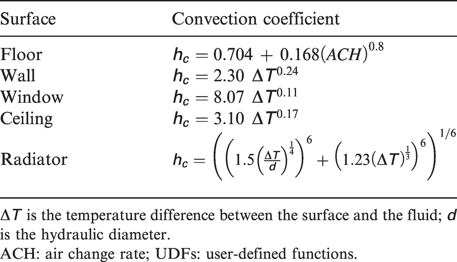
ACH: air change rate; UDFs: user-defined functions.

The boundary conditions for the exterior surfaces were calculated from the U-values for their corresponding heat flux at the time of the specified measurement period. The average temperature in each room and an outdoor temperature of –12.4°C were used. The heat fluxes generated by indirect sunlight, background radiation and radiation from surrounding buildings were calculated and added to the heat fluxes for the respective exterior surfaces. The heat losses due to infiltration were assumed to be uniformly distributed on the exterior surfaces and were included in the boundary condition heat fluxes. Since the apartment was located in the middle of the building, the domain surfaces towards the neighbouring apartments were considered adiabatic. No humans were present in the model, and the heat generated by humans was not included.

The exhaust units removed 54 m³/h (15 l/s) of air, each from the bathroom and the kitchen. The inlet in the bedroom supplied 50.4 m³/h (14 l/s) of air and that in the living room 57.6 m³/h (16 l/s) of air. In scenarios 1 and 3, the settings for the supplied air were approximated as follows: half of the air was supplied above the radiators at 22.5°C, and the other half below the radiator at 11°C. In scenarios 2 and 4, when the HRV was implemented, the temperature of the air supplied from the wall-mounted supply units was 19°C. The setup of the inlets such as boundary and related UDFs were based on a previous work for a building located in the same region.²²

The initial conditions were set to a temperature of 22.0°C, while the pressure and momentum were set to 0 Pa and 0 m/s, respectively. The advection scheme was set to use a second-order upwind term, while the turbulence model used only a first-order term. The use of a first-order term for the latter was due to the way in which CFX handles the turbulence model. The RMS residuals for all of the residuals were set to 10⁻⁴. The relaxation factor was set to 0.5 to avoid oscillations. The initial model, scenario 1, was validated with detailed measurements of air velocities and air temperatures in vertical lines at the centre of each room at heights of 0.1, 0.5, 1.0, 1.5 and 2.0 m.

To calculate the PMV and PPD, expressions were written in CFX-Post. Variables were created to plot the PPD inside the occupied zone for each finite volume with PPD values above 10%. These volumes were filled to identify where problems persisted. Expressions and variables for calculating and plotting the draught rating (DR) are shown in equation (1)

D R = (34 - T_{a}) {(V_{a} - 0.05)}^{0.62} (37 \cdot V_{a} \cdot I_{a} + 3.14)

(1)

In equation (1), $T_{a}$ is the air temperature, $V_{a}$ is the mean air velocity and $I_{a}$ is the turbulence intensity.

IDA ICE model setup

The apartment was created using the IDA ICE 4.8 software. Since the focus of the present study was the indoor thermal climate, the only energy used for the modelling was the heat supplied from the radiators. The geometry and materials for construction elements were based on the original blueprints. The geometry also included the orientation of the apartment.

Scenario 1 was used for validation of the IDA ICE model and, hence, was set up accordingly. The heating setpoint selected for each room was the corresponding measured temperature, with a tolerance of 0.01°C. An air handling unit (AHU) for the supplied air was used for the living room and bedroom, supplying 57.6 m³/h (16 l/s) and 50.4 m³/h (14 l/s) to these rooms, respectively. The average temperature of the supplied air was 16.75°C, and the AHU was set accordingly. An AHU for the return air was used for the kitchen and bathroom, removing 54 m³/h (15 l/s) in each room. Occupants were included for each room to be able to calculate the PMV and PPD values, but their internal gains were set to 0% in order not to interfere with the validation. A heating load simulation with synthetic weather set to the conditions for the specific measurement period was used for the validation. An outdoor temperature of –12.4°C and a clearness of 20% were used. The goal for the validation was to acquire the correct heat supply for the specific day with a maximum error of 5%.

After the validation, these settings remained the same for scenarios 2–4, except for the additional changes described previously for each scenario and the adjusted air velocities and air temperatures. In scenario 2, the construction elements were changed to correspond to the added insulation and changed windows. In scenario 3, the two AHUs were changed to a standard AHU to simulate the HRV unit, supplying air with a temperature of 19.0°C to the room. In scenario 4, all of the EEMs were included. The air velocities and air temperatures in each room were changed for scenarios 2, 3 and 4 to match the results from the corresponding CFX solution at the central node in each room. This method provided both software packages with the same conditions for the indoor thermal climate to determine how well each package predicted the dissatisfaction.

Results and discussion

With the indoor thermal climate in focus, the PPD values are of interest and, therefore, are discussed foremost in this section. The validation process of scenario 1 was successful for both software packages. The IDA ICE model was validated with the heat supply and had a total error of 1% and a maximum error of 5% in the bathroom – representing 17 W. For the CFX model, the velocities and temperatures were used for the validation. Since the velocities were small, the parameters were validated for absolute values instead of percentages. The results were compared with the measured values from the apartment, which showed an overall error of ±0.02 m/s for the velocity and ±0.20°C for the temperatures.

Comparison of the software packages

Since the air temperature and air velocity input for the IDA ICE models were output from the CFX solutions, the main comparison concerned the ways in which each software package handled the results from an indoor-thermal-climate point of view when the same conditions were used. At the central node, the main difference would, therefore, be due to the operative temperature, which was calculated from the mean radiant temperature (MRT).

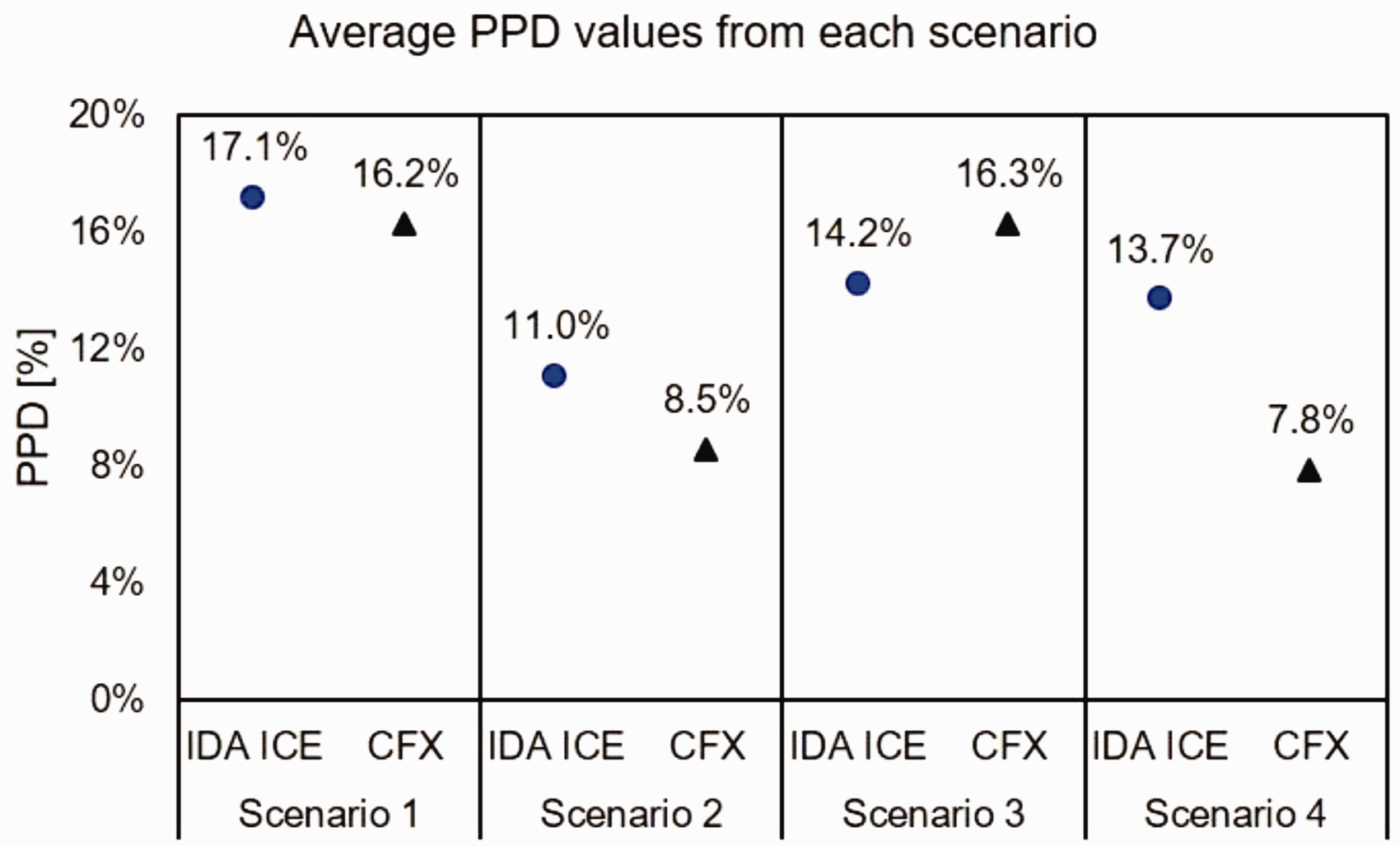
Initially, the PPD value in the central node in each room was extracted. From these values, the average PPD value for each of the four scenarios for both software packages was calculated. These average values – eight values in total – are presented in Figure 3. The differences between IDA ICE and CFX should be noted, with the results from the IDA ICE models being higher than those from the CFX solutions. In scenario 1, the difference was roughly 7%. In the remaining scenarios, there was a persistent 4% difference. This difference between these two software packages was related to the operative temperatures. In scenarios 1 and 3, the CFX solutions had operative temperatures which were higher on average by 1.7°C and 1.3°C, respectively. In these two scenarios, the original building envelope was used and, therefore, the apartment had a higher heat demand. Here the CFX solutions resulted in higher operative temperatures because of warmer surface temperatures mainly attributed to the radiators. In scenarios 2 and 4, when the building envelope was improved, the average difference in the operative temperature dropped to 0.6°C in both scenarios, with CFX still having higher values. These differences in the operative temperatures between the software packages demonstrate how CFX handles surface temperatures and radiation in a different manner from IDA ICE. The resulting temperatures affected the dissatisfaction, and in this case, in favour of the CFX solutions. With the thermal parameters used to calculate the PPD, a difference of 0.5°C in the operative temperature is theoretically enough to make the indoor thermal climate either acceptable or unacceptable when the PPD is used.

Figure 3.

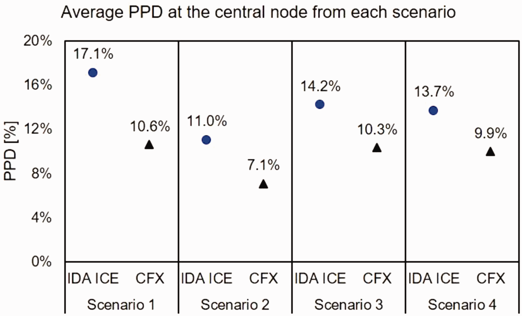
The average PPD values at the central nodes from each scenario, with the dots representing IDA ICE results and the triangles CFX solution results.

The values presented in Figure 3 are average values from the whole apartment in each scenario. Studying the results for each room separately, one can observe that the PPD values range from 5% to about 25% for these two software packages. IDA ICE has higher values in general, ranging from 9% to 22%. On average, the PPD values remained at 14% throughout in all cases. The IDA ICE PPD values from each room are shown in Figure 4. As can be seen, scenario 2 had the lowest PPD values, ranging from 9% to 12%. Scenario 4 had the same building envelope as scenario 2 and gave similar results, except in the bedroom. A 1.3°C temperature difference for both the air temperature and the operative temperature explains the gap between scenarios 2 and 4 in the bedroom. The hall and the kitchen in scenario 1 had higher PPD values of around 20%. These values were due to the lower temperatures, which in scenario 1 were set according to the measured values.

Figure 4.

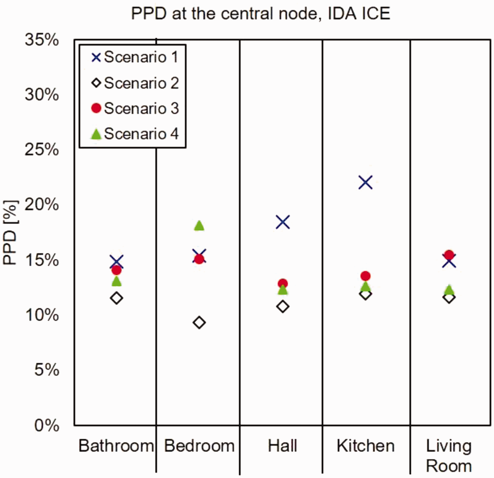
The PPD values from IDA ICE for each room in four scenarios.

The air temperatures set in IDA ICE were first taken from measurements for scenario 1 and then gathered from CFX for the following scenarios. Theoretically, these air temperatures should be adequate, with a mean value of 22°C. The measured temperature in the kitchen was 21°C. However, the operative temperatures were lower than the air temperature in all of scenarios, resulting in negative PMV values in all four scenarios, implying cold sensations. These results suggest that IDA ICE may underestimate the thermal radiation. These PPD values still indicate that IDA ICE predicted an improvement of the indoor thermal climate when the building envelope was improved.

Similar to the presentation in Figure 4, the PPD values from each central node and all rooms given by CFX simulations are presented in Figure 5. As can be seen, the values generally remain lower than those obtained using IDA ICE. The reason for the higher value in the bedroom in scenario 4 was that the point was in the plume from the air supply unit. While the operative temperature was 23°C, the velocity was 0.20 m/s. Neither the placement of the supply unit nor how it should supply air has been considered in this study. However, in scenario 4, CFX could detect the plume and indicate that the supply unit may create dissatisfaction. This is an advantage of the CFD method. The remaining PPD values above 6%, located in the bedroom and living room, had positive PMV values – implying a warm sensation – in contrast to the IDA ICE values. The operative temperatures were higher in the CFX solutions, and these temperatures were calculated from the MRT. Most noticeable was the point in the living room in scenarios 1 and 3 with PPD values of 27% and 31%, respectively. These high PPD values were due to an MRT of around 26°C in both scenarios. The same point in scenarios 2 and 4 gave lower PPD values, 12% and 8%, respectively, and had an MRT of 24°C.

Figure 5.

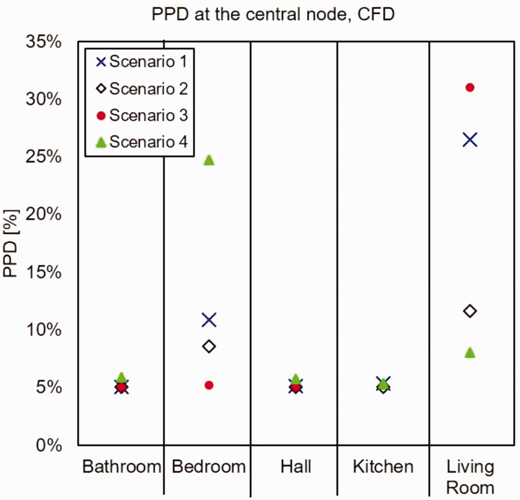
The PPD values at the central node from CFX for each room in the four scenarios.

A comparison of results for the two software packages presented in Figures 4 and 5 indicates a difference in the surface temperatures and how thermal radiation is handled. Although the temperatures used in IDA ICE were gathered from the CFX solutions, there is a clear difference in the PPD values obtained with the two software packages. CFX gave higher MRT values than IDA ICE in all scenarios. The MRT is based on the surface temperatures, which in general were higher in CFX solutions than in IDA ICE models. While the surface temperatures, in general, were close to the air temperature, the temperature of the radiator’s surface, which could reach 50°C, for example, increased the operative temperature to create acceptable PPD values.

The values presented so far show a variation in the outcome between these two software packages. However, outside the central nodes in the CFX solutions, both temperatures and velocities varied. The average PPD values in the occupied zone for the respective scenarios were extracted from the CFX solutions and compared with the IDA ICE values previously presented. The values are plotted in Figure 6, and compared to those in Figure 3, these values show more in common, except for the average values in scenario 4. These values indicate that while the central node in CFX gave reasonable values, the average value inside the whole occupied zone is a better estimate when compared to the IDA ICE results. For scenarios 1, 2 and 3, the difference ranges from 0.9% to 2.5%. In scenario 3, the average PPD value for CFX was higher than that for IDA ICE, which was due to the spike in the living room. With the original building envelope and the HRV system, the occupied zone was subjected not only to a warmer heat supply from the radiator than in scenario 4, but also to a part of the air supply plume. The warmer heat supply created dissatisfaction due to excessively high temperatures, while parts of the room had excessively high velocities. In scenario 4, the average PPD value in the CFX solution was lower than the central node value for IDA ICE. The reason for the decrease in the PPD value, from 9.9% to 7.8%, was due to the previous high PPD value in the bedroom. The central node used previously was located in the air supply plume, which increased the PPD value. By including the occupied zone, the PPD value was decreased.

Figure 6.

Average PPD values from each IDA ICE model (dot), compared with the average PPD values in the occupied zone from each CFX solution (triangle).

Evaluation of the scenarios

In both software packages, only the thermal environment has been investigated in this study. The HRV could potentially increase the air quality and provide other positive outcomes that will not be discussed in the present study.

Combined with the time spent in the rooms, the comparison number was calculated to see overall changes between the scenarios. The results from IDA ICE exhibited similar PPD values throughout all of the scenarios. Due to similar PPD values, and also only the central node was available for results, a comparison between the scenarios where the different amount of time spent in the rooms showed no significant changes. The CFX solutions, on the other hand, showed a more notable change in the PPD values and could also calculate the size of the volume with dissatisfaction inside the occupied zone. The comparison of the indoor thermal climate results from both software packages is shown in Figure 7. While the numbers do not mean anything by themselves, when compared, a lower number indicates that the indoor thermal environment has been improved. The difference in the outcome between IDA ICE (top figure) and CFX (bottom figure) in Figure 7 should be noted.

Figure 7.

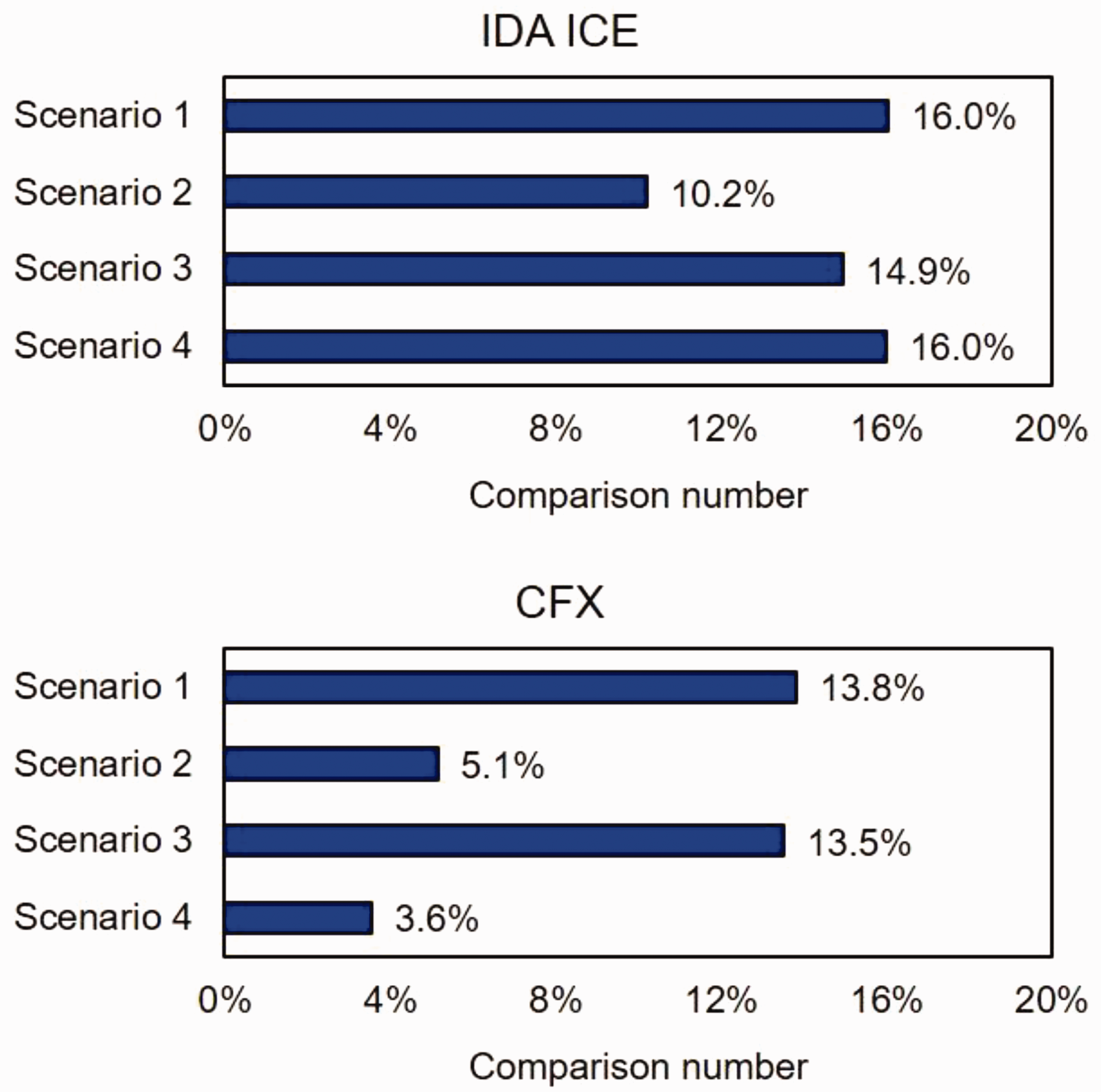
The comparison numbers from IDA ICE (top) and the CFX solutions (bottom).

While IDA ICE indicates that the indoor thermal climate was improved in scenario 2, the remaining three scenarios showed little to no change in the overall indoor thermal climate according to the PPD values. Although scenario 4 had the same building envelope as scenario 2 and only had a different ventilation system, the temperatures were lower in scenario 4 than in scenario 2, as previously mentioned. The lower temperature resulted in a lower operative temperature, which gave higher PPD values. These PPD values could, of course, be improved by increasing the temperatures to a level on par with those in scenario 2. However, for the sake of comparing the two software packages, the same conditions were used. As previously discussed, the difference was mainly related to the MRT.

On average, the most significant improvement in the IDA ICE models was made in the kitchen, followed by the hall. These two rooms are rooms where occupants spend less time than they do in the bedroom – a room that had an increase in the PPD value in scenario 4. These values resulted in no real improvement for the IDA ICE scenarios from scenario 1 to 4.

The CFX solutions, however, showed a significant improvement from scenario 1 to 4, as seen in Figure 7. The significant change in the comparison number in Figure 7 was due to the volume with dissatisfaction. In scenario 1, the volume where the PPD values were larger than 10% represented 54.4% of the occupied zone, whereas, in scenario 4, the corresponding volume had decreased to 14.7% of the occupied zone. In Figure 7, scenario 2 showed an improvement, while scenario 3 was similar to scenario 1. With a thicker building envelope, the heat supply from the radiators was reduced, which resulted in a lower MRT and an improved indoor thermal environment. The previously presented PPD values in the central node in Figure 3 showed a minor improvement from scenario 1 to 4, which was actually not the case. The thicker building envelope had the most significant impact on the indoor thermal environment.

Analysis of the CFX solutions

The present study did not aim to find an optimal solution for the HRV supply units or define which EEM is the best. Therefore, these topics are not discussed in greater detail in this paper. The scenarios and their outcomes are, however, presented and discussed to give an overview of the CFD solutions. In all of the scenarios, full 3D models were used. The rendered volumes of PPD values above 10% in scenarios 1 and 4 are shown in Figures 8 and 9, respectively, to demonstrate the results. As can be seen in both figures, some of the volumes in the interior were filled. The PPD value was calculated in each element, but only those above 10% were filled. The two figures demonstrate the improvements made from scenario 1 to scenario 4.

Figure 8.

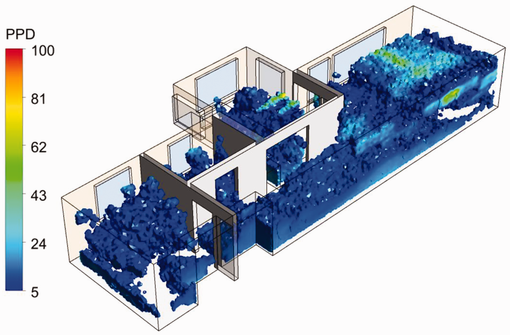
3D view of the CFX solution, scenario 1, with the PPD volumes.

Figure 9.

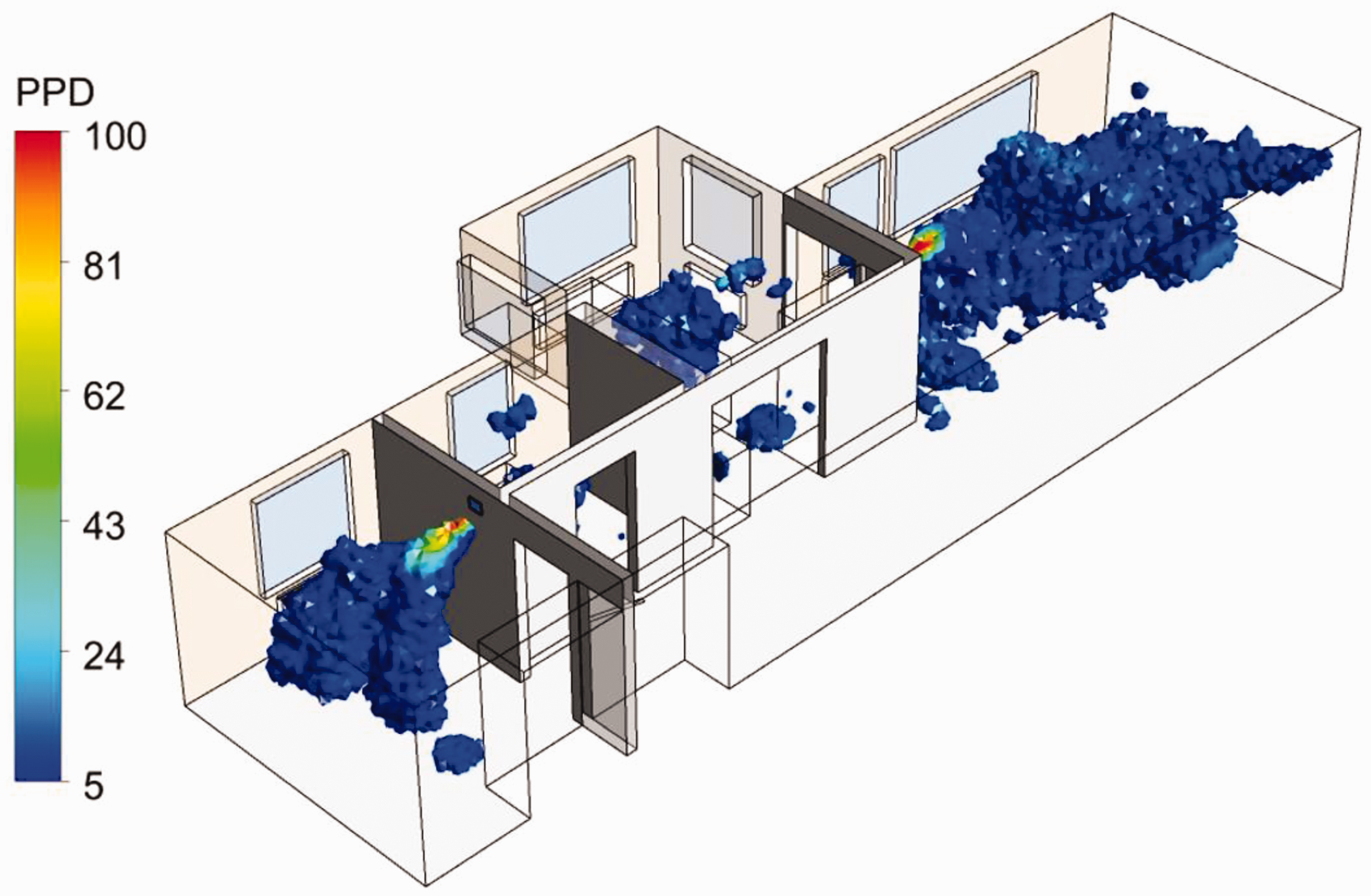
3D view of the CFX solution, scenario 4, with the PPD volumes.

In the four scenarios, the temperatures varied between 17°C and 24°C in the occupied zone. The lower temperatures persisted in scenarios 1 and 2 near the floor in the bedroom and living room, close to the supply unit below the radiator, which was expected. The higher temperatures were present in all of the scenarios at the top of the occupied zone and in the area closest to the radiators, and this was also expected. On average, the air temperature was 22°C inside the occupied zone. The velocities varied between 0.01 and 0.81 m/s in the occupied zone, with an average of 0.03 m/s. The higher velocities were near the HRV supply units due to the plume, as previously described. Only scenarios 3 and 4 had some significant DRs which should raise concern and further investigation. The draught in the living room in these two scenarios was the most significant factor from a dissatisfaction point of view. The DR created by the plume from the supply units located in the living room in scenarios 3 and 4 is shown in Figure 10. As can be seen, the colder air entered the room from the supply unit, and the plume was formed as a downward curve. The plume from the supply unit added to the dissatisfaction in the living room mainly due to higher air velocities.

Figure 10.

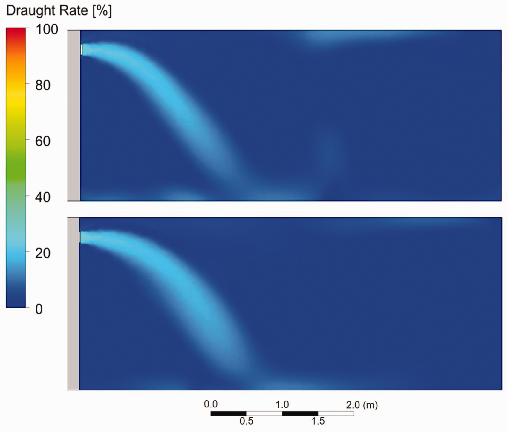
2D plane of the DR in the living room for scenario 3 (top) and scenario 4 (bottom).

The images in Figure 10 show that the CFX solution has a clear advantage over IDA ICE. Based on these images, it would be possible to investigate further the various placements of the supply unit, the shape of the supply unit and different flows to create a better indoor thermal climate. Moreover, the images support to make a better assessment of the severity of the dissatisfaction. While the average PMV and PPD values in the occupied zone, or central nodes in a room, indicate the dissatisfaction, the CFX solutions can be evaluated further, similarly to the evaluation of the scenarios.

To exemplify this, one can compare scenarios 3 and 4. In the occupied zone, scenario 3 had an average PPD value of 16%, while scenario 4 had a corresponding value of 8%, which implies that scenario 4 was better in this case. However, it is also possible to calculate the number of finite volumes inside the occupied zone with PPD values above 10% and where dissatisfaction persisted. Scenario 3 had dissatisfaction in 47% of the occupied zone, while scenario 4 had dissatisfaction only in 15% of the occupied zone. From this perspective, scenario 4 had an improved indoor thermal environment. The location of these volumes also matters. As observed earlier, the living room in scenario 3 had a higher PPD value in the central node, a PPD of 31%. The remaining rooms in scenario 3 had PPD values of around 5%. On the other hand, in scenario 4, the dissatisfaction was mainly in the bedroom, which was indicated in Figure 5 by a PPD value of 25%. Since the occupants tend to spend more time in the bedroom, this could affect the outcome if the occupied zones had a similar dissatisfaction overall.

These aspects, in addition to the possibility of investigating the interior in a greater detail, mean that using a CFD method can provide tangible benefits. Therefore, CFD should be considered in some aspects and be coupled with BPS software, such as IDA ICE in this case. Some software packages for both CFD and BPS/BES can use CAD models as input, making it possible to use the same model. However, CFD requires meshing of the model which requires a grid size study, unless there is an assumption that a predetermined grid size is correct. Even with automated meshing tools and standardised, validated methods, the CFD method is time-consuming and should be saved for specific cases.

Conclusions

The use of BPS tools like IDA ICE coupled with CFD software has already been presented and explored in previous research studies. The present study explored a residential building in a sub-Arctic region to understand how BPS and CFD software evaluate the indoor thermal environment and predict future changes based on suggested EEMs. The combination of BPS software like IDA ICE with CFD software is an essential step in developing research in this field further and understanding the indoor thermal climate better.

The two software packages investigated in the present study did not predict the same indoor thermal climate. While similarities could be seen when the average values for the whole occupied zone obtained with CFX were compared with those obtained with IDA ICE, the overall results showed differences, mainly attributed to the radiant temperatures. CFX was able to include the interior to a much greater detail and evaluate the thermal radiation differently from IDA ICE. Though the calculations of the MRT by the two software packages were performed accurately, the surface temperatures were different and hence different results were obtained. IDA ICE did not detect the temperature variation originating in the warmer surfaces of radiators in the same manner as CFX, for example. The residential buildings in the sub-Arctic region require significant heating compared to many other regions. Some BPS and BES software packages might not handle the increased thermal radiation from the radiators correctly. CFX was also able to detect issues and could pinpoint where they persisted, which the IDA ICE software could not. In a future study, CFD could be used to investigate HRV and to find a better placement and shape of the supply units, and study the effect of various flow fields to improve the indoor thermal climate further.

However, the use CFX or other CFD software as a tool requires not only knowledge of the software, but also a broad knowledge of CFD in general if one is to be successful in meshing, setting up the problem and postprocessing. The purpose of BPS tools like IDA ICE is to investigate the energy and thermal performance of buildings, while CFD software such as CFX is not explicitly designed for that. BPS tools like IDA ICE are more accessible for engineers within their specific fields. The users of such tools should, however, be aware of possible shortcomings of these tools when evaluating the indoor thermal climate for buildings located in the sub-Arctic region. Coupling BPS and CFD and working with a combination of both should be considered when evaluating specific scenarios such as extreme conditions, new technology and significant EEMs, to evaluate the indoor thermal climate better.

Footnotes

Acknowledgements

The authors would like to thank the housing company AB PiteBo for letting us work with their buildings and made this research possible. Also thanks to our academic partners at Luleå University of Technology.

Authors' contribution

PL: Concept, methodology, investigation, writing; MR: Concept, methodology, writing, funding acquisition; LW: Concept, writing, funding acquisition.

Declaration of conflicting interests

The author(s) declared no potential conflicts of interest with respect to the research, authorship, and/or publication of this article.

Funding

The author(s) disclosed receipt of the following financial support for the research, authorship, and/or publication of this article: This work was supported by the EU program Interreg Nord, Region Norrbotten and Luleå University of Technology.

ORCID iDs

Petter Lundqvist

Mikael Risberg

References

Shadram

Bhattacharjee

Lidelöw

Mukkavaara

Olofsson

Exploring the trade-off in life cycle energy of building retrofit through optimization. Appl Energy 2020; 269: 115083.

Mattinen

Tainio

Salo

Jalas

Nissinen

Heiskanen

How building users can contribute to greenhouse-gas emission reductions in Finland: comparative study of standard technical measures, user modifications and behavioural measures. Energy Effic 2016; 9: 301–320.

Allard

Olofsson

Hassan

OAB.

Methods for energy analysis of residential buildings in Nordic countries. Renew Sustain Energy Rev 2013; 22: 306–318.

Ayikoe Tettey

Gustavsson

Energy savings and overheating risk of deep energy renovation of a multi-storey residential building in a cold climate under climate change. Energy 2020; 202: 117578.

Lundqvist

Risberg

Westerlund

The importance of adjusting the heating system after an energy-retrofit of buildings in a sub-Arctic climate. Energy Build 2020; 217: 109969.

Nydahl

Andersson

Åstrand

Olofsson

Environmental performance measures to assess building refurbishment from a life cycle perspective. Energies 12: 299.

Mukkavaara

Sandberg

Pousette

Norén

Sustainability evaluation of timber dwellings in the north of Sweden based on environmental impact and optimization of energy and cost. Procedia Manuf 2020; 44: 76–83.

Ramírez-Villegas

Eriksson

Olofsson

Combined environmental and economic assessment of energy efficiency measures in a multi-dwelling building. Energies 12: 2484.

Ramírez-Villegas

Eriksson

Olofsson

Life cycle assessment of building renovation measures–trade-off between building materials and energy. Energies 2019; 12: 344.

10.

Lidelöw

Örn

Luciani

Rizzo

Energy-efficiency measures for heritage buildings: a literature review. Sustain Cities Soc 2019; 45: 231–242.

11.

Piccardo

Dodoo

Gustavsson

Tettey

UYA.

Retrofitting with different building materials: life-cycle primary energy implications. Energy 2020; 192: 116648.

12.

La Fleur

Moshfegh

Rohdin

Measured and predicted energy use and indoor climate before and after a major renovation of an apartment building in Sweden. Energy Build 2017; 146: 98–110.

13.

Brøgger

Bacher

Madsen

Wittchen

KB.

Estimating the influence of rebound effects on the energy-saving potential in building stocks. Energy Build 2018; 181: 62–74.

14.

Rau

Moran

Manton

Goggins

Changing energy cultures? Household energy use before and after a building energy efficiency retrofit. Sustain Cities Soc 2020; 54: 101983.

15.

Tian

Han

Zuo

Sohn

MD.

Building energy simulation coupled with CFD for indoor environment: a critical review and recent applications. Energy Build 2018; 165: 184–199.

16.

Liu

Rohdin

Moshfegh

Evaluating indoor environment of a retrofitted multi-family building with improved energy performance in Sweden. Energy Build 2015; 102: 32–44.

17.

Milić

Ekelöw

Moshfegh

On the performance of LCC optimization software OPERA-MILP by comparison with building energy simulation software IDA ICE. Build Environ 2018; 128: 305–319.

18.

Andersen

Fabi

Corgnati

SP.

Predicted and actual indoor environmental quality: verification of occupants’ behaviour models in residential buildings. Energy Build 2016; 127: 105–115.

19.

Barbason

Reiter

Coupling building energy simulation and computational fluid dynamics: application to a two-storey house in a temperate climate. Build Environ 2014; 75: 30–39.

20.

ANSI/ASHRAE Standard 55-2017. Thermal environmental conditions for human occupancy. Atlanta: The American Society of Heating, Refrigerating and Air-Conditioning Engineers, 2017.

21.

Yang

Thermal comfort analysis of a high-speed train cabin considering the solar radiation effects. Indoor Built Environ 2020; 29: 1101–1117.

22.

Risberg

Westerlund

Investigation of thermal indoor climate for a passive house in a sub-Arctic region using computational fluid dynamics. Indoor Built Environ 2019; 28: 677–692.

23.

Lundqvist

Risberg

Westerlund

Air heating system design for a sub-Arctic climate using a CFD technique. Build Environ 2019; 160: 106164.

24.

Khajehzadeh

Vale

Isaacs

Time-use in different rooms of selected New Zealand houses and the influence of plan layout. Indoor Built Environ 2018; 27: 19–33.

25.

Risberg

Westerlund

CFD modelling of radiators in buildings with user-defined wall functions. Appl Therm Eng 2016; 94: 266–273.

26.

Rosa

Soares

Costa

Santos

Gervásio

Assessment of an earth-air heat exchanger (EAHE) system for residential buildings in warm-summer Mediterranean climate. Sustain Energy Technol Assessments 2020; 38: 100649.

27.

Risberg

Westerlund

Hellstrom

JGI.

Computational fluid dynamics simulation of indoor climate in low energy buildings computational set up. Therm Sci 2017; 21: 1985–1998.

28.

Nielsen

PV.

Fifty years of CFD for room air distribution. Build Environ 2015; 91: 78–90.

29.

Gupta

Khare

VR.

Natural ventilation design: predicted and measured performance of a hostel building in composite climate of India. Energy Built Environ 2021; 2: 82–93.

30.

Javad

Navid

Thermal comfort investigation of stratified indoor environment in displacement ventilation: climate-adaptive building with smart windows. Sustain Cities Soc 2019; 46: 101354.

31.

Sveby. Brukarindata bostäder. Stockholm, http://www.sveby.org/wp-content/uploads/2012/10/Sveby_Brukarindata_bostader_version_1.0.pdf (2012, accessed 4 July 2019).

32.

Khalifa

AJN

Marshall

RH.

Validation of heat transfer coefficients on interior building surfaces using a real-sized indoor test cell. Int J Heat Mass Transf 1990; 33: 2219–2236.

33.

Alamdari

Hammond

GP.

Improved data correlations for buoyancy-driven convection in rooms. Build Serv Eng Res Technol 1983; 4: 106–112.

34.

Fisher

DE.

An experimental investigation of mixed convection heat transfer in a rectangular enclosure. PhD Thesis, University of Illinois, Illinois, US, 1995.

Indoor thermal climate after energy efficiency measures of a residential building in a sub-Arctic region: Comparing ANSYS CFX and IDA ICE methods

Abstract

Keywords

Introduction

Methods

The building

Indoor thermal climate and data

Scenarios

Numerical simulation setup

IDA ICE model setup

Results and discussion

Comparison of the software packages

Evaluation of the scenarios

Analysis of the CFX solutions

Conclusions

Footnotes

Acknowledgements

Authors' contribution

Declaration of conflicting interests

Funding

ORCID iDs

References