Mixing ventilation driven by two oppositely located supply jets with a time-periodic supply velocity: A numerical analysis using computational fluid dynamics

Abstract

Ventilation is of primary importance for the creation of healthy and comfortable indoor environments and it has a significant impact on the building energy heating and cooling demand. The aim of this study is to assess the application of time-periodic supply velocities to enhance mixing in mixing ventilation cases to reduce heating and cooling energy demands. This paper presents computational fluid dynamics (CFD) simulations of a generic mixing ventilation case, in which the time-averaged velocities and pollutant concentrations from a reference case with constant supply velocities were compared with those obtained from a case with time-periodic supply velocities (sine function). The unsteady Reynolds-averaged Navier-Stokes (URANS) CFD simulations indicate that the use of time-periodic supply velocities can reduce high pollutant concentrations in stagnant regions, reduces the overall time-averaged pollutant concentrations and increases contaminant removal effectiveness with about 20%. The influence of the period of the sine function was assessed and the results showed that for the periods tested, the differences are negligible. Finally, the URANS approach was compared with the large eddy simulations (LES) approach, indicating that URANS leads to very similar results (NMSE < 3.2%) as LES and can thus be regarded as a suitable approach for this study.

Introduction

Ventilation is essential to obtain a healthy indoor environment in buildings, but also in other enclosures such as cars and airplanes. The amount of ventilation (ventilation rate (m³/s)) and the ventilation efficiency (e.g. air exchange effectiveness, contaminant removal effectiveness (CRE)) both have a large influence on the indoor air quality, and together with indoor pollutant sources and sinks determine the overall indoor air quality in an enclosure. A sufficient ventilation rate is required to keep the pollutant concentrations, air temperature and relative humidity in an enclosure at acceptable levels. However, too high supply volume flow rates should be avoided in the case of mechanical ventilation since it uses energy for heating/cooling of the supply air and for fan operation. Also, in naturally ventilated buildings the ventilation rate should be controlled to limit the energy losses. To provide healthy indoor environments and simultaneously reduce energy demand, it is of primary importance to ventilate buildings and other enclosures as efficiently as possible. One possibility for the enhancement of the overall ventilation efficiency, at least in mixing ventilation cases, is the application of time-periodic supply velocities (i.e. supply flow rate) instead of constant supply velocities. The use of time-periodic supply velocities could result in enhanced mixing due to the expected breakup of recirculation cells and movement of stagnant regions throughout the enclosure. An enhanced amount of mixing in an enclosure could lead to a reduction of the required supply volume flow rates and thus of the required energy consumption, without compromising the indoor air quality, and would thus be beneficial with respect to both building energy demand and indoor air quality. Additional advantages can be found in an enhanced appreciation of the thermal conditions inside the enclosure, since time-periodic supply velocities might lead to flow characteristics (e.g. turbulence intensity, power spectra) that resemble the characteristics of natural ventilation flows. Fluctuating or intermittent ventilation flows are considered to be favourable in warm/hot conditions (cooling conditions), due to their inherent transient nature, with temporal variations in velocity and turbulence.^1–4

In the past decade, a few papers on time-periodic forcing for ventilation purposes have been published. Schmidt et al. ⁵ studied the airflow patterns in a generic rectangular enclosure resulting from the instationary operation of the available mixing ventilation system. Their results indicated a more uniform time-averaged velocity distribution when time-periodic supply velocities were used than in the case of constant supply velocities. Sattari and Sandberg ⁶ performed particle image velocimetry (PIV) measurements of a ventilation flow which was driven by both a wall jet with a constant supply and one with a rapidly varying supply velocity (0.5 Hz). Their measurements in a reduced-scale enclosure showed that stagnation regions were reduced and turbulent kinetic energy was increased when a rapidly varying supply velocity was used. ⁶ Fallenius et al. ⁷ performed measurements in the setup used by Sattari and Sandberg ⁶ for frequencies of 0.3, 0.4 and 0.5 Hz. Their results indicated an increase in the amount of vortical structures inside the enclosure, which resulted in a higher mixing ventilation efficiency. Kabanshi et al. ⁸ performed full-scale measurements in a classroom, which was ventilated by an intermittent air jet strategy (IAJS), which operated according to a schedule of 3 min ON, and 3 min OFF. Based on their measurements they concluded that the system provided a more comfortable indoor thermal environment at elevated temperatures than was the case when conventional mixing and displacement ventilation systems were used. Kabanshi et al. ⁹ also studied the effect of an IAJS, in which the supply provided air to the room with intermittent velocities between 0.4 m/s and 0.8 m/s, on cooling energy demand in different climates. Their results showed that the cooling energy demand could be significantly reduced by application of IAJS in hot and humid climates, while in hot and dry climates considerable energy savings could be achieved as well. However, they also concluded that an increased risk of occupant discomfort is present for moderate climates during the heating season due to created draught. ⁹ Finally, a recent review paper ¹⁰ on advanced air distribution methods devoted one section to IAJSs, which stated that stagnation zones and draught issues could be reduced by time-periodic supply flows. Although all aforementioned publications indicated the possible positive effects of time-periodic (or intermittent) ventilation with respect to mixing, ventilation efficiency and thermal comfort, the vast majority of research papers on mixing ventilation flows focused on constant supply velocities^11–22 and a systematic study on the potential of time-periodic supply velocities for different mixing ventilation cases is currently lacking.

Different ventilation assessment methods exist, an elaborate description of which can be found in the overview paper by Chen. ²³ One method to analyse ventilation flows numerically is computational fluid dynamics (CFD). CFD allows a detailed spatial and temporal analysis of the ventilation flow inside a building or other enclosure, which is more difficult, if not impossible, with other methods. Numerous examples of previous studies on indoor airflows using CFD can be found in literature.^11–25 The largest disadvantage of CFD is the need for solution verification and validation^26–31 and the large sensitivity of results to the large amount of choices a user needs to make when performing CFD simulations.^32,33

In this paper, unsteady Reynolds-averaged Navier-Stokes (URANS) CFD simulations using the renormalization group (RNG) k-ε turbulence model and a large-eddy simulation (LES) using the dynamic Smagorinksy subgrid-scale model were performed for a mixing ventilation case with time-periodic supply velocities, and the results were compared in terms of dimensionless time-averaged velocities and contaminant levels inside the enclosure. The enclosure was ventilated by two oppositely located supply openings (top) and two oppositely located exhaust openings (bottom). The rectangular room geometry was based on previous studies by Nielsen ¹² and Restivo. ³⁴ A comparison was made between the application of a constant supply velocity and the application of time-periodic supply velocities, in which the two supplies act out-of-phase. To assess the level of mixing in both cases, a passive and uniformly distributed gaseous contaminant source was introduced in the enclosure. Both URANS and LES simulations were conducted to assess the validity of URANS, which has a lower computational demand than LES.

Validation study

Experiments

The validation study was based on the experimental data by Nielsen ¹² for a mixing ventilation flow in a generic enclosure. The measurements were, among other things, used by for International Energy Agency (IEA) Annex 20 case and subsequently, have been used extensively for CFD model validation studies. The experimental setup consisted of a generic rectangular enclosure with dimensions 9 × 3 × 3 m³ (L × W × H). Air was supplied by a linear supply opening (h = 0.168 m) and left the enclosure through an oppositely located linear exhaust (t = 0.48 m), both with a length l = 3 m, i.e. covering the entire depth of the enclosure (see Figure 1).

Figure 1.

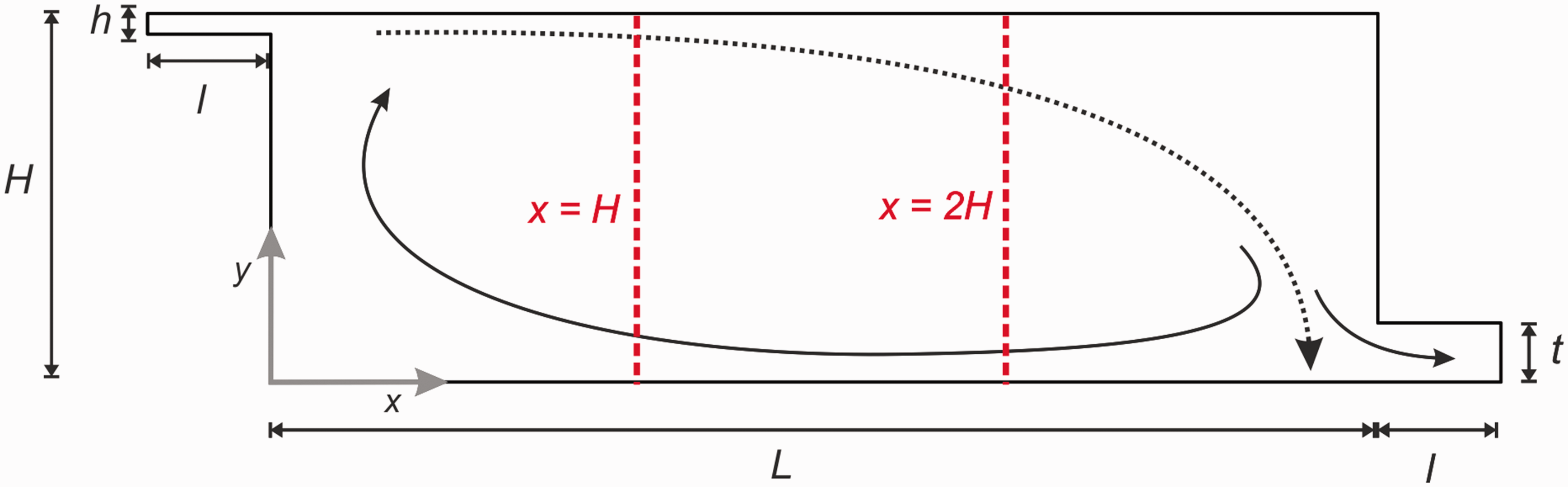
Vertical cross section of room geometry used in the validation study, taken from IEA Annex 20 case, ¹¹ with indication of two vertical lines in vertical centre plane (z/W = 0.5) along which experimental results are compared with numerical results.

The measurements were conducted for Re = 5000, with Re = hU₀/ν, with ν the kinematic viscosity (=15.3 × 10⁻⁶ m²/s at air temperature 20 °C), resulting in a supply velocity of U₀ = 0.455 m/s. The supply condition for turbulent kinetic energy (k₀) was k₀ = 1.5(I_UU₀)², with I_U the streamwise turbulence intensity equal to 4%, while turbulent dissipation rate ε₀ at the supply was calculated from ε₀ = k₀^1.5/l₀, with l₀ = h/10. ¹² The numerical results were compared with measurement results along two vertical lines, at x = H and at x = 2 H, in the vertical centre plane (z/W = 0.5) (Figure 1).

Computational settings and parameters

The computational geometry reproduces the geometry of the model used in the experiments described by Nielsen ¹² (see previous section and Figure 1). The computational grid was created using the surface-grid extrusion technique by van Hooff and Blocken ³⁵ and is presented in Figure 2 (vertical cross section). The computational grid consists of hexahedral cells only. The grid resolution was determined based on a grid-sensitivity analysis using three different grids, which were created by refining and coarsening the basic grid with a factor of √2 in each direction. The resulting coarse, basic and fine grids contain 212,160 cells, 588,672 cells and 1,697,280 cells, respectively. The maximum dimensionless wall distances (y*) along the ceiling (region of highest velocity and thus highest y* values) are 6.4, 3.6 and 2.5, for the coarse, basic and fine grid, respectively. The average y* values along the ceiling are 3.8, 2.6 and 1.6, for the coarse, basic and fine grid, respectively.

Figure 2.

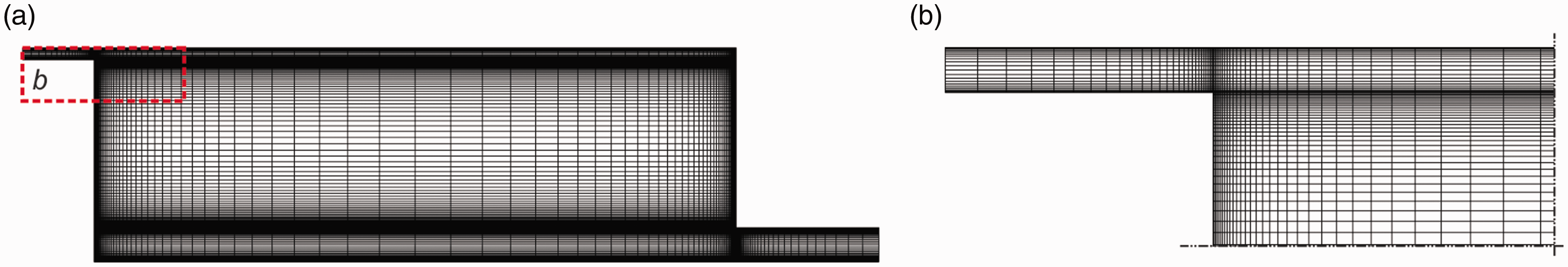
(a) Computational grid in the vertical centre plane (z/W = 0.5) for the validation study (basic grid with 588,672 cells) and (b) Close-up view of grid near the supply opening.

A grid-sensitivity analysis shows that the basic grid provides nearly-grid independent results (see Figure 3). The values of the grid-convergence index (GCI) for the streamwise velocity (U) were calculated using equation (1)

$$\mathrm{G}\mathrm{C}{\mathrm{I}}_{\mathrm{basic}}=F_S\left|\frac{r^p\left[\left({\mathrm{U}}_{\text{basic}}-{\mathrm{U}}_{\mathrm{fine}}\right)/{\mathrm{U}}_0\right]}{1-r^p}\right|$$

(1)

where r is the linear grid refinement factor (r = √2), p the formal order of accuracy which is equal to the value of 2 since second-order discretization schemes were used for the simulations. F_s is a safety factor, taken to be 1.25, which is the recommended value when three or more grids are considered in the grid-sensitivity analysis. ²⁷ Figure 3(c) and (d) shows the results for the GCI. The average GCI values along the two vertical lines (at x = H and x = 2 H) are 0.036 and 0.043, respectively.

Figure 3.

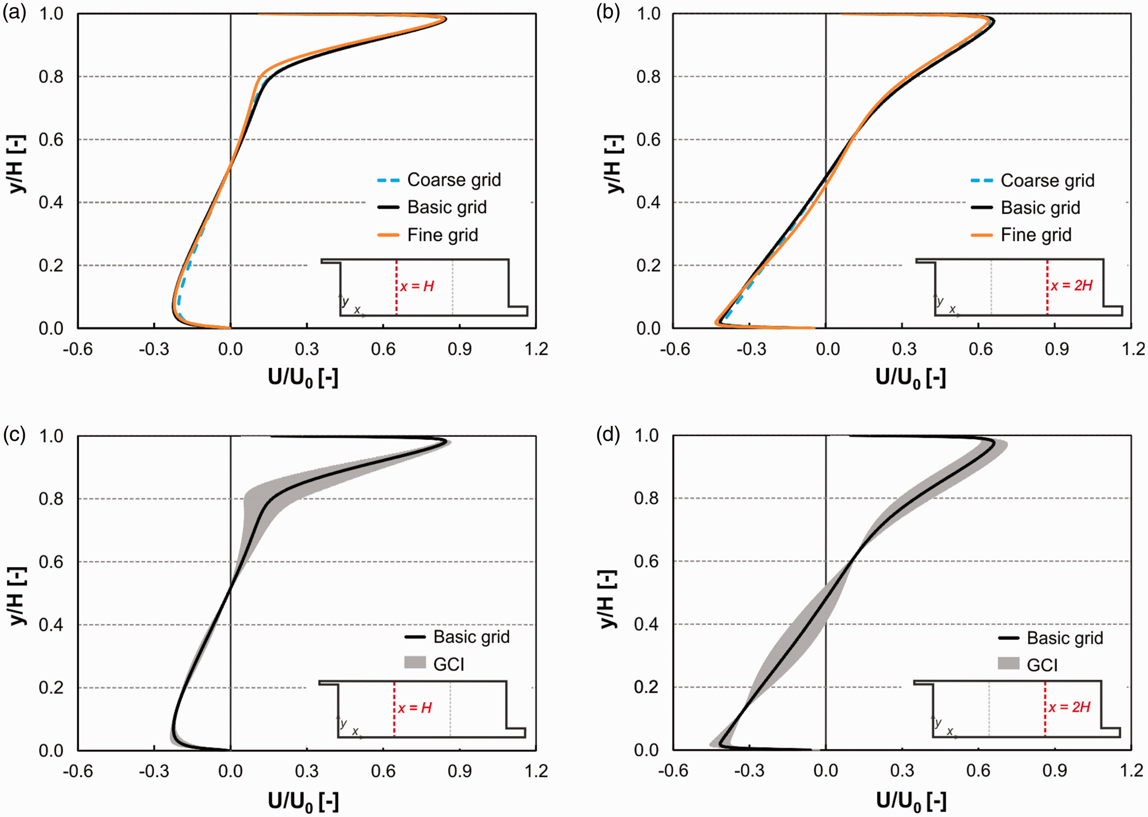
Results of grid-sensitivity analysis. U/U₀ at (a) x = H; (b) x = 2 H. (c) GCI for basic grid at (c) x = H and (d) x = 2 H.

The boundary conditions at the supply and exhaust were taken as equal to those reported by Nielsen ¹² ; i.e. U₀ = 0.455 m/s, ε₀ = k₀^1.5/l₀ = 6.59 10⁻⁴, while the values for k₀ were based on the measured values in the supply opening. ¹² The walls of the enclosure were modelled as no-slip walls, and zero static gauge pressure was applied at the exhaust.

The commercial CFD code ANSYS Fluent 15³⁶ was used for the CFD simulations. The 3D steady RANS equations were solved in combination with the RNG k-ε model ³⁷ and the two-layer zonal model ³⁶ (low Reynolds number modelling) was used as near-wall treatment. The SIMPLE algorithm was used for pressure-velocity coupling, pressure interpolation was second order and second-order discretization schemes were used for both the convective terms and the viscous terms of the governing equations. Convergence was assumed to be obtained when all the scaled residuals level off and reached a minimum value. The minimum values of the residuals are 10⁻⁵ for x, y, z velocities, k, and ε.

Results

Figure 4 shows comparisons between the measured values of the dimensionless time-averaged streamwise velocity (U/U₀) and dimensionless turbulent kinetic energy (k^0.5/U₀) and the values obtained from the 3D steady RANS CFD simulations at x = H and x = 2 H. In general, a good agreement is present along the two vertical lines for U/U₀, with the largest discrepancies near the floor of the enclosure (y/H < 0.3) and the best agreement in the wall jet region (y/H > 0.6), which corresponds to outcomes of earlier validation studies using the same experimental data.^38,39 The values of k^0.5/U₀ are fairly well predicted at x = H (Figure 4(a)); however, at x = 2 H the numerical results show a consistent underprediction of k^0.5/U₀ with about 10–20% (Figure 4(b)). In the lower part of the enclosure (y/H < 0.1), the differences between k^0.5/U₀ obtained from experiments and simulations increase with decreasing height and can become larger than 100% near the ground surface. A possible reason for the higher values of k^0.5/U₀ in the experiments could be the presence of a pronounced transient flow in the region near the floor, which cannot be reproduced by the steady CFD simulations. The observed differences in k^0.5/U₀ could be related to the larger velocity gradients in the lower region in the CFD simulations compared to those in the experiments.

Figure 4.

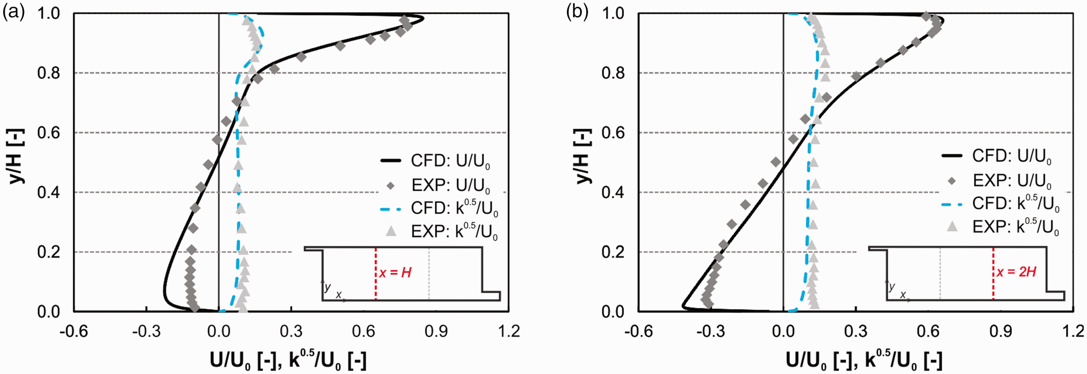
Results of validation study. U/U₀ and k^{0 . 5}/U₀ at (a) x = H and (b) x = 2 H.

Figure 5 shows two scatter plots with the CFD results and the experimental results. A perfect agreement would mean the symbols are on the x = y line. The dashed lines indicate the 10%, 20% and 30% (in case of k^0.5/U₀) difference between the experimental results and the CFD results. Figure 5(a) shows that the largest percentage differences occur in the low-velocity regions and that the best agreement is present in the high-velocity regions. The majority of the predicted velocities lies within 20% difference of the experimental results. Figure 5(b) shows an underprediction of k^0.5/U₀ by the CFD simulations. A bit more than half of the predictions are within 20% difference, and more than 80% of the predictions are within a 30% difference.

Figure 5.

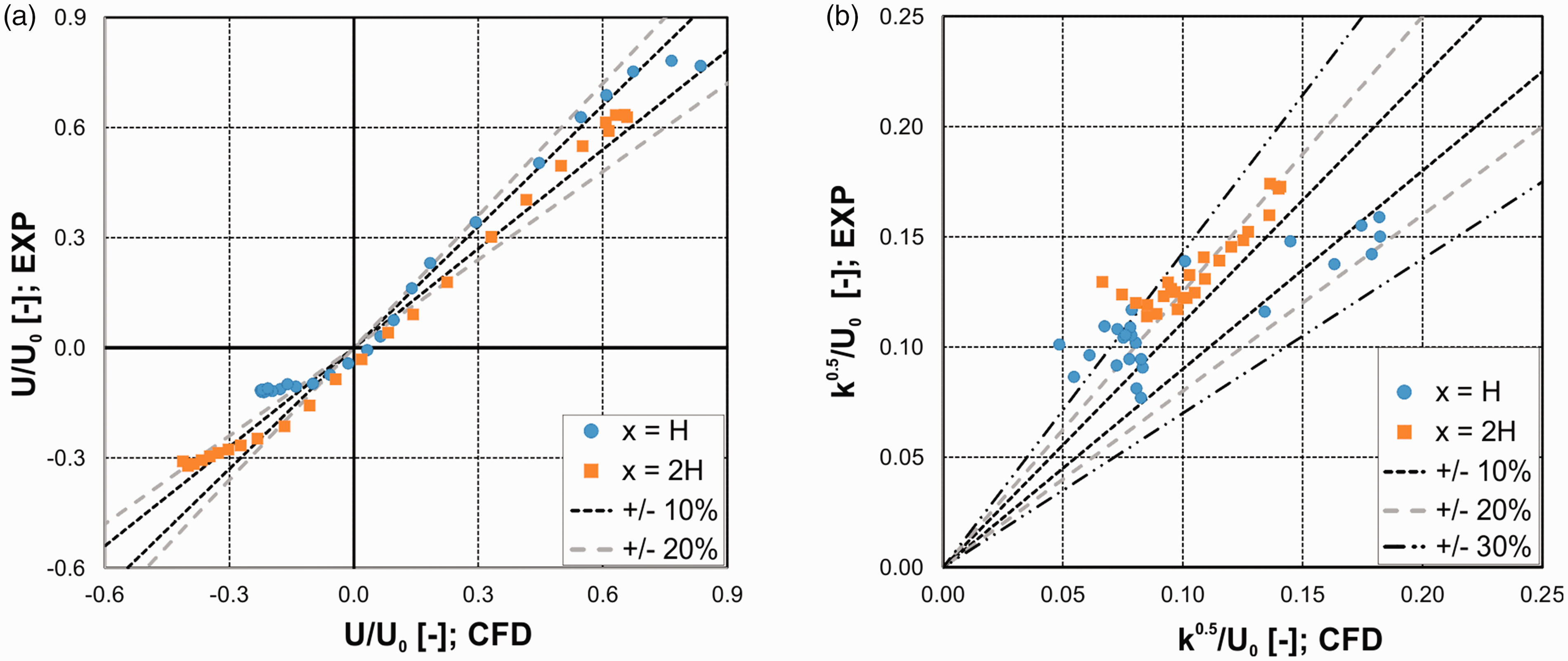
Scatterplot with results of validation study at x = H and x = 2 H. (a) U/U₀ and (b) k^0.5/U₀.

Overall, the validation study shows that the RNG k-ε turbulence model in combination with the other employed computational settings and parameters is sufficiently capable of predicting mixing ventilation flows in a generic enclosure with sufficient accuracy, especially with respect to the mean velocities. Therefore, the employed turbulence model and settings are used in the case study in the following section.

Case study: Computational geometry, settings and parameters

Computational geometry

The effect of time-periodic forcing of the supply velocity on the mixing ventilation flow was assessed in a generic rectangular enclosure based on the IEA Annex 20 enclosure as presented in the Validation study section, with dimensions 9 × 3 × 3 m³ (L × W × H). ¹² However, in this case, the air was supplied by two oppositely located linear supply openings (h_supply = 0.168 m, l_supply is 3 m) in the upper part of the enclosure and it leaves the enclosure through two oppositely located linear exhausts (h_exhaust = 0.48 m, l_supply is 3 m) in the bottom part of the enclosure (see Figure 6). The results were analysed in the vertical centre plane (z/W = 0.5) along three vertical lines (x/H = 1/3, x/H = 2/3, x/H = 1; Figure 6).

Figure 6.

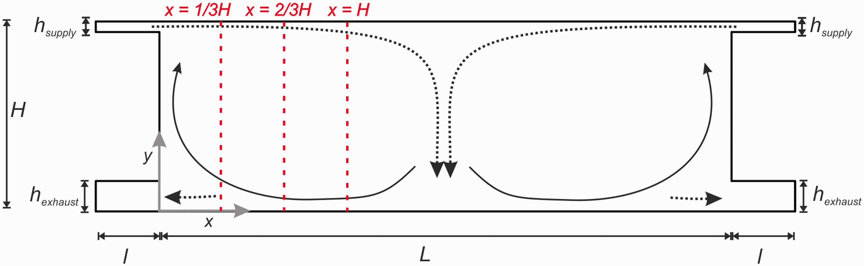
Vertical cross section of room geometry, with two opposite supply openings in the upper part and two opposite exhaust openings in the lower part of the enclosure. The three dashed vertical lines indicate the locations where the results were analysed.

Computational settings and parameters

The 3D CFD simulations were performed in ANSYS Fluent. ³⁶ A vertical cross section of the computational geometry is depicted in Figure 6, including indication of the coordinate system. The computational grid was based on the grid resolution employed in the validation study and consists of 505,760 hexahedral cells, with higher grid resolutions in the boundary layer, shear layer and in the region where the two opposite jets collide/interact in case of constant supply velocities (see Figure 7).

Figure 7.

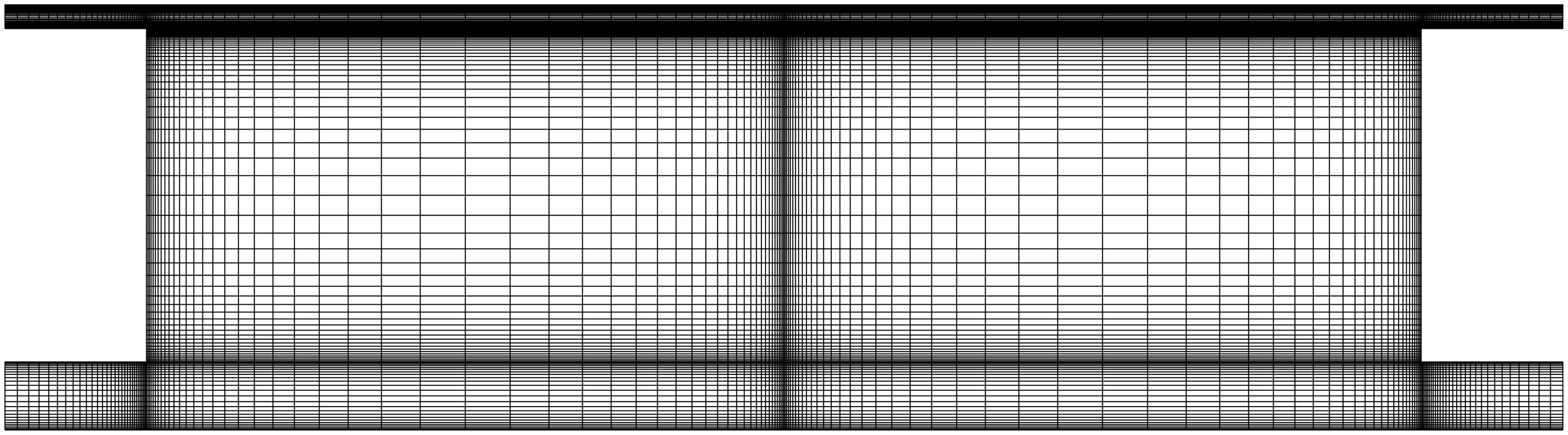
Computational grid for the case study (505,760 hexahedral cells).

One type of time-periodic supply velocity was used in the present paper, which was based on a sine function. The sine function enables a supply velocity that varies over time t with period T and amplitude ΔU₀ around a constant reference velocity U_0,RC (= 0.5 m/s) and is described by equation (2) (supply 1) and equation (3) (supply 2):

$$u_0{\hspace{0.17em}}_{\text{,supply1}}\left(t\right)={\mathrm{U}}_{0,RC}+\Delta {\mathrm{U}}_0\cdot \sin \left(2\pi t/\mathrm{T}\right)$$

(2)

$$u_0{\hspace{0.17em}}_{\text{,supply2}}\left(t\right)=-\left({\mathrm{U}}_{0,RC}-\Delta {\mathrm{U}}_0\cdot \sin \left(2\pi t/\mathrm{T}\right)\right)$$

(3)

The first case, as reported before, has a period of T = 0.2τ_n, with τ_n the nominal time constant, which is the shortest possible time to replace the air in an enclosure (τ_n = V_enclosure/Q, with V_enclosure the volume of the enclosure and Q the volume flow rate supplied), which is equal to 161 s for the chosen supply velocity of U_0,RC = 0.5 m/s and the geometry used. In the next section, the influence of the chosen period was assessed using three different periods, equal to T = 0.1τ_n, T = 0.2τ_n (see Figure 8) and T = 0.4τ_n. In the reference case, the supply velocity at both supply openings is constant. i.e. U_0,RC = 0.5 m/s and the amplitude was fixed at ΔU₀ = 0.5 m/s. The different sine functions were imposed with a user-defined function (UDF) in Fluent. At the supply openings, a turbulence intensity was imposed of 10% in combination with a turbulent viscosity ratio of μ_t/μ = 10. Zero static gauge pressure was imposed at the exhausts. A passive uniformly distributed pollutant source (C_s = 10⁻⁶kg/m³s) was imposed throughout the entire 3D volume of the enclosure in order to be able to assess the ventilation efficiency, i.e. this pollutant source was imposed as a source term in the entire fluid volume in Fluent.

Figure 8.

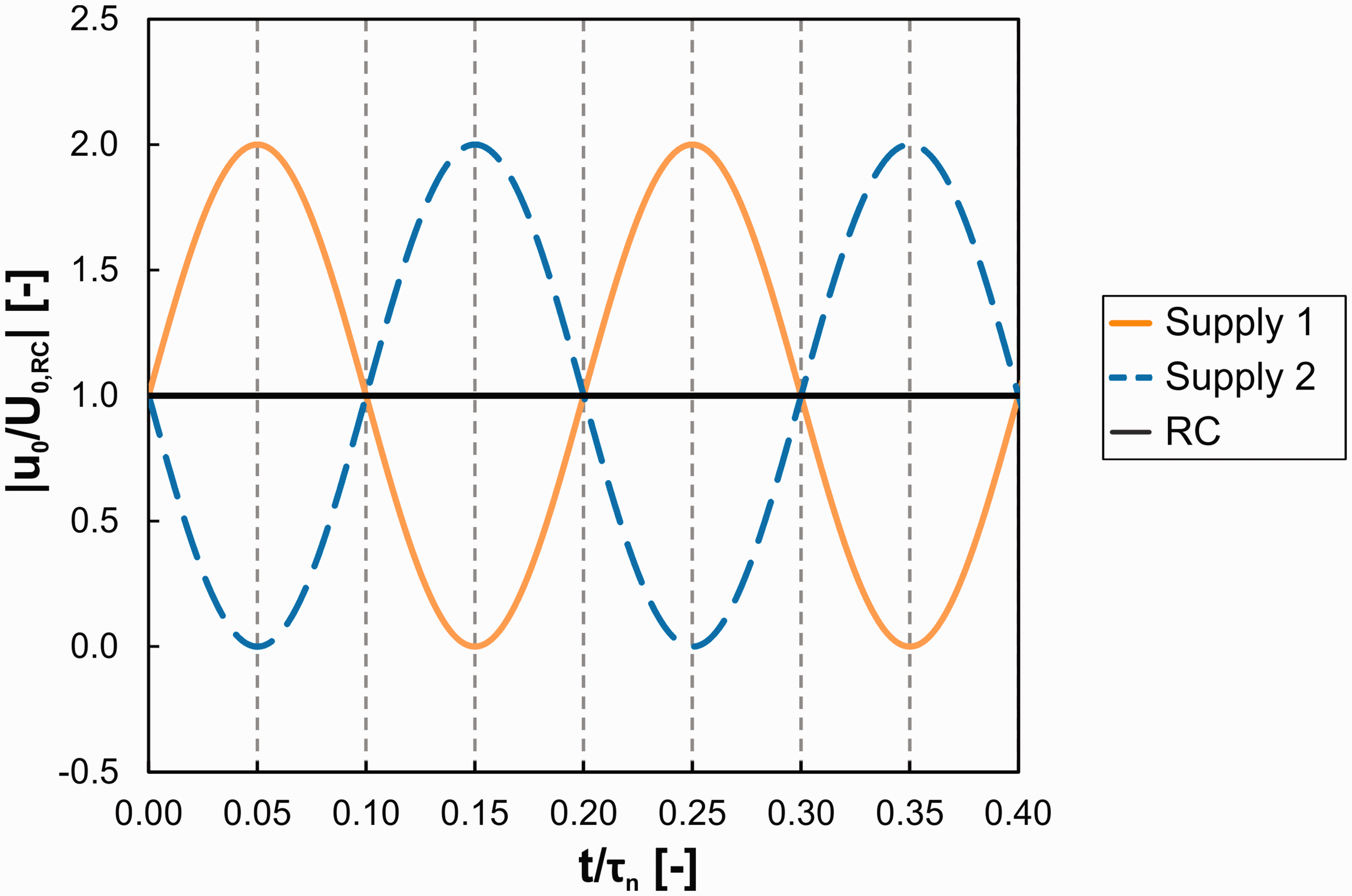
Absolute values of x-velocity component for the two opposite jets (T = 0.2τ_n) as a function of time and the constant dimensionless supply velocity for the reference case (RC; equal velocity at both supplies).

The RNG k-ε turbulence model ³⁷ was employed for the URANS simulations, in which discretization schemes and pressure interpolation are second order, and the SIMPLE algorithm was used for pressure–velocity coupling. Pollutant concentrations were obtained using an advection–diffusion equation (Eulerian approach); turbulent mass transport was calculated using the standard-gradient diffusion hypothesis. The turbulent Schmidt number (Sc_t), which relates the turbulent viscosity to the turbulent mass diffusivity as present in the standard gradient-diffusion hypothesis (D_t = ν_t/Sc_t), was set to 0.7. The time integration was bounded second-order implicit. The time step Δt = 0.1 s in the URANS simulation for T = 0.2τ_n was based on a sensitivity analysis using time-step sizes of Δt = 1 s, Δt = 0.1 s and Δt = 0.01 s. Note that the time-step size was halved and doubled for T = 0.1τ_n and T = 0.4τ_n, respectively. The number of iterations within one time-step was equal to 10 and it was verified that both the number of iterations and the averaging time are sufficient (i.e. > 100 periods) by monitoring the evolution of the instantaneous (within a time-step) and time-averaged (over number of time-steps) velocities and pollutant concentrations.

Case study: Results

Constant supply vs. time-periodic supply

Figure 9 compares the dimensionless time-averaged velocity magnitude |V|/U_0,RC, with |V| denoting the magnitude of the time-averaged velocity vector, obtained from the reference case with constant supply velocities and from the case with time-periodic supply velocities with a period of T = 0.2τ_n. Here, U_0,RC is the value at supply opening 1 in the reference case, i.e. 0.5 m/s. Figure 9 shows that along all three vertical lines (x/H = 1/3, x/H = 2/3, x/H = 1) |V|/U_0,RC is higher in the time-periodic case than in the reference case, with the smallest average difference over the height at x/H = 1/3 (0.13) and the largest average difference over the height at x/H = 1 (0.22). At location x/H = 1, the reference case exhibits larger velocity gradients in the upper part of the enclosure (y/H > 0.8), due to the distinct presence of a constant incoming wall jet resulting in a clear shear layer, while the time-periodic cases result in a more uniform distribution of velocities with height due to the enhanced mixing driven by the time-periodic supply velocity. The velocities along all three lines are generally higher due to the higher supply kinetic energy levels for equal time-averaged velocities. A more detailed analysis on the influence of the supply kinetic energy levels is provided later.

Figure 9.

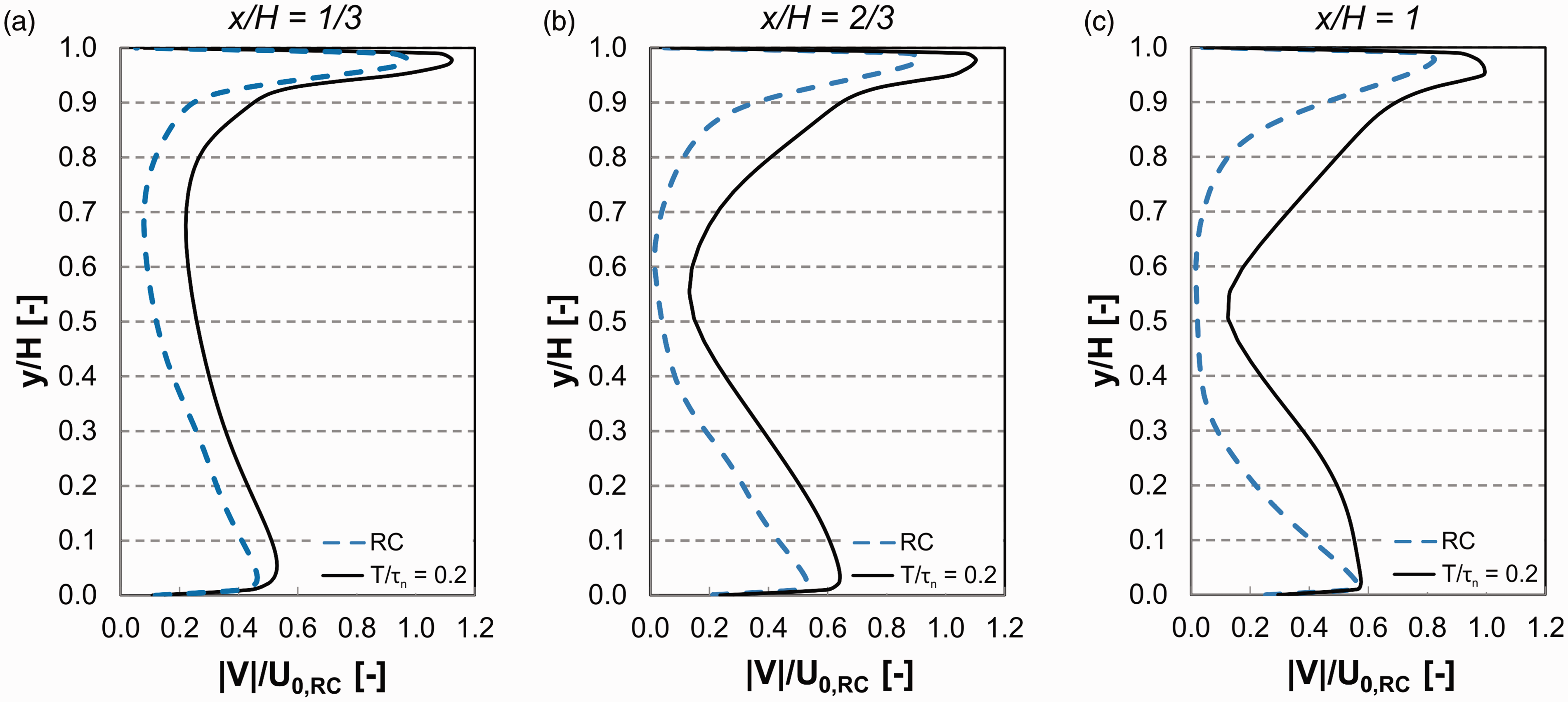
|V|/U_{0 ,RC} along three vertical lines in the vertical centre plane (z/W = 0.5). (a) x/H = 1/3. (b) x/H = 2/3 and (c) x/H = 1. Results for reference case (RC) and time-periodic supply case (T = 0.2τ_n).

Figure 10 shows contours of |V|/U_0,RC in the vertical centre plane. The stagnant (blue) regions as present in Figure 10(a) for the reference case have decreased due to the time-periodic supply velocities as shown in Figure 10(b). In general, the time-averaged velocities are higher, which is also reflected in the volume-averaged dimensionless time-average velocity, which is 0.258 in the reference case versus 0.399 for the case with time-periodic supply velocities. These results also indicate the influence of higher supply kinetic energy levels resulting from the higher maximum velocities due to the use of a sine function for the supply velocities.

Figure 10.

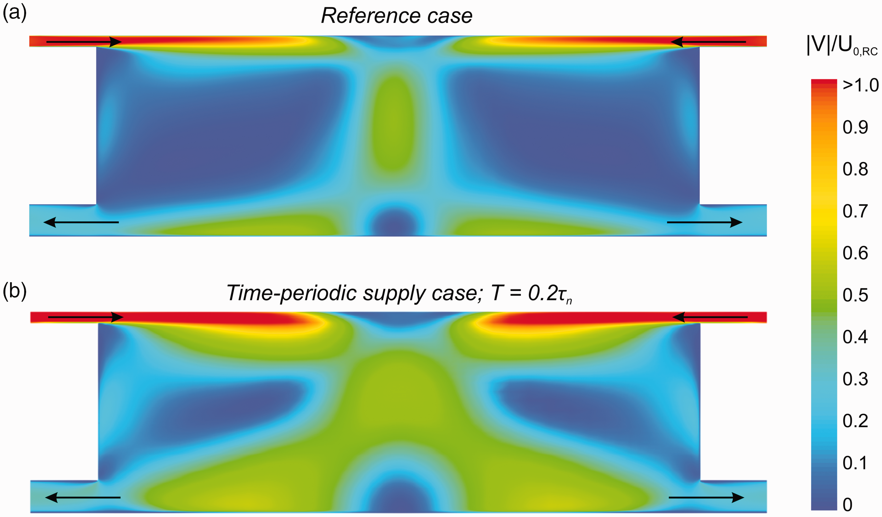
Contours of |V|/U_{0 ,RC} in vertical centre plane (z/W = 0.5). (a) Reference case and (b) Time-periodic supply case (T = 0.2τ_n).

Figure 11 shows a comparison between the dimensionless time-averaged pollutant concentrations (Cρ/C_sτ_n) obtained from the reference case with steady supply velocities versus the case with time-periodic supply velocities with a period of T = 0.2τ_n. The largest differences (up to 74%; 1.455 vs. 0.834) occur around mid-height of the enclosure (0.5 < y/L < 0.6) at x/H = 2/3 and x/H = 1, where in the reference case high pollutant concentrations are present due to a stagnant region. In the case of time-periodic supply velocities the pollutant concentrations in this area are strongly reduced. In addition, the pollutant concentration along all three vertical lines (below y/H = 0.9) are around 1 and are thus similar throughout large parts of the domain, indicating enhanced mixing and the resulting more uniform concentrations.

Figure 11.

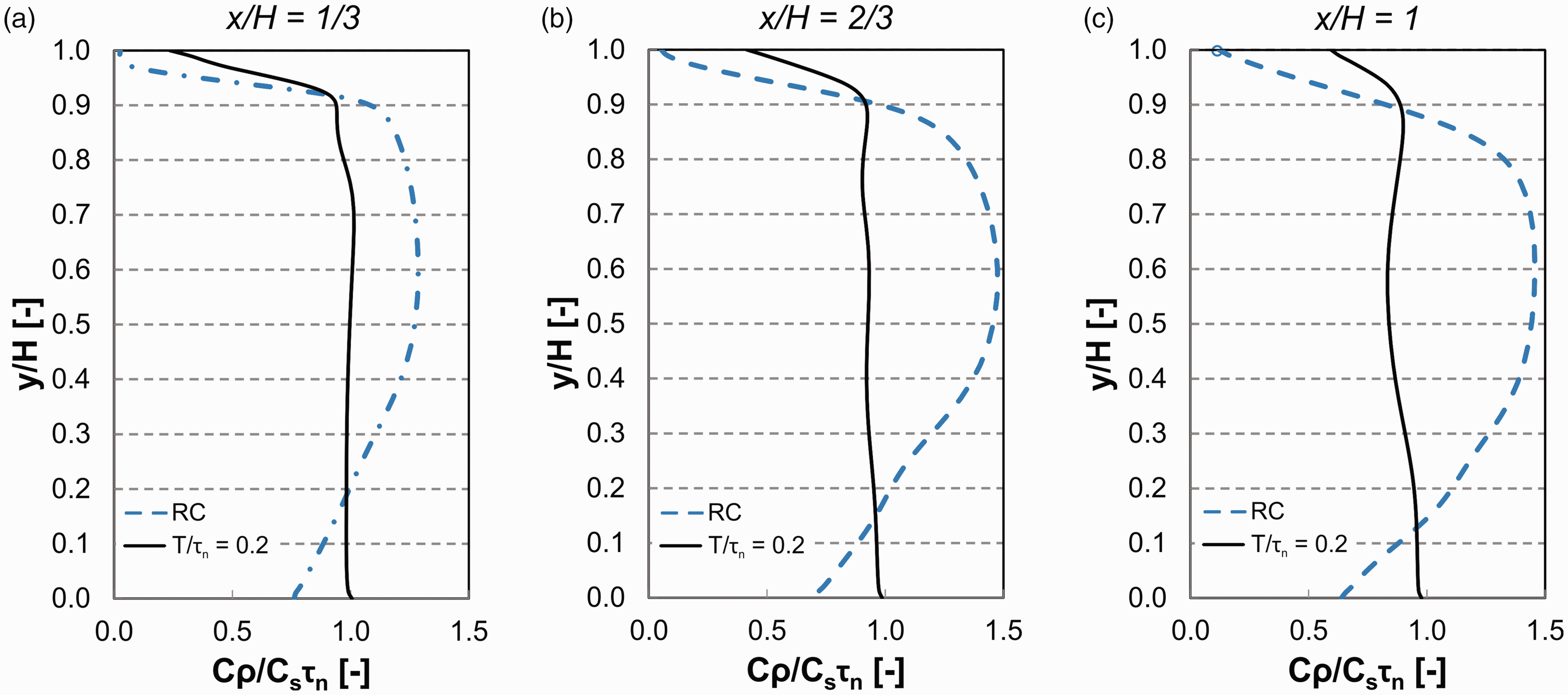
Cρ/C_sτ_n along three vertical lines in the vertical centre plane (z/W = 0.5). (a) x/H = 1/3. (b) x/H = 2/3 and (c) x/H = 1. Results for reference case (RC) and time-periodic supply case (T = 0.2τ_n).

Figure 12 shows the time-averaged pollutant concentrations in the enclosure for both cases. Time-periodic supply velocities lead to substantially reduced concentration. The improved mixing leads to the absence of high pollutant concentration regions and the relatively uniform distribution of pollutant concentrations.

Figure 12.

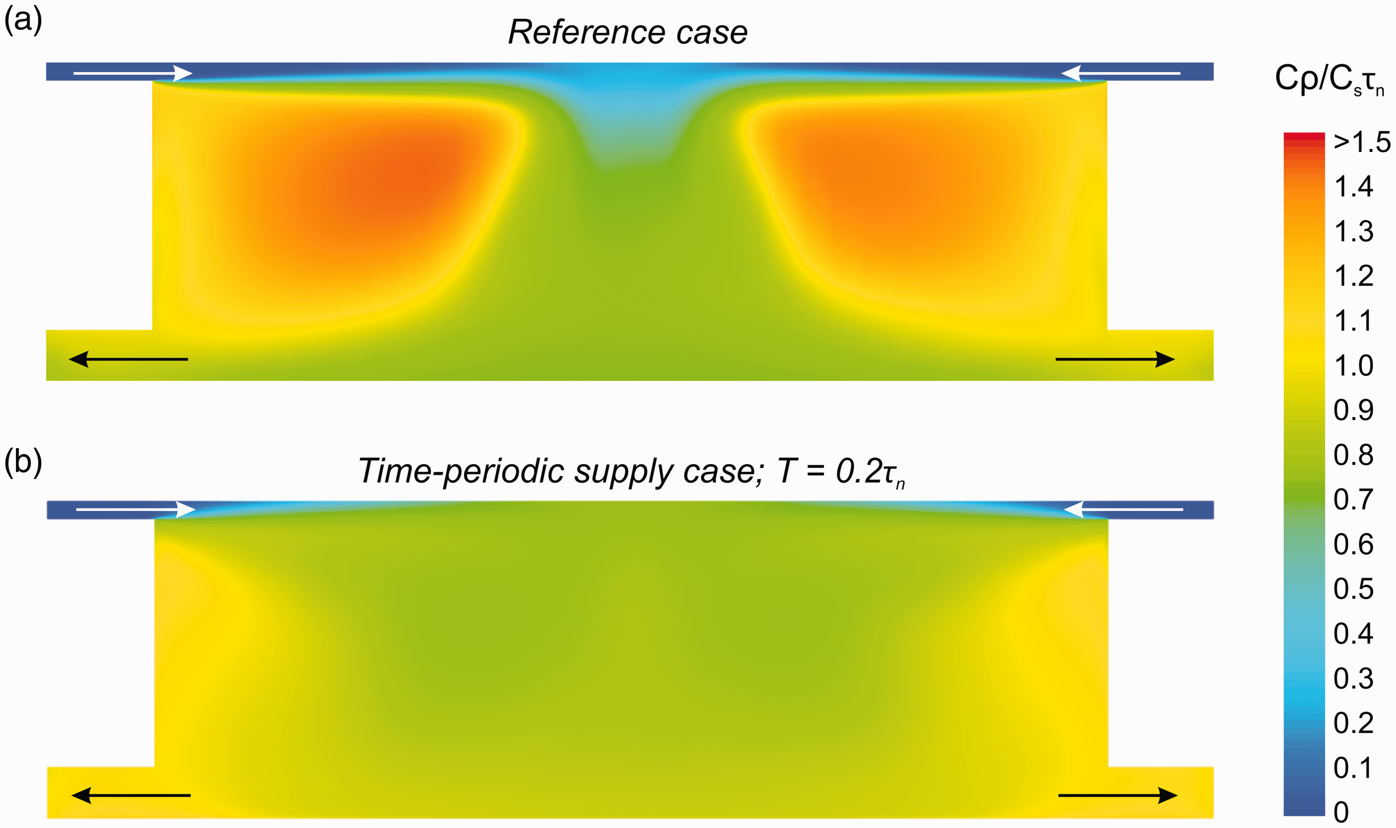
Contours of Cρ/C_sτ_n in the vertical centre plane (z/W = 0.5). (a) Reference case and (b) Time-periodic supply case (T = 0.2τ_n).

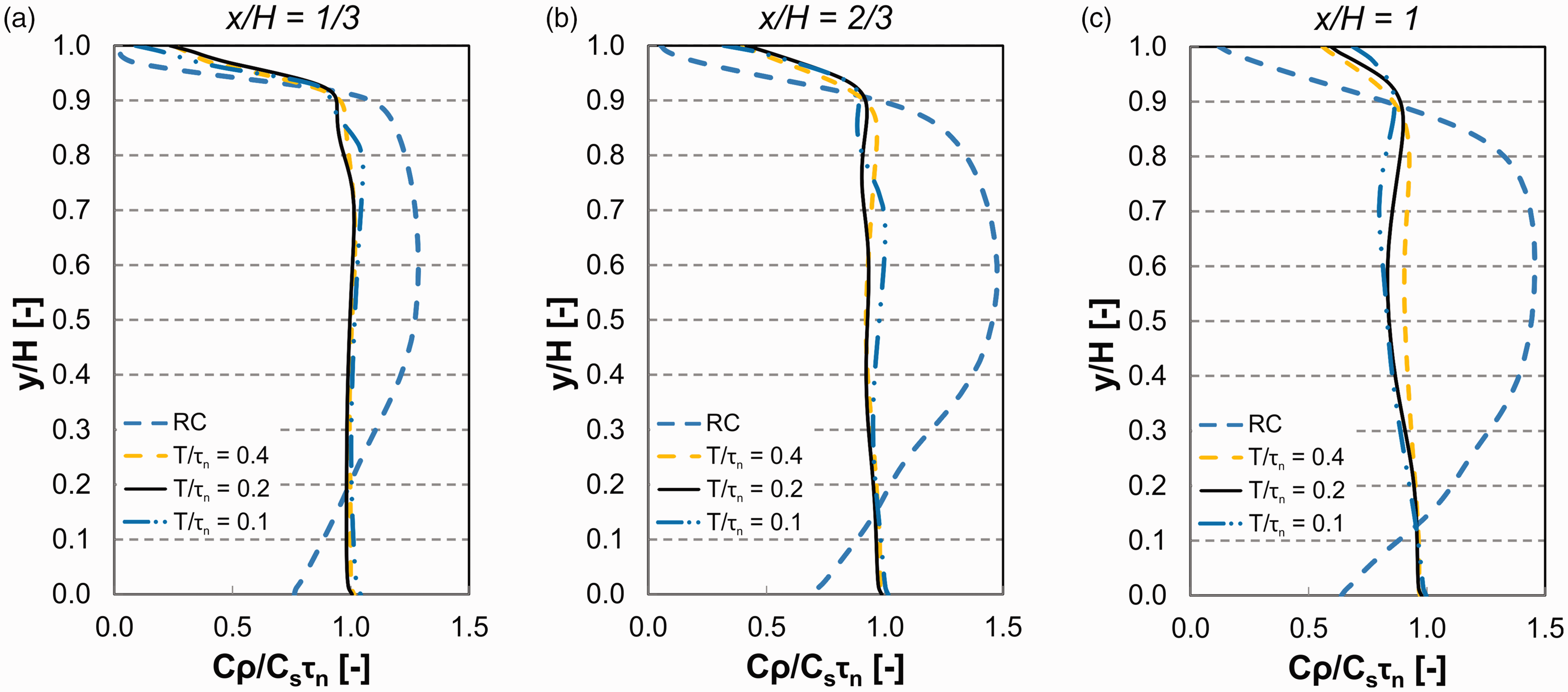
The volume-averaged value for the reference case is Cρ/C_sτ_n = 1.018 versus 0.908 for the time-periodic supply case. At the exhaust openings the area average value is 0.976 for the reference case versus 1.050 for the time-periodic supply case. The CRE (ε_C)^40,41 can be calculated using equation (4), using the room-averaged time-averaged pollutant concentration (⟨C⟩), the time-averaged pollutant concentration at the supply (C_s), and the time-averaged pollutant concentration at the exhaust (C_e)

$${\epsilon }_C=\frac{{\mathrm{C}}_{\mathrm{e}}-{\mathrm{C}}_{\mathrm{s}}}{〈\mathrm{C}〉-{\mathrm{C}}_{\mathrm{s}}}\cdot 100\%$$

(4)

Fully mixed conditions would result in a value of 100%, piston flow would result in a value equal to or greater than 100% (depending on location of pollutant source), and short-circuiting would result in values below 100% (room averaged concentration would be larger than concentration at exhaust).^40,41 The CRE is equal to ε_C = 96% for the reference case, while it is 116% for the case with time-periodic supply velocities.

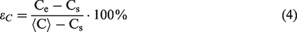
Finally, Figure 13 depicts contours of instantaneous pollutant concentrations for the case with a period of T = 0.2τ_n, during one period (T) starting after time-averaged values are obtained (i.e. after > 100 periods). Figure 13 shows the back and forth movement of the flow in the enclosure as driven by the wall jets and the breakup of the recirculation cells. In the reference case two distinct recirculation cells are visible (Figure 12(a)), with stagnant regions in the middle of each recirculation cell resulting in higher pollutant concentrations in these regions. Note that no symmetric flow can be observed during this period due to the 3D nature of the flow, with randomly varying pollutant concentrations over the width of the enclosure (not shown here for the sake of brevity).

Figure 13.

Contours of dimensionless instantaneous pollutant concentration (cρ/C_sτ_n) in the vertical centre plane (z/W = 0.5) during one period T for T = 0.2τ_n.

Influence of period

The influence of the chosen period was analysed by simulations with three different periods, i.e. T = 0.1τ_n, T = 0.2τ_n, and T = 0.4τ_n. The amplitude was kept constant. The time-averaged supply velocity (and thus supply volume flow rate) is constant (= 0.5 m/s) in all three cases.

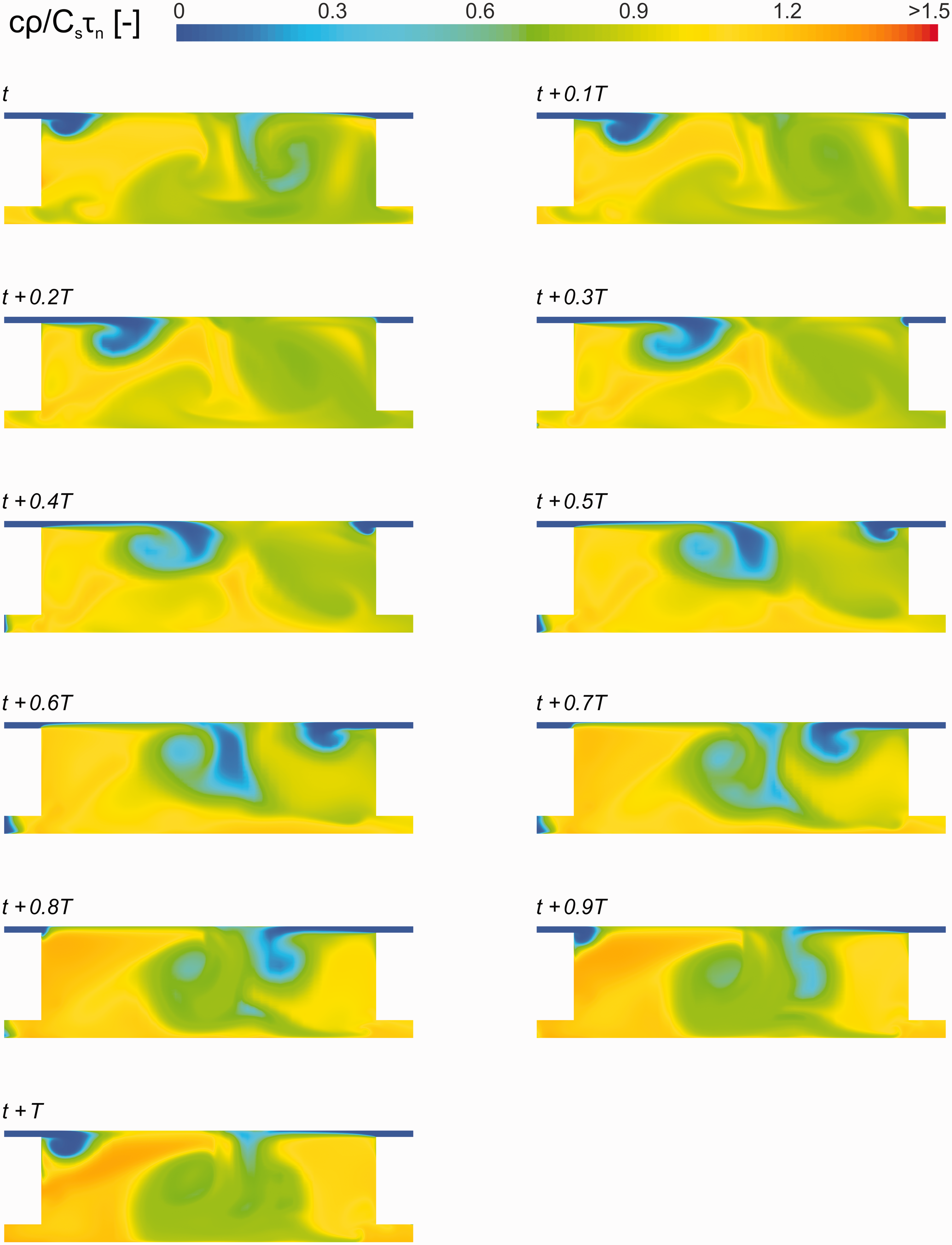
Figure 14 compares the dimensionless time-averaged velocities from the reference case versus the cases with time-periodic supply velocities with the three different periods. The influence of the period appears to be limited, especially at x/H = 2/3 and x/H = 1. At x/H = 1/3 the largest differences are present; the velocity profile for a period of T = 0.1τ_n differs from the other two velocity profiles. Nonetheless, Figure 14 shows that the overall differences in velocity magnitude along the three vertical lines is limited.

Figure 14.

Influence of period. |V|/U_{0 ,RC} along three vertical lines in the vertical centre plane (z/W = 0.5). (a) x/H = 1/3. (b) x/H = 2/3 and (c) x/H = 1.

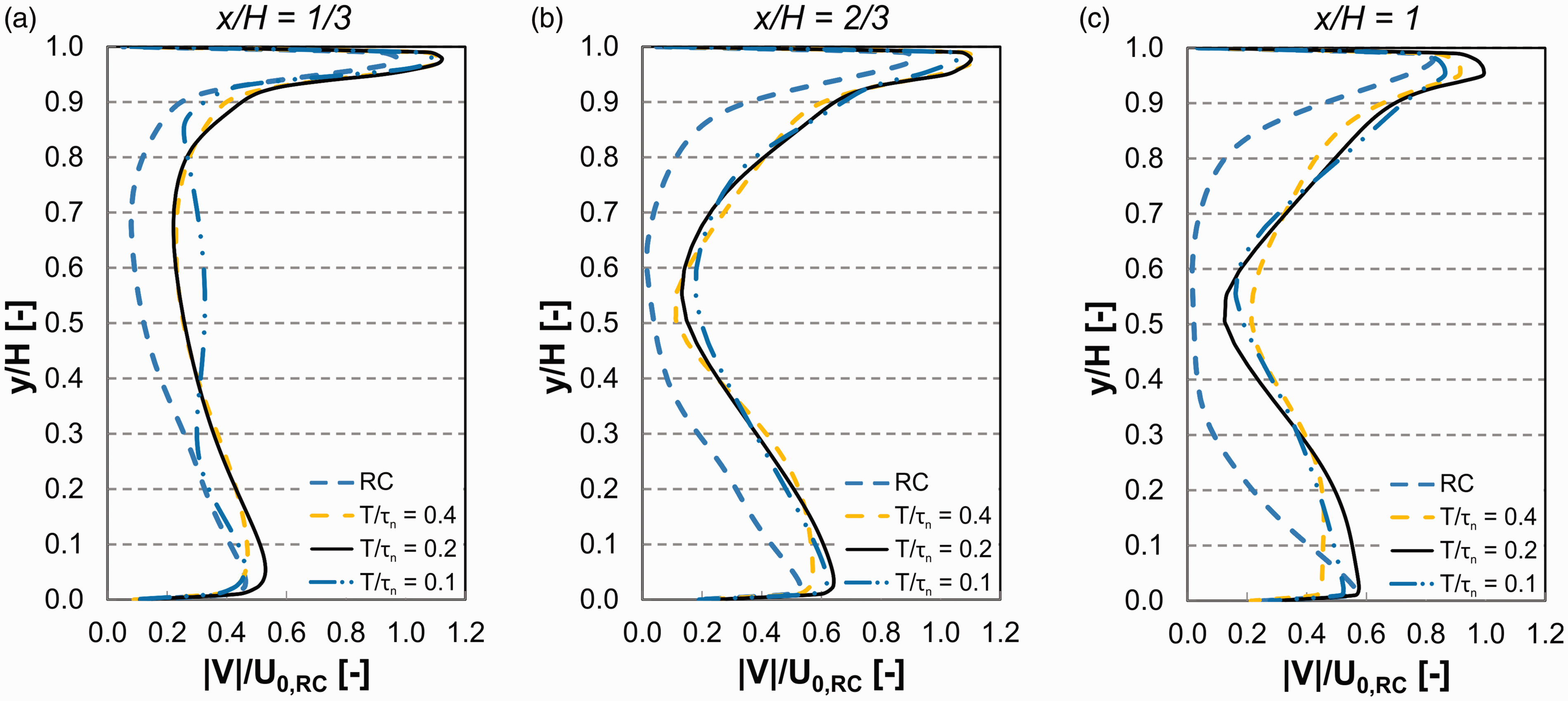
Figure 15 compares the dimensionless time-averaged pollutant concentrations along the same three lines. The difference between the different periods appears to be marginal along the lines analysed. The average difference between the time-averaged pollutant concentrations over the three lines was within 1.3%, while the maximum differences were within 10%. This indicates that the periods tested do not significantly influence the mixing and thus the resulting time-averaged pollutant concentrations, for this particular case.

Figure 15.

Influence of period. Cρ/C_sτ_n along three vertical lines in the vertical centre plane (z/W = 0.5). (a) x/H = 1/3. (b) x/H = 2/3 and (c) x/H = 1.

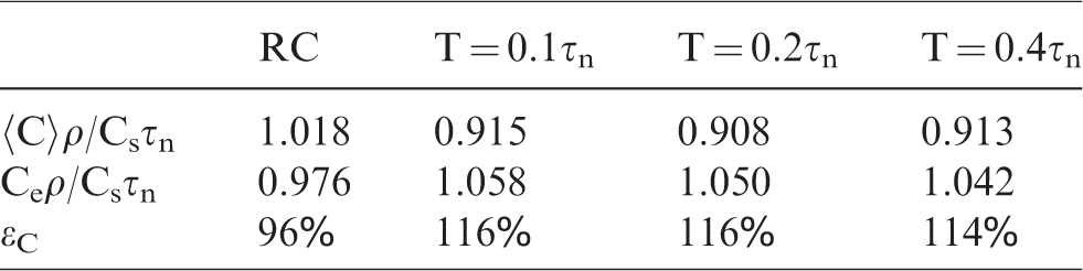
The volume-averaged (whole enclosure) and surface-averaged (over area of exhausts) values of Cρ/C_sτ_n and the CRE for the reference case and the three cases with time-periodic supply velocities are listed in Table 1. The values for the cases with a time-periodic supply but different periods are very similar, with ε_C = 116% for T = 0.1τ_n and T = 0.2τ_nv, versus ε_C = 114% for T = 0.4τ_n.

Table 1.

Influence of period on dimensionless time-averaged pollutant concentrations, averaged over the volume (⟨C⟩ρ/C_sτ_n) and averaged over the exhaust opening (C_eρ/C_sτ_n), and CRE (ε_C).

	RC	T = 0.1τn	T = 0.2τn	T = 0.4τn
⟨C⟩ρ/Csτn	1.018	0.915	0.908	0.913
Ceρ/Csτn	0.976	1.058	1.050	1.042
εC	96%	116%	116%	114%

Equal supply volume flow rates vs. equal supply kinetic energy levels

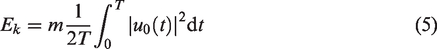
In the simulations reported in the previous sections, the time-averaged supply velocity (and thus supply volume flow rate) was taken equal in the reference case and in all three time-periodic supply cases. Although this choice can be substantiated from the point of view of heating and cooling demands (the energy needed to heat or cool a certain amount of air would be different when different supply volume flow rates would be used), considering fan energy use, however, one should use the same time-averaged supply kinetic energy values for the reference case compared to the time-periodic supply velocity cases. Therefore, an additional simulation was conducted in which the time-averaged supply kinetic energy for all cases is equal, which was achieved by increasing the supply velocity at both supplies in the reference case to 0.61 m/s, based on equation (5)

$$E_k=m\frac{1}{2T}{\displaystyle {\int }_0^T{\left|u_0(t)\right|}^2\text{d}t}$$

(5)

with u₀(t) being the supply velocity and m is the mass of air (equal in both cases). Figures 16 and 17 compare the results focused on equal time-averaged supply volume flow rates versus equal time-averaged levels of kinetic energy of the supply flow. Figure 16 shows that the time-averaged velocities along the three vertical lines are slightly higher due to the higher supply velocity (0.61 m/s vs. 0.5 m/s) imposed for the reference case with equal time-averaged supply kinetic energy levels (RC_KE). The increase is most pronounced in the wall jet region (y/H > 0.9). The volume-averaged dimensionless time-average velocity, which is 0.258 in the reference case with equal time-averaged supply volume flow rates (RC) versus 0.363 for the reference case with equal time-averaged kinetic energy of the supply flow (RC_KE), and 0.399 for the case with time-periodic supply velocities.

Figure 16.

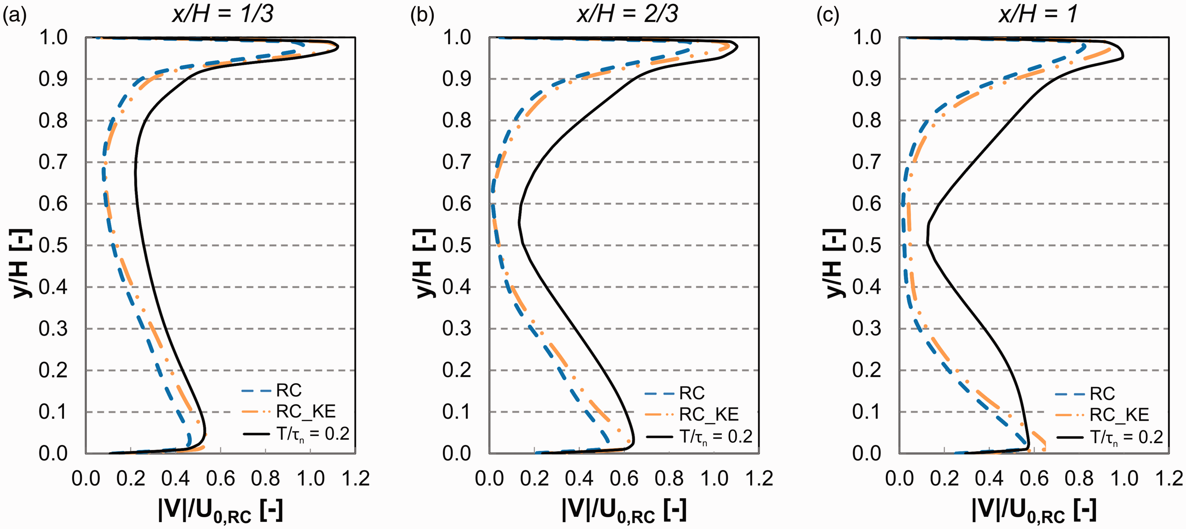
|V|/U_{0 ,RC} along three vertical lines in the vertical centre plane (z/W = 0.5). (a) x/H = 1/3. (b) x/H = 2/3 and (c) x/H = 1. For RC with time-averaged supply volume flow rates equal to time-periodic case (RC) and RC with time-averaged kinetic energy of supply flow equal to time-periodic case (RC_KE).

Figure 17.

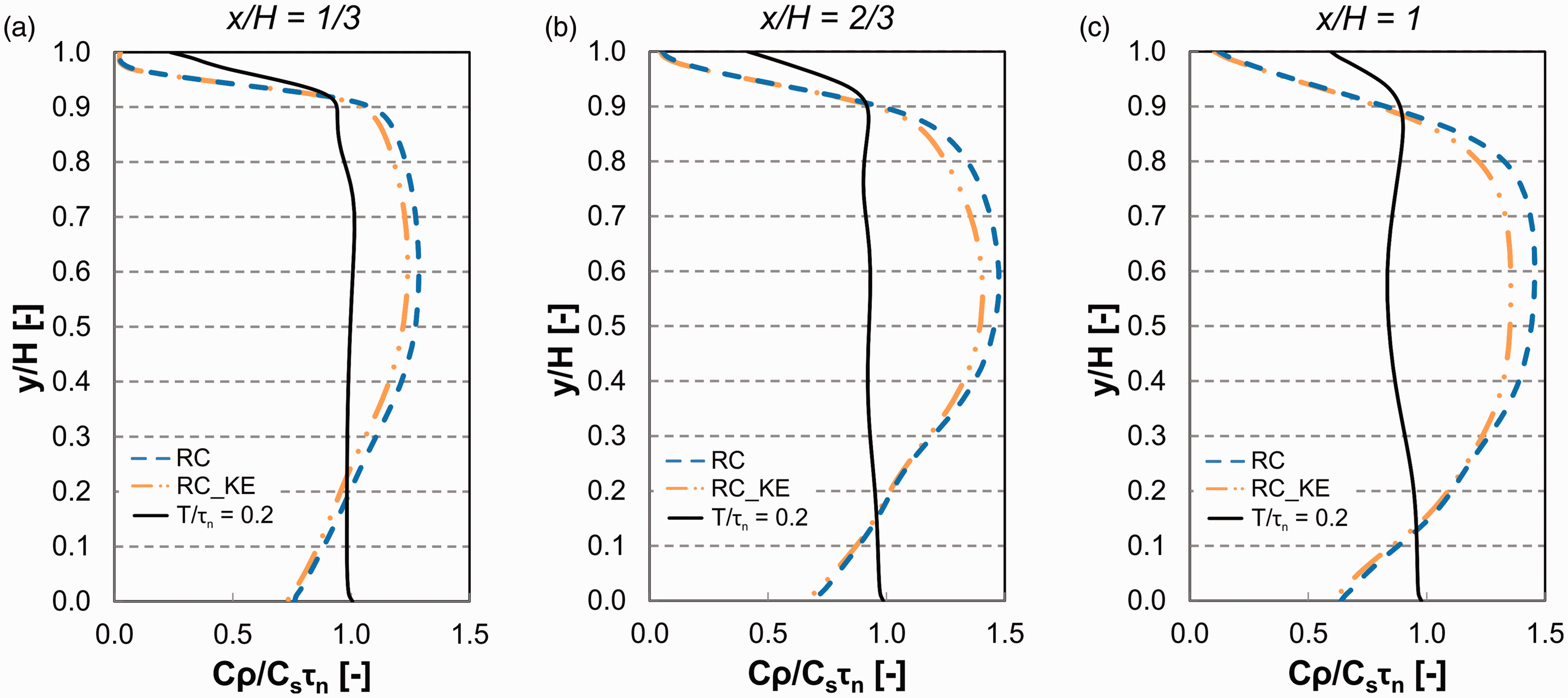
Cρ/C_sτ_n along three vertical lines in the vertical centre plane (z/W = 0.5). (a) x/H = 1/3. (b) x/H = 2/3 and (c) x/H = 1. For RC with time-averaged supply volume flow rates equal to time-periodic case (RC) and RC with time-averaged kinetic energy of supply flow equal to time-periodic case (RC_KE).

Figure 17 shows that the pollutant concentrations in RC_KE have decreased to a certain extent compared to RC, however, the pollutant concentrations in both reference cases are still much higher at mid-height than in the time-periodic supply case. The maximum decrease of Cρ/C_sτ_n for RC_KE compared to RC is around 8% at x/H = 1 and y/H ≈ 0.7. The time-averaged values of both the volume-averaged pollutant concentrations (⟨C⟩ρ/C_sτ_n) and the surface-averaged pollutant concentration at the exhaust opening (C_eρ/C_sτ_n), and the CRE are listed in Table 2. Although the value for ⟨C⟩ρ/C_sτ_n is about 10% lower for RC_KE compared to RC, it is still 1.5% higher for RC_KE than for the time-periodic supply case. Moreover, the CRE for RC_KE is very similar (95%) to the one for RC (96%) and thus much lower than the CRE in the time-periodic supply case (116%). The increased velocity in RC_KE thus decreases the volume-averaged time-average pollutant concentration compared to RC but has no significant effect on the CRE. The results indicate that the CRE in both reference cases is much lower than in the time-periodic case, implying that at equal kinetic energy levels of the supply flow (and thus equal fan energy) time-periodic ventilation can enhance mixing and the CRE. The volume-averaged pollutant concentration for the time-periodic supply case is 1.5% lower than in RC_KE, and this decrease could be achieved with equal energy use. Note that any possible changes in fan efficiency as function of supply volume flow rate are not included here.

Table 2.

Comparison of dimensionless time-averaged pollutant concentrations, averaged over the volume (⟨C⟩ρ/C_sτ_n) and averaged over the exhaust opening (C_eρ/C_sτ_n), and CRE for RC and RC_KE with T = 0.2τ_n.

	RC	RC_KE	T = 0.2τn
⟨C⟩ρ/Csτn	1.018	0.922	0.908
Ceρ/Csτn	0.976	0.877	1.050
CRE (%)	96	95	116

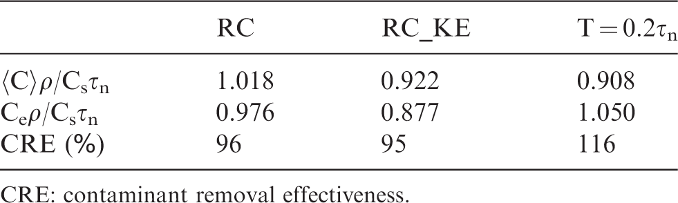
CRE: contaminant removal effectiveness.

URANS vs. LES

To ascertain the suitability of URANS simulations to capture the effect of time-periodic supply velocities on the mixing ventilation flow, additional simulations were conducted using the LES approach. LES is intrinsically more accurate when applied according to best-practice guidelines since the larger scales of turbulence (larger than the filter applied, which is often the grid size) are resolved instead of modelled, as is the case in URANS. However, LES significantly increases the computational demand (increase with about 10² (e.g. Chen ²³ )) and is thus less suitable for an exploration of the proposed new concept of time-periodic supply velocities, since a large number of parameters are to be studied (e.g. period, amplitude, mean velocity, room geometry, ventilation configuration). In fact, for several applications of building simulation for outdoor and indoor environments, it has been shown that RANS is accurate enough and that one should not always resort to LES. ⁴² The LES simulations in the present papers were conducted on the same grid as the URANS simulations. The dynamic Smagorinsky subgrid-scale model^43–45 was used and the filtered momentum equations were discretized with a bounded central-differencing scheme. A second-order upwind scheme was used for the advection-diffusion equation. Pressure interpolation is second order. Time integration is bounded second-order implicit. Pressure–velocity coupling was taken care of by the PISO algorithm. The non-iterative time advancement scheme was used. The time step Δt was based on a maximum CFL number of 1 and is equal to Δt = 0.01 s. The averaging time was verified as sufficient to obtain statistically-steady results by monitoring the evolution of the time-averaged velocity and pollutant concentrations (moving average).

Figure 18 compares the results for a period of T = 0.2τ_n using URANS versus LES in terms of dimensionless time-averaged velocities. Figure 19 does the same in terms of dimensionless time-averaged pollutant concentrations. Figure 18 shows that the results obtained with LES are very similar to those with URANS. The agreement between URANS and LES is even better with respect to the pollutant concentrations, as depicted in Figure 19.

Figure 18.

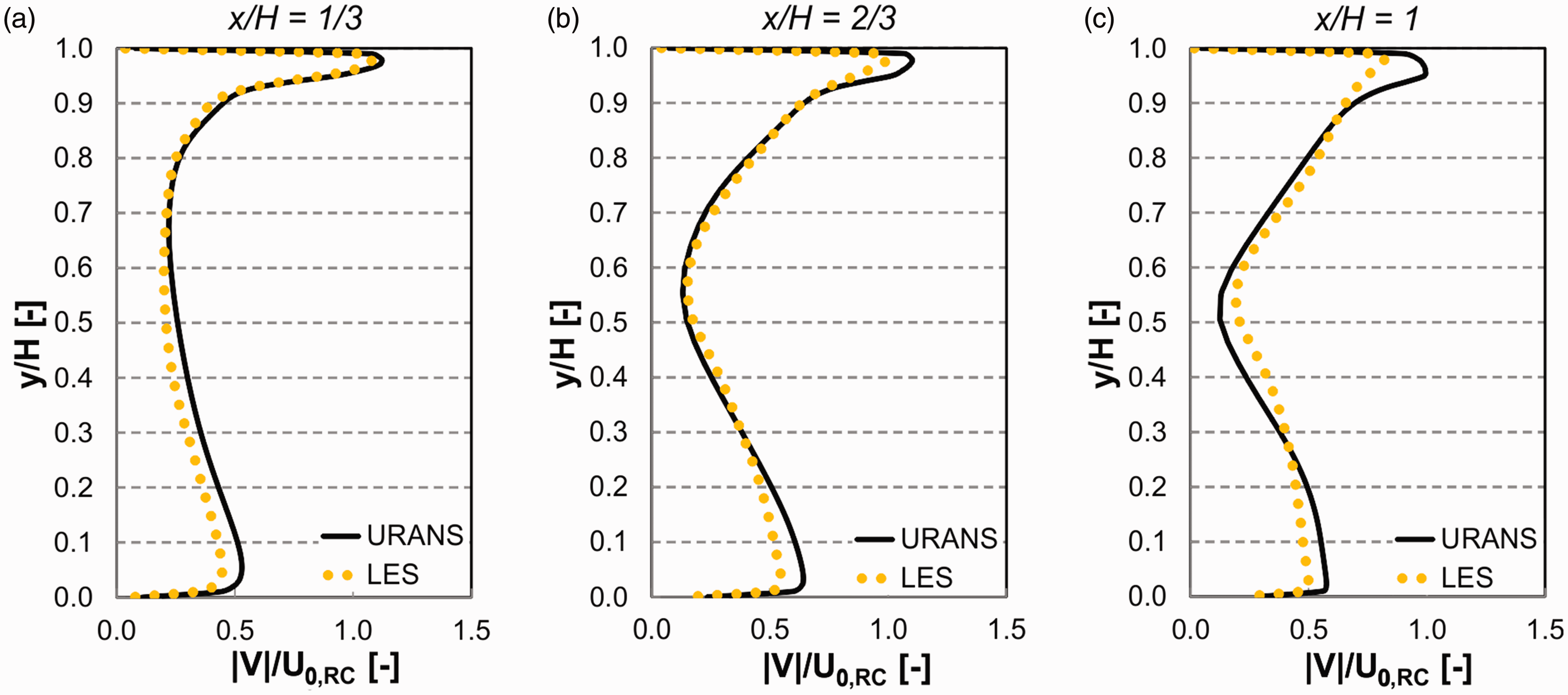
URANS vs. LES. |V|/U_{0 ,RC} along three vertical lines in the vertical centre plane (z/W = 0.5). (a) x/H = 1/3. (b) x/H = 2/3 and (c) x/H = 1.

Figure 19.

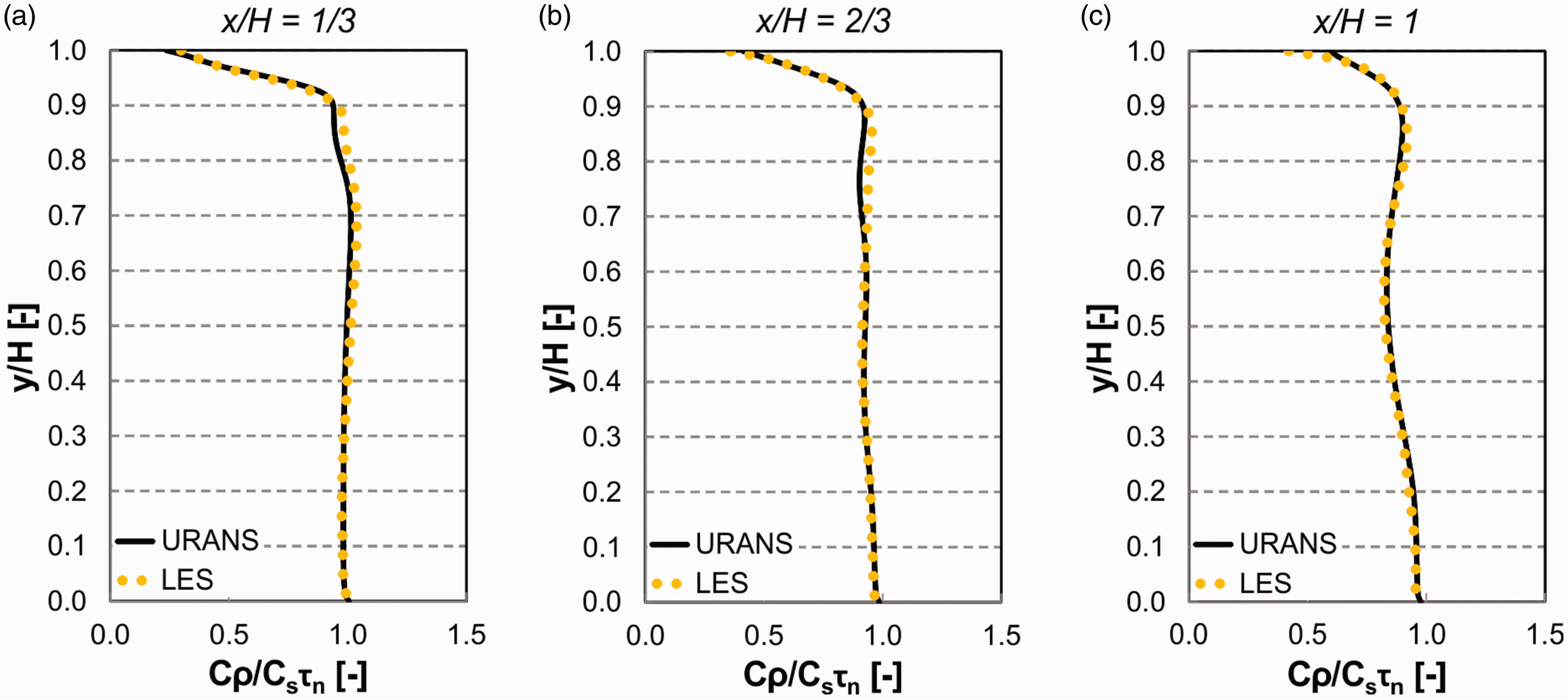
URANS vs. LES. Cρ/C_sτ_n along three vertical lines in the vertical centre plane (z/W = 0.5). (a) x/H = 1/3. (b) x/H = 2/3 and (c) x/H = 1.

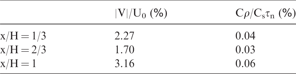
To quantify the agreement, the normalized mean square error (NMSE) was calculated for 300 values, i.e. 100 along each of the three vertical lines, using equation (6)

$$\mathrm{NMSE}=\frac{\overline{{\mathrm{(}\mathrm{L}\mathrm{E}{\mathrm{S}}_{\mathrm{i}}\text{-}\mathrm{URAN}{\mathrm{S}}_{\mathrm{i}}\mathrm{)}}^{\mathrm{2}}}}{\overline{\mathrm{L}\mathrm{E}{\mathrm{S}}_{\mathrm{i}}}\overline{\mathrm{URAN}{\mathrm{S}}_{\mathrm{i}}}}$$

(6)

where URANS_i and LES_i are the values obtained from URANS and LES, respectively, and the overbar indicates averaging over the 300 data points. Table 3 shows the values of NMSE indicating a very close agreement between URANS and LES. The maximum NMSE for |V|/U₀ is 3.2%, while the maximum NMSE for Cρ/C_sτ_n is only 0.06%. The results clearly indicate that the time-averaged results in URANS do not considerably differ from the results obtained with LES and that URANS is thus a suitable method to analyse time-periodic ventilation flows in a generic enclosure, with a reduction of computational time for URANS compared to LES.

Table 3.

NMSE for URANS vs. LES for time-averaged values of dimensionless velocity magnitude (|V|/U₀) and pollutant concentration (Cρ/C_sτ_n).

	|V|/U0 (%)	Cρ/Csτn (%)
x/H = 1/3	2.27	0.04
x/H = 2/3	1.70	0.03
x/H = 1	3.16	0.06

Limitations and future work

This study showed the potential of time-periodic supply velocities to enhance mixing in a generic enclosure subjected to mixing ventilation. The CFD simulations consisted of URANS simulations, and a comparison was made with LES. The study was subjected to a few limitations, which can incite future research efforts with focus on:

An experimental analysis of time-periodic ventilation flows in a generic enclosure. The experimental data obtained can also be used for CFD validation purposes.

The assessment of enhanced mixing for one-sided mixing ventilation flows and other cases in which mixing ventilation flow can be used to provide a healthy indoor environment.

The assessment of other periods and amplitudes to find an optimal combination of both with respect to mixing in an enclosure.

The analysis for intermittent (ON/OFF) or other types of time-periodic supply conditions.

Extension of the results for this specific generic geometry to more practical cases; i.e. realistic geometries, including buoyancy forces, other heat and momentum sources and sinks, etc., including a detailed analysis of energy consumption by the fans and the heating and cooling demand.

More detailed analyses of the convective and turbulent mass fluxes and other flow properties in an enclosure driven by time-periodic supply jets.

The effect of time-periodic mixing ventilation on thermal comfort and thermal sensation, for example using full-scale tests in climate chambers.

The use of computationally less demanding numerical methods to allow a faster exploration of the effects of time-periodic supply conditions.^46–48

Conclusions

This paper presented the first results in a broader research effort on the enhancement of mixing in mixing ventilation flows. URANS CFD simulations of mixing ventilation flow in a generic enclosure subjected to both constant supply velocities and time-periodic supply velocities were conducted for different cases. In all cases, two oppositely located supply openings in the upper part of the enclosure were present, while two oppositely located exhaust openings were present in the lower part. In addition, a comparison between the results from the URANS simulations and from LES simulations was made to verify the chosen turbulence modelling approach.

From this study, the following main conclusions were made:

The validation study showed the good performance of the RNG k-ε turbulence model in predicting mixing ventilation flows; differences in mean velocity were generally within 10–20%, while 80% of the predictions of TKE were within 30% from the measurement results.

The velocity and pollutant concentration fields were more uniform in the time-periodic supply case than in the constant supply case. High pollutant concentrations in the enclosure were strongly reduced due to the breakup of recirculation cells and the movement of stagnant regions.

The CRE was increased from 96% to 116% when time-periodic supply velocities are used.

The results obtained with three different periods T (T = 0.1τ_n, T = 0.2τ_n, T = 0.4τ_n), showed a negligible influence on the time-averaged velocities and pollutant concentrations, and on the CRE.

Compared to RC and RC_KE, time-periodic supply velocities could significantly improve mixing, reduce the high pollutant concentrations in the stagnant regions, and increase the CRE at equal (RE_KE) or lower (RC) fan energy use (when neglecting fan efficiency). The CRE in both reference cases is almost equal (within 1%), however, in RC_KE the volume-averaged concentration is 10% lower than in RC due to the higher supply velocity in RC_KE to obtain equal time-averaged kinetic energy levels of the supply flow as in the time-periodic case.

The LES results only showed marginal differences from the URANS results: NMSE for |V|/U_0,RC along three vertical lines is < 3.2%, while NMSE for Cρ/C_sτ_n along these three vertical lines is < 0.06%. This implies that for this study URANS can be considered sufficiently accurate, which reduces the computational demand compared to the use of LES.