Sage Journals: Discover world-class research

Abstract

This article analyses the movement of intergenerational mobility (IGM) in South Asia from birth cohorts comprising 1950–1980 using the World Bank’s data on IGM. The article compares the IGM movements across countries to account for the causal factors of the IGM. Exploratory data analysis and Bayesian regression have been used in this study for empirical analysis. We note that in the past three decades, the share of primary parental education in South Asia constitutes 79% of the total, while the children who achieved the highest level of education constitute only 10%. Children in Sri Lanka have been enrolled in school for the greatest number of years, but the absolute IGM in India is greater than Sri Lanka. Bhutan lags in average years of educational attainment, yet their relative mobility surpasses every country in South Asia. The likelihood that Pakistani children’s status shall be independent of their parental status is as low as 20%. Despite variation in parental education, absolute IGM in India is highest in South Asia. Variation in parental education reduces the degree of independence in the next generation. Relative measure of mobility is a better indicator of social mobility than the absolute measure.

JEL Codes: I21, I24, I28, J24, J62, N35

Keywords

Intergenerational mobility inequality education economic growth South Asia

Introduction

The developing economies of South Asia have experienced continuous economic growth in the past three decades. A rise in the gross domestic product (GDP) from 2.5% in the 1990s to as close as 7.5% in 2021 (World Bank, 2021a), South Asian nations have led the growth chapter in the world against the global average growth rate of 3%. Technological advancement, developmental projects and trade openness have brought about investment in these economies, leading to a sharp rise in growth rates (Bhavan et al., 2011; Mughal et al., 2022; Rahman et al., 2019). Most of the growth story among South Asian nations is associated with India where the booming tech industry and urbanization have contributed to rapid growth. Similarly, Bangladesh has played a key role in contributing to the growth by enhancing its manufacturing sector. The textile industry in Bangladesh accounted for nearly 86% of its exports in July–December 2022 (Export Promotion Bureau, 2023). However, one needs to have an eye for detail in the uniform distribution of economic progress as far as South Asia is concerned. One such area of concern is the area of social mobility. Social mobility may be defined as the extent of the rise in status of one generation with respect to its previous generation.

There have often been debates and research papers on economic inequality since its realization (Alfani et al., 2022; Casara et al., 2022; Jangvithaya, 2021). Yet, the degree of transmission of economic inequality from one generation (intergenerational mobility [IGM]) to the other has recently become the topic of discussion among academia and researchers (Black & Devereux, 2011). Increment in mobility across generations create equality of opportunity in a country, thereby fostering development and advancement at a rapid pace. Nordic countries¹ are the best examples of such progress in the twenty-first century (Corak, 2013). Studies show that there are a multitude of factors influencing social mobility and that these factors may vary across countries and continents with roots in historical migration or colonial past or government policies (Alesina et al., 2021; Asher et al., 2018; Neidhöfer et al., 2018).

Although IGM has been studied in detail by researchers across the globe, most of the study focuses on European nations. Few draw attention towards Latin America (Neidhöfer et al., 2018) and some towards African countries (Alesina et al., 2021). South Asian nations have largely been unexplored primarily due to a lack of data availability until recently. Also, the measure of IGM in previous studies, particularly European, has been the ‘permanent incomes’ of families across generations. Such datasets for Asia are largely unavailable. While income would undoubtedly serve as a good measure of IGM, it is equally difficult and practically impossible to gather income data across generations for developing South Asian economies. Thus, in line with the practical considerations and current conventions, we have used education as a measure of IGM.

Educational achievement in South Asia is one of the mixed successes. The enrolment ratios for secondary and tertiary education are low and the regional literacy rate is 62.4% (Asian Development Bank, 2016). This region has a high percentage of young population, an estimated 620 million children and adolescents live in eight countries of South Asia. The countries are Afghanistan, Bangladesh, Bhutan, India, Maldives, Pakistan, Sri Lanka and Nepal. Despite sociocultural diversities, these countries have come forward to promote educational well-being of their citizens. As such, countries like India and Nepal have granted education as a constitutional right. Similarly, South Asian nations have entered into international treaties such as the Convention on the Rights of Child (CRC) that recognizes the universal norm of the right to education. Yet, the committee on CRC noted that there is a gap between legal commitment and reality as far as the implementational policies are concerned (UNICEF, 2020). Gender gaps have gradually closed in primary schooling, while in some countries, it has begun to close with gender parity in primary education enrolment standing close to one for countries like Sri Lanka and Maldives. Recently, the World Bank’s Global Database on Intergenerational Mobility (GDIM) has published IGM as a measure of education (World Bank, 2020). Not only does education serve as a comprehensive measure of IGM, but it also is an indicator of the future incomes and productive capacity of a nation.

We have chosen to take up the task of studying IGM in South Asia for the following reasons. First, South Asian nations have experienced tremendous growth in the last three decades, with a fair Gini index ranging between 0.3 and 0.4. Yet, less than 9% of individuals whose parents’ education level was in the bottom half of the population reached levels of education of the highest educated 25% (World Bank, 2021b). Studying IGM through education has several advantages. First, it is considered an important criterion of well-being and has a close association with income mobility (Torche, 2021). Second, the data on education is more accurate than income data because respondents in the survey can better report their levels of education than their income in the past. Moreover, the study of IGM reveals the amount of opportunity prevailing in society. It has been observed that inequality of opportunity is more detrimental to growth and societal cohesion than inequality of outcomes (Bussolo et al., 2019; Ferreira et al., 2018; Marrero & Rodríguez, 2013; Narayan et al., 2018). It is also linked to the rate of economic growth and the associated change in occupational structure. Second, this study shall also bring to light whether the fruits of economic growth in the last two decades have percolated down to the bottom half of the population. In other words, we would like to see the status of educational mobility in the past 30 years for the bottom half of the population through the metrics developed by the World Bank. According to Asher et al. (2018), IGM in India has improved for certain sections of society and simultaneously fallen for other groups, reflecting unevenness in mobility.

Third, to the best of our knowledge, there has not been a significant study yet that primarily focuses on South Asian nations. We chose to fill this gap by analysing IGM across the nations. Our contribution to the existing literature uniquely includes exploratory data analysis of absolute and relative measures of IGM in South Asia. We have tried to analyse the trends in IGM across several birth cohorts of individuals to account for the plausible causes of social mobility. In doing so, we have plotted the absolute and relative measures of IGM of the South Asian countries² and examined the trends given the existing literature on causal factors of IGM. Further, we have framed our hypothesis based on our exploration and theory and ran regressions to account for the major contributors of social mobility in South Asia.

The ‘Review of Literature’ section of the article constitutes the literature review. The ‘Theoretical Background and Research Hypothesis’ section is about the theoretical background of IGM and hypothesis development, while the ‘Data and Definitions’ section discusses the variables and data sources. The ‘Methodology and Model Framework’ section is devoted to methodology and framework, while the ‘Empirical Analysis and Discussion’ section contains empirical analysis. In the ‘Conclusions and Policy Suggestions’ section, we conclude the article with policy suggestions.

Review of Literature

Major studies on IGM focus on European nations, the United States (US) and Canada (Van der Weide et al., 2021). While some have preferred to study its association with inequality and growth, others have used measures independent of the duo. Corak (2013) used the ‘Great Gatsby Curve’ to explain the change in IGM along with income inequality in the US, United Kingdom (UK), and Italy along with Nordic countries. Income disparities in a country tend to reinforce economic advantages and disadvantages between parents and children. The Great Gatsby Curve is an illustration of the concentration of wealth of one generation and the ability of the next generation to move up the ladder of income compared to their parents. Corak (2013) uses ‘permanent incomes’ for individuals from a particular family across two generations to estimate the intergenerational earning elasticity that measures the ‘stickiness of earnings’ across generations within the family.

The models to study the causal factors influencing IGM go back to Becker and Tomes (1986). They build their model upon the utility maximization principle of parents who are concerned about the welfare of their children. Their conclusion regarding IGM is that almost all economic advantages or disadvantages held in a generation are erased after the passage of three generations. Solon (2004) built upon their research in a way appropriate for making comparisons across countries and over time. He underscores the importance of education by taking the return to school as an indicator of the degree of inequality in the labour market and shows that societies with labour markets characterized by more cross-sectional inequality—reflecting in part a higher return to education—will be less generationally mobile. According to Solon (2004), two countries may spend the same fraction of their GDP on education, but their returns are likely to differ based on the direction of investment made. Expenditures directed towards high-quality early childhood primary and secondary education—accessible to all—is likely to improve IGM than expenditures directed towards tertiary education accessible to few. Looking at the metrics of educational expenditures, we see that countries having similar budget for education seems to resonate with Solon’s argument. For example, the average educational expenditure of Afghanistan and Sri Lanka in the period 1970–2019 has been around 2.53% of the GDP. Yet, both countries differ in their IGM status. Sri Lanka’s absolute IGM (0.57) is greater than that of Afghanistan (0.41) for the birth cohort 1980. Another example is that of Russia and Rwanda. Both countries have spent approximately 3.7% of the GDP on education during the period 1970–2019 but differ in IGM significantly. Russia is way ahead in IGM than Rwanda. Comparing the IGM of UK and US, it is found that UK’s absolute IGM is 0.68, while that of US’s is 0.47 for the birth cohort 1980 and both countries have spent, on an average, around 5% of their GDP on education during the period 1970–2019 (Educational Expenditure Statistics, World Bank, 2022).

Looking at IGM from other perspectives, Mountford-Zimdars and Sabbagh (2013) say that among the hindrances to social equality of opportunity (IGM), in the context of higher education, is the persistence of irreducible differences between families in income, social and cultural resources. Though governments can partly facilitate the economic differences, they cannot eliminate the contribution of family through cultural capital and social networks. This also suggests that segregation in societies can be an obstacle to the rise in social mobility and that lacking social and cultural capital influences IGM negatively. Socially advantaged families are better at using educational structures to advance their position, for example gaining access to selective universities (Marginson, 2016; Shavit, 2007).

Recent studies on IGM include Gu et al. (2022), who highlighted intergenerational educational mobility considering educational expansion in China since 1999. According to their research, the nine-year compulsory education policy launched by the Chinese Government in 1986 has had a lasting effect on the two generations’ education. They examined the role of parental input in accessing higher education in the context of the 10-fold expansion of China’s higher education sector since 1999.

IGM in Africa was examined by Alesina et al. (2021) to answer questions on educational opportunity, gender disparities and the rural–urban gap in education. Using one of the absolute upward mobility measures, defined as the likelihood of children born to parents without primary education, the article draws attention to the heterogeneous nature of IGM in African countries. While South Africa and Botswana’s educational attainment exceeds 70%, the corresponding statistic in Sudan, European Mozambique and Malawi hovers below 20%. Regional variations were also taken into account such that in countries like Kenya, whose average upward mobility is 50%, the likelihood that children born to illiterate parents would complete primary education varied from 5% (Turkana a region) to 85% (Westlands in Narobai). Similar studies have been carried out for the US (see Black & Devereux, 2011; Card et al., 2018; Solon, 1999).

Public interventions are of paramount importance when it comes to the improvement in IGM as countries become richer. Unequal access to good-quality schools can hamper IGM. Arenas and Hindriks (2021) suggest that IGM can be increased through school equalization interventions and desegregation policies. The absence of public interventions will decrease mobility, particularly in lower income countries. Children born to highly educated parents are twice fortunate since not only do they benefit from the exposure of their parents’ higher human capital but also from the investment (monetary) they make on their children (Becker et al., 2018; Duncan & Murnane, 2011). Effective public interventions stipulate that governments must invest in human capital at an early stage of childhood (Herrington, 2015; Lee & Seshadri, 2019; Restuccia & Urrutia, 2004). This would level the ‘playing field’ and serve to increase the ‘equality of opportunity’ among the various sections of income groups.

Cross-country analysis of IGM conducted by Neidhöfer et al. (2018) reveals new realities in Latin American countries. The study provides datasets for 18 countries and measures IGM correlation with macroeconomic variables and institutional characteristics. They find that IGM, on average, is on a rising trend in Latin America and that cross-country IGM is significantly related to economic performance and more progressive public spending in the educational system. It is the decline in income inequality since 2000 that has contributed to the rising IGM in Latin America. The literature review process of the article found that there is a less significant study on South Asian countries. The present analysis fills that context.

Theoretical Background and Research Hypothesis

IGM, theoretically, is closely linked to the transmission of the economic inequality of one generation to the other as ‘inheritability of earning ability’ (Neidhöfer et al., 2018) and the parental investment in the human capital of their children. Thus, parents maximize their utility through their own consumption and investment in their children. Moreover, it has been argued that a major substitute to private parental investment is the intervention of the government through public investment in the human capital of children. Most of the studies on IGM reveal that public intervention has a key role to play in influencing IGM (Alesina et al., 2021; Gu et al., 2022). We seek to investigate the impact of parental education on the educational attainment of children. Specifically, we have chosen parental education that belongs to the lowest categories of education (ISECED0 and ISECED1) to see its impact on the highest level of educational attainment. ISECED stands for International Standard Classification of Education (ISCED), a group of categories constructed by the United Nations Educational, Scientific and Cultural Organization, which classifies individuals based on their level of educational attainment.

Hypothesis of the Study

H₁: Low parental education negatively impacts high educational attainment.

The collective share of education of parents who have completed at most primary years of education negatively impacts the share of children to complete the highest level of education in a country over the period of birth cohorts. This means that a country where parental education is at the lower level may hinder the highest level of education for their children. Precisely, if the share of parental education at the lower level is huge, the likelihood that the share of the highest educational attainment for children will be low is quite high. Research shows that children born to highly educated parents are twice as fortunate since not only do they benefit from the exposure of their parents’ higher human capital, but also from the investment (monetary) they make on their children (Becker et al., 2018; Duncan & Murnane, 2011). In the back of the above discussion, the present hypothesis seeks to examine the impact of low parental education on high educational attainment in South Asia.

H₂: Variation in parental education negatively impacts intergenerational mobility.

Parental years of education in a country for each respondent vary significantly from the mean years of parental education. It is said to have high variability. Thus, a country with high variation in parental education should have a lower IGM. However, this variation can have a bidirectional effect. In the Indian context, there also seems to prevail high variation in parental education, but this variability has actually led to higher IGM (absolute) in their children, suggesting optimism of Indian parents regarding their children’s future social mobility. Conversely, Bhutan’s absolute mobility has declined despite the rise in variation in parental education (see Figure 4). This leads to the formation of the present hypothesis that whether variation in parental mobility impacts the IGM negatively.

H₃: Income level positively impacts intergenerational mobility.

The rise of income of individuals impacts IGM. Since the increase in parental income is assumed to maximize their own consumption and the welfare of their children (Becker & Tomes, 1986), we seek to see the impact of real income per capita on intergeneration mobility. It is assumed that in every decade children attain more education than their parents. Yet, the absolute IGM and degree of upward mobility of individuals independent of their parental status (relative IGM) are questions to answer. This hypothesis examines the impact of real income on absolute and relative mobility.

Data and Definitions

To understand IGM in South Asia, we have gathered data primarily from the ‘Global Database on Intergenerational Mobility’, World Bank (World Bank, 2020). The dataset covers descriptive statistics of the South Asian countries and key measures of absolute and relative IGM. We define the major variables under study below and their source, label and range is mentioned in Table 1. Among the important measures of IGM are:

Table 1.

Variable Description.

Indicator Name	Label	Data Source	Data Range
Dependent Variable
Probability that child from bottom half ends up in Q3	BHQ3	Global database on Intergeneration Mobility, World Bank (September 2021)	0–1
Absolute mobility based on 5 ISCED categories (condition on parent not having tertiary education)	CAT	Global database on Intergeneration Mobility, World Bank (September 2021)	0–1
Share of children with ISCED (5–8)	C5	Global database on Intergeneration Mobility, World Bank (September 2021)	0–1
Independent Variable
Share of parents with primary education or less	PE	Global database on Intergeneration Mobility, World Bank (September 2021)	0–1
Mean of parents’ years of schooling	MeanP	Global database on Intergeneration Mobility, World Bank (September 2021)	Any whole number
Standard deviation of parent years of schooling	SDp	Global database on Intergeneration Mobility, World Bank (September 2021)	Any whole number
Share of inequality in years of schooling between PSUs	MLD_psu	Global database on Intergeneration Mobility, World Bank (September 2021)	0–1
Real GDP per capita (Average GDP per capita for respective cohorts)	GDP	World Development Indicators	Any whole number (2015 dollars)

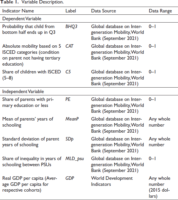
Dependent Variables

CAT—measures the absolute mobility of individuals, that is, the extent to which the living standard or income of a generation or educational attainment is higher than their parents. Here, CAT considers the educational attainment as per the World Bank definition. For example, suppose we have 100 respondents to the survey for a country, say X and the value of CAT = 0.41. This means that 41% of children received more education than their parents.

BHQ3—measures the relative mobility of individuals, that is, the extent to which social mobility of children is independent of parental status. To be precise, it is the probability that children from the bottom half of parents end up in the third quartile of the educated lot. In other words, what is the chance that children born to disadvantaged parents achieve education at the top level (more than 75% of the educated lot). To illustrate, if there are 100 educated people in a generation, what is the probability that a child born to a parent whose educational attainment is in the bottom half but their child manages to attain an educational level above 75% of the educated people in his generation.

C5—measures the share of children whose highest level of education translates to tertiary and above, which simply means children who have completed at least 15 years of education. C5 is one of the categories of educational attainment under ISCED. In the global database on IGM dataset, education level has been classified under several categories. A person with less than primary education is under ISCED 0 category, whereas a person with at-most primary education falls under ISCED 1 category and so on. C5 is defined as the share of children with ISCED (5–8) meaning children whose education is up to tertiary level.

Independent Variables

The independent variables under consideration are:

PE—This refers to the sum of less than primary (P1) and primary (P2) parental educational share for each country. Mathematically, PE = P1 + P2. Thus, we say that PE represents the share of parent respondents who have attained at-most primary education.

MeanP—This variable is the mean years of education for parents in each country.

SDp—This variable is the standard deviation (SD) of the educational distribution (in years) of parents in different countries. Technically, SD is the spread of educational years from its mean. To illustrate, if the SD of education for Indian parents during the period 1980–1989 is 3.77 which is approximately four years. This means that we can say that Indian parents have SD of around four years from their mean years of education during the 1980s.

GDP—It is the per capita GDP for each country.

MLD_psu—This variable is the share of inequality in years of schooling between public sector units. It is called ‘Educational Segregation.’ A higher inequality represents larger segregation and vice versa.

Methodology and Model Framework

We model the data with a Bayesian Framework. A Bayesian approach is applied to the dataset to account for the unobserved effect influencing the target variable. This approach allows us to resolve the issues pertaining to serial correlation, heteroscedasticity and multicollinearity. Our dataset is a panel type of data that combines time and cross-sections together. Each regressor belongs to a particular cross-section (here country) such that the influence it generates over the regressand is closely related to the nature of the cross-section. For example, the rate at which the ‘parental education’ changes in India is bound to be different from the ‘rate of change’ in Pakistan. Each parameter in the model is treated as a random variable, unlike the traditional approach to statistical inference. This makes it a more realistic model to incorporate in a panel setting. Thus, the unobserved factors are captured in the Bayesian approach making it a robust technique in economic analysis. Below we present the model framework for the statistical analysis.

C 5_{i t} = a_{i} + β_{1} P E_{i t} + β_{2} M e a n P_{i t} + β_{3} S D p_{i t} + β_{4} G D P_{i t} + β_{5} M L D_{_p s u_{i t}} + ϵ_{i t}

(1)

C A T_{i t} = a_{i} + β_{1} P E_{i t} + β_{2} M e a n P_{i t} + β_{3} S D p_{i t} + β_{4} G D P_{i t} + β_{5} M L D_p s u_{i t} + ϵ_{i t}

(2)

B H Q 3_{i t} = a_{i} + β_{1} P E_{i t} + β_{2} M e a n P_{i t} + β_{3} S D p_{i t} + β_{4} G D P_{i t} + β_{5} M L D_p s u_{i t} + ϵ_{i t}

(3)

The three equations above describe three different measures of IGM and its determinants. We seek to regress the highest educational attainment (C5) with parental education (PE), mean years of parents schooling (MeanP), SD of parental years of education (SDp), real income per capita (GDP) and the educational segregation (MLD_psu). CAT represents absolute IGM. It is defined as the extent to which children attain more education than their parents. Moreover, BHQ3 is the relative IGM. It is defined as the degree to which children’s status in society is independent of parental status. Parental education (PE) is the share of parental years of education in the ISCED (5–8) category. Educational segregation is the share of inequality in years of schooling between PSUs. In the dataset, we find that the MLD_PSUs for India from 1950 to 1980 birth cohorts decreased from 0.39 to 0.22. This indicates that inequality of years of schooling has gradually reduced over the course of 40 years. The subscripts, ‘i’ stand for the ith country and ‘t’ its corresponding time period. Time period t has been pooled across birth cohorts. We interpret a particular variable as, say, MeanP_Ind1980 as the average parental education years for the individual born between 1980 and 1989 in India. For example, in the dataset, we find that the mean years of schooling for Indian parents in the 1950s were 1.69 years. This means that in the period ranging 1950–1959, Indian parents attended roughly two years of schooling.

The general equation of the Bayesian model is as follows:

Y_{i j} = α_{i} + β_{i j} X_{i j} + ϵ_{i j}

(4)

where $Y_{i j}$ refers to the score of the outcome variable; $X_{i j}$ refers to the set of predictors; $α_{i}$ refers to the intercept of the dependent variable; $β_{i j}$ refers to the slope coefficients; $ϵ_{i j}$ refers to the random errors of prediction.

The coefficients in the model are not treated as fixed numbers. Instead, each parameter is a random variable with a probability distribution. The pdf of this random variable is called the priori. The model develops a priori for each parameter and executes it with the likelihood function of the outcome variable.

Empirical Analysis and Discussion

We begin our analysis with the descriptive statistics for the variables under study for the South Asian nations. Then, we proceed further with exploratory data analysis and try to understand the trends in educational attainments and IGM across the nations and look at each country’s performance. This follows the regression analysis of our dependent variables with the independent variable and its results.

Table 2 shows the descriptive statistics for the variables considered in the model. PE—it is the sum of P1 and P2, which means the share of parents who attended most primary education. Thus, 79% of parents have attained maximum up to primary education in South Asia, while only 1% of parents, on average, attended the topmost education in three decades. Against 1% of topmost education for parents, 10% of children attended topmost education. Apparently, it seems to be a rise in IGM. However, if we compare it with the primary education lot, we conclude that in 79% of parents who achieved primary education, only 10% of the children from them could afford topmost education.

Table 2.

Descriptive Statistics.

VARIABLES	MEAN	STD DEV.	MIN	MAX
P1	0.58	0.30	0.04	0.93
P2	0.21	0.09	0.06	0.41
PE	0.79	0.23	0.31	1.00
P3	0.14	0.15	0.00	0.44
P5	0.01	0.01	0.00	0.04
C5	0.10	0.08	0.02	0.25
MEANP	2.81	2.59	0.27	7.92
MEANC	5.54	2.67	1.95	9.94
BHQ3	0.22	0.02	0.19	0.26
CAT	0.40	0.16	0.13	0.61

Note: P1—share of parents with less than primary education; P2—share of parents with primary education; PE—sum of less-than primary (P1) and primary (P2) parental educational share for each country: PE = P1 + P2; P3—share of parents with lower secondary education; P5—share of parents with tertiary education; MEANp—mean of parents’ years of schooling; MEANc—mean of children’s years of schooling; BHQ3—probability that child from bottom half ends up in Q3; CAT—absolute mobility based on five ISCED categories (condition on parent not having tertiary education).

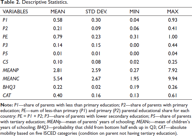
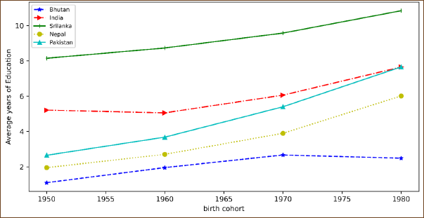
Figure 1 describes the mean educational distribution of children in South Asian countries. While Sri Lanka stands unique among other nations, Bhutan seems to have lagged behind. Individuals born in the 1980s attended more than nine years of education in Sri Lanka. The plot also reveals the resilience of Pakistan. With an average educational attainment of close to three years in the 1950s, it climbed up the ladder catching up with India in the 1980s to more than seven years. It is to be noted that the plot does not reflect IGM. It simply suggests the trends in education for South Asian countries and gives us a broader picture of mean educational distribution in the region. The poor performance of Bhutan can be explained simply by looking at the educational distribution of parents. Next, we present the absolute measure of IGM below.

Figure 1.

Cross-country Trends in Complete Attainment of Education of Children.

Comparing Figure 2 with Figure 1, we observe some startling facts about social mobility in South Asia. Though Sri Lanka seems to have taken the lead in mean years of education, leaving behind India and other countries, apparently reflecting impressive social mobility in the country, the IGM trend curves reveal new realities. IGM for India and Sri Lanka was almost the same in the year 1975–1977 despite the fact that children in India attended less years of education on average than in Sri Lanka. In fact, India’s IGM took over Sri Lanka in the early 1980s, that is, Indian children were 60% more educated than their parents, while Sri Lankan children were approximately 58% more educated than their parents. This reflects that Indian parents have been more optimistic about the future of their children and that they expect their children to be at a higher status than their own. Next, we discuss relative IGM in Figure 3.

Figure 2.

Intergenerational Mobility Across Nations.

Figure 3.

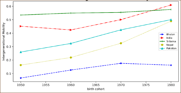
Cross-country Relative Intergenerational Mobility.

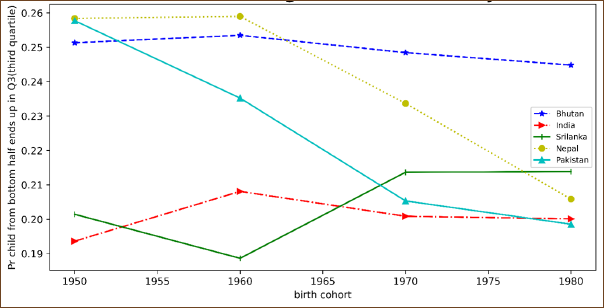
The plot above is the probability distribution of children born from bottom half parents, who may end up securing a status in the third quartile of educated children. Note that relative IGM is defined as the degree of social mobility of one generation independent of the position of his or her parents. In this context, Bhutan stands unique among all other South Asian Nations. Nepal, which stood along with Bhutan in the 1950s, has fallen down to 21%. Thus, the probability that individuals in Nepal, born to the bottom half parents in the 1980s, would climb up the ladder is 0.21. This reflects more dependence of the individual on parental status. Moreover, public intervention through school equalization seems to be low over the decades. The same is true for Pakistan. Relative IGM in India is also low. The Sri Lankan State has, however, managed to take over India as far as relative IGM is concerned. It jumped from 19% in the 1960s to 21% in the 1970s and managed to remain constant till the 1980s. Next, we present the movement of absolute mobility with respect to variation in parental education. We have taken into account four birth-decade cohorts (1950–1980) of mobility across the countries.

Figure 4 presents the scatter plot of absolute IGM and variance in parental education at different birth cohorts. If we look at the variation in the educational years of parents, we find that, generally, this variation has contributed to the rise in absolute upward mobility. This can be explained simply by thinking that parents who have attended less education send their children to school in the hope of a better future. India and Pakistan are perfect examples in the given curve. In the 1950s, while IGM for Pakistan was approximately 0.25, it rose to 0.50, with an increase in the variation of parental education in the 1980s. This suggests that despite the widening of the gap between parental educations, mobility as a whole has increased. In other words, children were better off than their parents. The same is true for India in the long run. However, we note one important point regarding India. In the 1950s, parents were not optimistic about educational attainment. Despite the increase in the variability of parental education, the absolute mobility dropped down from 0.45 to 0.40. However, the mobility curve climbed upward from the 1960s so much so that India’s absolute mobility is the highest among the South Asian nations reflecting optimism among parents for future generations. Next, we discuss the relative mobility curve with respect to the variability of parental education.

Figure 4.

Cross-country Relative Intergenerational Mobility.

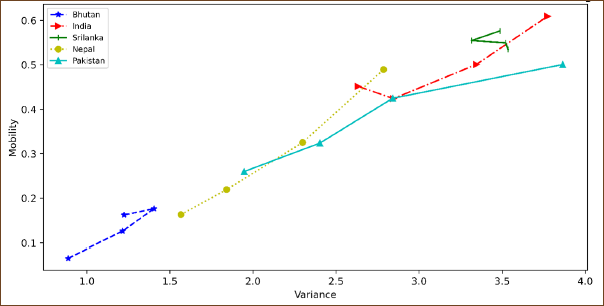
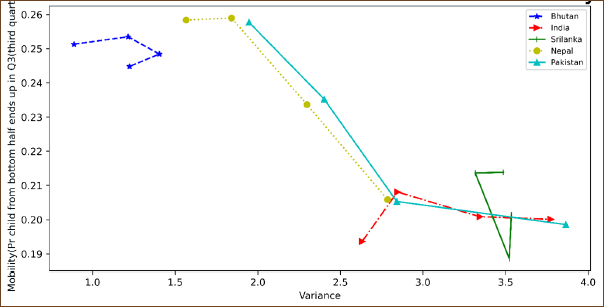
Figure 5 reveals the degree of independence of children status against parental status. Relative mobility is defined as the extent to which the social mobility of children is independent of parental status. We examine the trends in IGM across the nation with variations in the educational years of parents. While the IGM absolute (Figure 4) increased despite a widening gap in the educational years of parents, IGM relative (Figure 5) fell with the widening gap of educational years of parents. This reveals the interdependence of children on parents in South Asia. Moreover, this also suggests that if the gap between parental educational rises, children are less likely to be independent of their status in the long run. The case for Nepal shows that relative mobility has fallen continuously from the 1960s to the 1980s with the increase in variation of parental education. The same is true for India and Pakistan. However, the Sri Lankan state has managed to keep its relative mobility constant despite the increase in variation from the 1970s to the 1980s. The case for Bhutan in the 1950s and 1960s contrasts with the general notion. Relative mobility has increased with a rising variation.

Figure 5.

Cross-country Relative Intergenerational Mobility.

Bayesian Regression Analysis

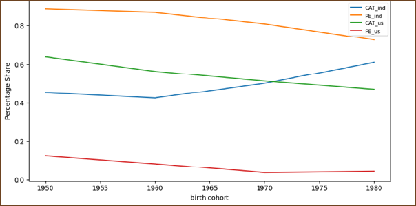
Having analysed IGM graphically, we use Bayesian regression on our dataset to account for the impact the explanatory variables under consideration make on educational attainments and IGM as per Equations (1)–(3). The share of primary parental education negatively related to absolute IGM (CAT). We notice that there is a rise in absolute IGM (CAT) with the decrease in share of primary parental educational years with the passage of time in South Asia. However, this rising absolute IGM and falling primary share is not true for advanced economies like the US. For example, Figure 6 presents the trends of absolute IGM and the primary share of parental education between the US and India. Clearly, we see that between 1950 and 1980 birth cohorts, absolute IGM has increased—reflecting a greater extent of education of children than their parents—in India. While in the US, IGM has fallen—reflecting a lower gap between parent–children’s educational levels. In an economy where educational levels are already high, IGM tends to be falling over the years.

Figure 6.

Note: CAT represents the absolute IGM while PE is the share of primary and less than primary parental education.

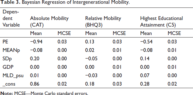
In contrast, relative mobility (BHQ3) is positively related to primary parental education (PE) (see Table 3). Note that BHQ3 is the probability that children, born to disadvantaged parents, end up in the third quartile of the educated lot in that generation. So, if there is a rise in the primary parental share, it is likely that relative mobility increases. If we look at the variation in parental education (SDp) and the measures of IGM, we note the following: (a) variation in parental education (SDp) is positively related to absolute mobility (CAT) and highest educational attainments (C5), while (b) variation in parental education (SDp) and relative mobility (BHQ3) are negatively related. Thus, we say that the higher the variation in parental educational years, lower the relative mobility—reflecting lower independence among the generation. This suggests that a lower level of educational qualifications of parents hinders top educational attainment in the next generations. Existing literature on IGM confirms this conclusion. Children born to socially advantaged families are twice fortunate as those born to socially disadvantaged parents (Becker et al., 2018; Duncan & Murnane, 2011). The GDP per capita coefficient is negligible to all the measures of IGMs and educational attainment. If we observe the relationship between educational segregation (MLD_psu) and the measure of IGMs, we note the following: (a) educational segregation is positively related to absolute IGM (CAT) and highest educational attainment (C5), while (b) it is negatively related to relative mobility (BHQ3). Thus, we say that rising inequality in educational years of schooling is likely to hinder independence and hence relative mobility. We will present the conclusion and policy suggestion of the article in the next section.

Table 3.

Bayesian Regression of Intergenerational Mobility.

Dependent Variable	Absolute Mobility (CAT)		Relative Mobility (BHQ3)		Highest Educational Attainment (C5)
	Mean	MCSE	Mean	MCSE	Mean	MCSE
PE	−0.94	0.03	0.13	0.03	−0.54	0.03
MEANp	−0.08	0.00	0.02	0.01	−0.08	0.01
SDp	0.20	0.00	−0.05	0.00	0.14	0.00
GDP	0.00	0.00	0.00	0.01	0.00	0.01
MLD_psu	0.01	0.00	−0.03	0.00	0.07	0.00
_cons	0.86	0.02	0.18	0.03	0.28	0.02

Note: MCSE—Monte Carlo standard errors.

Conclusions and Policy Suggestions

This article intends to track social progress in South Asia using the IGM of education as an indicator of progressivity. Greater independence in the status of one generation with respect to its previous generation is a good indicator of progress for a country. It reflects financial independence and greater mobility in society. Countries with greater mobility grow uniformly, thereby tackling issues of persistent unemployment in the long run. Thus, we propose the relative measure of mobility as a better indicator of social progress in a country. To improve the relative measure, government intervention to equalize educational attainments is of paramount importance. This has also been suggested by Arenas and Hindriks (2021). From our analysis, we see that greater variation in parental education shall hinder independence in the next generation. Thus, investment in quality education at the early level will strengthen skills and increase productive capacity in the future. We see this in the case for Pakistan or India or Nepal. Each country’s ability to produce independent future generations has gone down. For Pakistan, in the 1950s, the probability that a child born from bottom parents would climb up the ladder of the third quartile of the educated lot was 26%. In the 1980s, that ability fell to 20% despite an increase in absolute upward mobility from 26% in the 1950s to as close as 50% in the 1980s (see Figure 3). The same is true for Nepal and to a certain extent for India. What explains this simultaneous absolute rise and relative fall? We believe that two countries may spend the same fraction of their GDP on education but with different outcomes. Expenditure directed towards good-quality education at an early age—accessible to all—is bound to bear fruits uniformly rather than expenditure directed towards higher education—accessible to few. Looking at Figure 5, we observe that greater the variability of parental education—reflecting inaccessible early education to all—lowers the relative mobility—reflecting socially disadvantaged children. This is also confirmed by our regression analysis which shows a negative relation between variability in parental education and relative mobility. IGM is important to the policy makers since it helps in analysing the fairness and equality of opportunity in a society. A society having high mobility reflects greater economic efficiency and long-term economic growth, while those with low mobility reflect economic stagnation and misallocation of human capital. Thus, IGM becomes an important indicator for the policy makers in evaluating their policy decisions. This study will help policy makers to suggest policy decision based on the status of IGM in South Asia. However, this study has limitations due to the unavailability of parental income data that would provide better intuition and understanding of the nature of IGM in South Asia. Moreover, accounting for heterogeneity among nations—the size of the economy—and within nations, particularly communities and historical migration, would give us more insight into social mobility.

Footnotes

Declaration of Conflicting Interests

The authors declared no potential conflicts of interest with respect to the research, authorship and/or publication of this article.

Funding

We would like to acknowledge the funding under institute initiation grant by IISER Bhopal [grant number IISERB/R&D/2022-23/142] under which first author was hired as a Project Staff.

Notes

ORCID iD

Biswajit Patra

References

Alesina

, Hohmann

, Michalopoulos

, & Papaioannou

(2021). Intergenerational mobility in Africa. Econometrica , 89(1), 1–35. https://doi.org/10.3982/ecta17018

Asian Development Bank. (2016). Innovative strategies in higher education for accelerated human resource development in South Asia: Sri Lanka . Asian Development Bank Institute.

Arenas

, & Hindriks

(2021). Intergenerational mobility and unequal school opportunity. Economic Journal , 131(635), 1027–1050. https://doi.org/10.1093/ej/ueaa062

Alfani

, Gierok

, & Schaff

(2022). Economic inequality in preindustrial Germany, ca. 1300–1850. Journal of Economic History , 82(1), 87–125. https://doi.org/10.1017/S0022050721000607

Asher

, Novosad

, & Rafkin

(2018). Intergenerational mobility in India: Estimates from new methods and administrative data . World Bank working paper.

Bhavan

, Xu

, & Zhong

(2011). Determinants and growth effect of FDI in South Asian economies: Evidence from a panel data analysis. International Business Research , 4(1), 43–50.

Black

S. E.

, & Devereux

P. J.

(2011). Recent developments in intergenerational mobility. In Handbook of labor economics (Vol. 4, pp. 1487–1541). Elsevier. https://doi.org/10.1016/S0169-7218(11)02414-2

Becker

G. S.

, & Tomes

(1986). Human capital and the rise and fall of families. Journal of Labor Economics , 4(3 Pt. 2), S1–S39. https://doi.org/10.1086/298118

Becker

G. S.

, Kominers

S. D.

, Murphy

K. M.

, & Spenkuch

J. L.

(2018). A theory of intergenerational mobility. Journal of Political Economy , 126(Suppl. 1), S7–S25. https://doi.org/10.1086/698759

10.

Bussolo

, Checchi

, & Peragine

(2019). Long-term evolution of inequality of opportunity (Policy Research Working Paper Series 8700). The World Bank .

11.

Card

, Domnisoru

, & Taylor

(2018). The intergenerational transmission of human capital: Evidence from the golden age of upward mobility (No. w25000). National Bureau of Economic Research. https://doi.org/10.3386/w25000

12.

Corak

(2013). Income inequality, equality of opportunity, and intergenerational mobility. Journal of Economic Perspectives , 27(3), 79–102. https://doi.org/10.1257/jep.27.3.79

13.

Casara

B. G. S.

, Suitner

, & Jetten

(2022). The impact of economic inequality on conspiracy beliefs. Journal of Experimental Social Psychology , 98, 104245. https://doi.org/10.1016/j.jesp.2021.104245

14.

Duncan

G. J.

, & Murnane

R. J. (Eds.)

. (2011). Whither opportunity? Rising inequality, schools, and children’s life chances . Russell Sage Foundation.

15.

Export Promotion Bureau. (2023, January 5). Fibre2fashion.Com/.

16.

Ferreira

F. H. G.

, Lakner

, Lugo

M. A.

, & Özler

(2018). Inequality of opportunity and economic growth: How much can cross-country regressions really tell us? Review of Income and Wealth , 64(4), 800–827. https://doi.org/10.1111/roiw.12311

17.

, Hua

, McKenzie

, & Zheng

(2022). Like father, like son? Parental input, access to higher education, and social mobility in China. China Economic Review , 72, 101761. https://doi.org/10.1016/j.chieco.2022.101761

18.

Herrington

C. M.

(2015). Public education financing, earnings inequality, and intergenerational mobility. Review of Economic Dynamics , 18(4), 822–842. https://doi.org/10.1016/j.red.2015.07.006

19.

Jangvithaya

(2021). Will I be rich if I come from an impoverished family? MPFD policy brief , 122.

20.

Lee

S. Y. T.

, & Seshadri

(2019). On the intergenerational transmission of economic status. Journal of Political Economy , 127(2), 855–921. https://doi.org/10.1086/700765

21.

Mughal

, Arif

, Jain

, Chupradit

, Shabbir

M. S.

, Ramos-Meza

C. S.

, & Zhanbayev

(2022). The role of technological innovation in environmental pollution, energy consumption and sustainable economic growth: Evidence from South Asian economies. Energy Strategy Reviews , 39, 100745. https://doi.org/10.1016/j.esr.2021.100745

22.

Marginson

(2016). The worldwide trend to high participation higher education: Dynamics of social stratification in inclusive systems. Higher Education , 72(4), 413–434. https://doi.org/10.1007/s10734-016-0016-x

23.

Marrero

G. A.

, & Rodríguez

J. G.

(2013). Inequality of opportunity and growth. Journal of Development Economics , 104, 107–122. https://doi.org/10.1016/j.jdeveco.2013.05.004

24.

Mountford-Zimdars

, & Sabbagh

(2013). Fair access to higher education: A comparative perspective. Comparative Education Review , 57(3), 359–368. https://doi.org/10.1086/671194

25.

Neidhöfer

, Serrano

, & Gasparini

(2018). Educational inequality and intergenerational mobility in Latin America: A new database. Journal of Development Economics , 134, 329–349. https://doi.org/10.1016/j.jdeveco.2018.05.016

26.

Narayan

, Van der Weide

, Cojocaru

, Lakner

, Redaelli

, Mahler

D. G.

, & Thewissen

(2018). Fair progress? Economic mobility across generations around the world . World Bank Publications.

27.

Rahman

M. M.

, Rana

R. H.

, & Barua

(2019). The drivers of economic growth in South Asia: Evidence from a dynamic system GMM approach. Journal of Economic Studies , 46(3), 564–577. https://doi.org/10.1108/JES-01-2018-0013

28.

Restuccia

, & Urrutia

(2004). Intergenerational persistence of earnings: The role of early and college education. American Economic Review , 94(5), 1354–1378. https://doi.org/10.1257/0002828043052213

29.

Solon

(2004). A model of intergenerational mobility variation over time and place. Generational Income Mobility in North America and Europe , 2, 38–47.

30.

Shavit

(Ed.). (2007). Stratification in higher education: A comparative study . Stanford University Press.

31.

Solon

(1999). Intergenerational mobility in the labor market. In Handbook of labor economics (vol. 3, pp. 1761–1800). Elsevier. https://doi.org/10.1016/S1573-4463(99)03010-2

32.

Torche

(2021). Intergenerational mobility in Latin America in comparative perspective (UNDP LAC Working Paper No. 02) . Background Paper for the UNDP LAC 2021 Regional Human Development Report.

33.

Van der Weide

, Lakner

, Mahler

D.G.

, Narayan

, & Ramasubbaiah

(2021). Intergenerational mobility around the world . http://dx.doi.org/10.2139/ssrn.3981372

34.

United Nations Children’s Fund (UNICEF). (2020). For every child, Reimagine. UNICEF Annual Report 2019.

35.

World Bank. (2020). Global database on intergenerational mobility (GDIM) . World Bank.

36.

World Bank. (2021a). World Development Indicators.

37.

World Bank. (2021b). World development report 2021: Data for better lives .

Intergenerational Mobility in South Asia

Abstract

Keywords

Introduction

Review of Literature

Theoretical Background and Research Hypothesis

Hypothesis of the Study

Data and Definitions

Variable Description.

Dependent Variables

Independent Variables

Methodology and Model Framework

Empirical Analysis and Discussion

Descriptive Statistics.

Cross-country Trends in Complete Attainment of Education of Children.

Intergenerational Mobility Across Nations.

Cross-country Relative Intergenerational Mobility.

Cross-country Relative Intergenerational Mobility.

Cross-country Relative Intergenerational Mobility.

Bayesian Regression Analysis

Bayesian Regression of Intergenerational Mobility.

Conclusions and Policy Suggestions

Footnotes

Declaration of Conflicting Interests

Funding

Notes

ORCID iD

References