
Abstract
The reassessment of engineering structures, such as bridges, now increasingly involve the integration of models with real-world data. This integration aims to achieve accurate ‘as-is’ analysis within a digital twin framework. Bayesian model updating combines prior knowledge and data with models to enhance the modelling accuracy while consistently handling uncertainties. When updating large engineering models, numerical methods for Bayesian analysis present significant computational challenges due to the need for a substantial number of likelihood evaluations. The novelty of this contribution is to parallelize adaptive Bayesian Updating with Structural reliability methods combined with subset simulation (aBUS) to improve its computational efficiency. To demonstrate the efficiency and practical applicability of the proposed approach, we present a case study on the Maintalbrücke Gemünden, a large railway bridge. We leverage modal property data to update a linear-elastic dynamic structural model of the bridge. The parallelized aBUS approach significantly reduces computational time, making Bayesian updating of large engineering models feasible within reasonable timeframes. The improved efficiency allows for a wider implementation of Bayesian model updating in structural health monitoring and maintenance decision support systems.
Keywords
Introduction
The design of engineering structures such as road and railway bridges is based on models. When re-assessing structures, models are still considered, but inspections and in-service data gathered using non-destructive testing (NDT), diagnostic load tests, or structural health monitoring (SHM) are also considered. Updating the structural models with these data provides ‘as-is’ structural analysis models that more closely represent the actual performance of an engineering structure. When performed continuously, it can be part of a ‘digital twin’ framework (Ye et al., 2022) that enables diagnostic, prognostic, and decision support tasks.
When translating research into practice, it is crucial to consider the efficiency of the updating process and the quality of the updated models (Ye et al., 2022). Bayesian methods are becoming increasingly popular (Ye et al., 2022) which is attributed to their robust handling of unavoidable uncertainties in measurement and modelling processes (Huang et al., 2019), along with their ability to incorporate and update prior knowledge with observed data for nuanced interpretations (Pai and Smith, 2022). In this contribution, we also leverage Bayesian methods for model updating. Bayesian model updating quantifies parameter uncertainty as relative plausibilities of different parameter values (Beck, 2010; Huang et al., 2019). Selecting the most suitable model class that best explains the measured data without overfitting (Beck, 2010; Beck and Yuen, 2004; Kontoroupi and Smyth, 2017) is crucial for ensuring the quality of the model updating process (Simon et al., 2024). Additionally, evaluating the relative plausibilities of competing model classes can further improve the quality of the model predictions (Beck, 2010; Beck and Yuen, 2004; Papadimitriou et al., 2001).
The requirements for Bayesian model updating methods for large engineering structures are as follows: First, they must be computationally efficient to handle large models and provide solutions within reasonable time frames. A relatively recent example of updating an engineering model of a large suspension bridge (Jang and Smyth, 2017) took 3 months to compute. Second, there should be the possibility of exploring high-dimensional parameter spaces because models of large structures may have many relevant parameters. Third, the model class selection process requires knowledge of the model evidence, also known as marginal likelihood (Beck, 2010; Huang et al., 2019).
The state-of-the-art methods for obtaining samples from the updated distribution of the model parameters are Markov Chain Monte Carlo (MCMC) methods (Lye et al., 2021). Three classes of MCMC methods provide estimates of the model evidence: (a) Transitional Markov Chain Monte Carlo (TMCMC) (Ching and Chen, 2007), (b) nested sampling (Koune et al., 2023; Skilling, 2004; Titscher et al., 2023; Xu et al., 2022), and (c) Bayesian updating with structural reliability methods (BUS) (Straub and Papaioannou, 2014), and its extension adaptive Bayesian updating with structural reliability methods using subset simulation (aBUS) (Betz et al., 2018b). The evaluation of the relative performance and accuracy of these methods is the subject of ongoing research (Smith et al., 2023). TMCMC can be parallelized (Goller et al., 2011), which greatly improves its efficiency. However, if the number of uncertain parameters is high, the potential for considerable bias arises, and the efficiency decreases (Betz et al., 2016). BUS with subset simulation promises to be applicable to high-dimensional problems. However, methods that fulfil all three requirements are missing.
We conclude that a method for Bayesian updating is needed which is efficient, works in high-dimensional parameter spaces, and provides an estimate of the evidence of a model class. A solution to closing this gap is to improve one of the three existing methods that provide an estimate of the model evidence. This could be done by addressing the performance issues of nested sampling or TMCMC when applied to problems with highly-dimensional parameter spaces. However, in our contribution we focus on improving the efficiency of aBUS through parallelization.
First, we introduce Bayesian model updating and aBUS. Then we show, how aBUS can be robustly parallelized. This is our primary contribution. Subsequently, we apply the parallelized version of aBUS to update a large finite element model of a railway bridge and evaluate the achieved speedup compared to the sequential version of aBUS. We complete the paper with a discussion and concluding remarks.
Bayesian model updating
Bayesian updating of (probabilistic) engineering models – like Bayesian inference of probabilistic models in general – can be performed on two levels: First, the probability distribution of the model parameters is updated with observed data, as briefly discussed in the following. Subsequently, the relative plausibilities of proposed candidate models are compared.
Parameter inference
To update the prior distribution p(
As a first step, a data prediction model is defined which relates the i-th observation

Next, a probabilistic model of the prediction error
Generically describing the covariance matrix
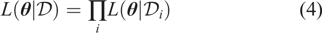
In order to learn the probabilistic distribution of the model parameters θ based on the observed data it is necessary to formulate a likelihood function. This function probabilistically describes the likelihood of observing the data given a certain realization of the model parameters θ. This formulation is based on the probability model of the prediction error and the data prediction model. We formulate a likelihood function
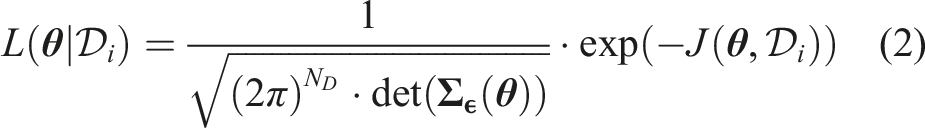

The prediction errors
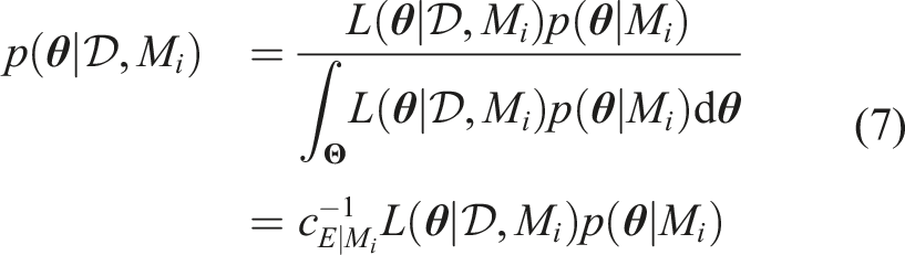
Applying Bayes’ rule yields the posterior probability density
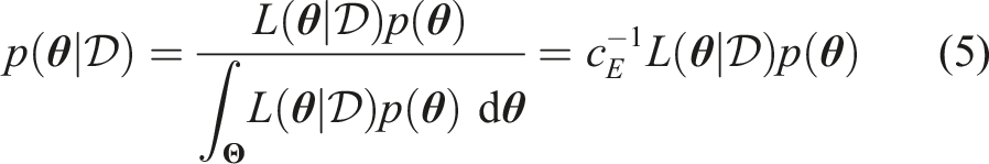
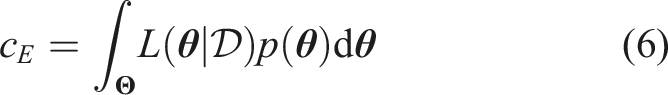
The normalizing constant c
E
is also referred to as model evidence:
Prior knowledge of the uncertain parameters
Model class selection
There are many ways of modelling a physical system. Furthermore, there are several ways of modelling the prediction error (Koune et al., 2023; Simoen et al., 2013). Consequently, we need a way of deciding, which way of modelling is more appropriate given the data.
To this end, we formally define a stochastic model class M i , as introduced in (Beck, 2010) which consists of: (1) a parametrized deterministic engineering model of the physical system, (2) a parametrized probabilistic model of the discrepancy between the model output and the observations, and (3) a joint prior probability density of the uncertain parameters of the deterministic engineering model and the probabilistic models, reflecting prior knowledge.
All the relations derived in the previous section depend on the modelling choices and assumptions encoded in a given model class M
i
, and thus equation (5) can be written as follows to reflect this dependence:
When the likelihood function is a proper probability distribution, that is,

When Bayesian model updating is performed within each model class M
i
of a set
With these conditions met, Bayes’ rule can be applied anew, yielding the posterior probability
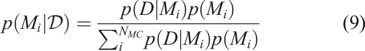
We now can select the model class among all postulated model classes that most appropriately explains the data. This procedure is also referred to as model class selection (Beck, 2010; Beck and Yuen, 2004). In physics-based structural health monitoring, this method can be leveraged both for selecting the most appropriate model for example (Simon et al., 2024) and for damage identification for example (Ntotsios et al., 2009; Simon et al., 2024).
Adaptive BUS combined with subset simulation
The challenge for Bayesian updating of engineering models is that there is rarely a closed-form solution for equation (5) available. Additionally, when the likelihood function contains a deterministic engineering model, it is not continuous but can only be evaluated at discrete values. To overcome this, Markov chain Monte Carlo (MCMC) sampling methods – such as the Metropolis-Hastings algorithm (Hastings, 1970; Metropolis et al., 1953) or modern derivatives (Betancourt, 2017) – are commonly employed to draw samples from the posterior distribution
The goal is to obtain samples representative of the posterior distribution, while at the same time minimizing the number of likelihood evaluations. An overview of various categories of currently available methods is given in (Lye et al., 2021).
For Bayesian updating of engineering models, there are two specific requirements: (1) Large engineering models typically have many uncertain parameters, which influence the structure’s behaviour and are thus of interest in the model updating. The applied method has to be able to cope with such high-dimensional problems. (2) Several modelling choices can be made, regarding the applied physical/mechanical theories, and the level of detail of the engineering model. To enable a comparison of competing model classes representing different modelling choices with model class selection, the model evidence has to be computed.
To meet these requirements, the adaptive variant of Bayesian Updating with Structural reliability methods combined with subset simulation (aBUS) (Betz et al., 2018b; Straub and Papaioannou, 2014) is employed in this contribution.
In the following, we describe the workings of aBUS in three steps: (1) the main idea of BUS is discussed, then (2) aBUS with subset sampling is presented, and subsequently (3) the adaptive Conditional Sampling algorithm as an MCMC sampler in aBUS is described.
The main idea of BUS
Bayesian Updating with Structural reliability methods (BUS) reframes Bayesian model updating as a structural reliability problem. BUS expands the parameter space
Straub and Papaioannou (Straub and Papaioannou, 2014) demonstrate that samples from the prior distribution p(
In the augmented parameter space

BUS typically involves applying sampling-based reliability methods to generate samples in the failure domain and compute c E . Implementing BUS with simple Monte Carlo Simulation is equivalent to rejection sampling. Subset simulation (Au and Beck, 2001) is preferred as it is efficient in high-dimensional problems and also directly produces samples within the failure domain.
aBUS algorithm
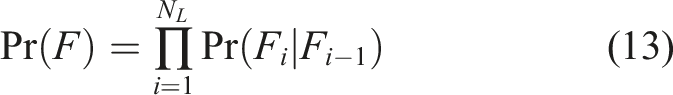
Subset simulation, proposed by Au and Beck (Au and Beck, 2001), is a sequential Monte Carlo method for solving the structural reliability problem and calculating the probability of failure. It is based on the insight, that the failure event F can be expressed as an intersection of N
L
intermediate nested events, where:


The probability of failure can thus be written as a product of conditional probabilities:
During the algorithm, the threshold values b
i
are chosen so that the conditional probability Pr(F
i
|Fi−1) for all but the last intermediate event is fixed to p0. The conditional probabilities of the intermediate events are thus much larger than Pr(F):

The threshold of the last subset level is
This idea of expressing the failure event as an intersection of a sequence of nested intermediate events enables a sequential sampling-based approximation of Pr(F). This approximation has three steps: (1) Draw samples (2) On each subset level i corresponding to an intermediate event F
i
, N
S
samples (3) On the last subset level N
L
the number of samples
From the probability Pr(F), the model evidence is estimated according to equation (10). In addition, samples of
One of the most performance-crucial issues in the BUS approach is the choice of the scaling constant c.
To alleviate this inefficiency, the adaptive version of BUS, aBUS, adapts the scaling constant h
C
= ln(c−1) at every subset level i to the largest value of the likelihood function evaluated for the samples

Algorithm 1 shows the basic aBUS approach. Input: • p( • • N
S
: Number of samples per subset level • N
P
: Number of desired samples of the posterior distribution; usually the same as N
S
• p0: Fixed conditional probability for intermediate events F
i
; Note, that the number of samples N
T
= p0 ⋅ N
S
below the thresholds b
i
of the subset levels must be an integer. Output: • c
E
: Estimate of the evidence • (1) Initialization Augment the parameters Formulate limit state function h( Draw N
S
initial samples Set the scaling constant h
C
to the maximum of the log-likelihood function of the initial samples. Set the initial threshold to b0 = ∞ and the counter variable i = 0 (2) Subset iteration while b
i
> 0: Increase counter by one: i = i + 1. Determination of the threshold b
i
and seeds • Set the threshold b
i
so that p0 ⋅ N
S
of the samples fulfil h( • If b
i
≤ 0, set b
i
= 0. • Count the number N
T
of samples with the limit state function h( • Set Pr(F
i
|Fi−1) ≈ N
T
/N
S
, which for b
i
> 0 is Pr(F
i
|Fi−1) = p0. Generate samples conditional on domain Fi−1 by: • Randomize the ordering of the seeds • Take the N
T
seeds Update the value of the scaling constant. This is the key step of the adaption in aBUS. For a detailed derivation, see (Betz et al., 2018b): • Set the (possibly) adapted scaling constant to • Modify the threshold level to • Set Decrease the dependence of the k = 1…N
S
samples • Draw • Set (3) Post-processing: Set N
L
= i. The posterior samples are the samples Estimate Evaluate the evidence as c
E
= exp(h
C
) ⋅Pr(F).
When choosing the value of p0, one has to consider a trade-off between efficiency, which is expressed as the total number of likelihood evaluations, and the approximation errors in the results of the algorithm. A choice of p0 = 0.1 is “close to the optimum in many cases” (Betz et al., 2018b). Note that there are also approaches which adapt p0 for each intermediate event (Blandfort, 2021).
In addition to selecting the conditional probability of the intermediate events p0, the number of samples N S per subset level must be chosen. N S ≥1000 is recommended (Betz et al., 2018b).
Adaptive conditional sampling in standard normal space
To generate samples conditional on each intermediate event Fi−1 is to draw samples on each subset level F
i
conditional on the previous level Fi−1. Specialized Markov chain Monte Carlo (MCMC) methods are employed which use the existing samples conditional on Fi−1 as seeds of the individual MCMC chains. This procedure ensures that the generated samples are distributed according to p(
The main component of the algorithm is the transition from the current sample Input: • • • • T: Transformation from the domain • intermediate failure domain Fi−1, given by the limit state function h( Output: • • • α(k): indicator of acceptance of sample k, as boolean or integer variable. (1) Sampling of a candidate Draw a candidate sample • Sample Transform candidate sample to physical domain: (2) Acceptance/Rejection If • Set • Set • Set α(k) = 1 Else: • Set • Set • Set α(k) = 0
The choice of the spread of the proposal distribution, which is expressed in terms of s
q
, is crucial for the algorithm’s efficiency. When the spread is large, that is for small s
q
, the candidate samples
An implicit measure of the dependence of the samples, and thus of the efficiency of the algorithm, is the acceptance rate α as the ratio of accepted candidate samples to the total number of candidate samples (Betz et al., 2018b). For subset simulation, α* = 0.44 is suggested as an optimal acceptance rate (Papaioannou et al., 2015). Betz et al. (Betz et al., 2018b) investigate acceptance rates for aBUS with case studies and suggest that values between 0.3 ≤ α ≤ 0.5 are efficient.
In the conditional sampling algorithm 2, the acceptance rate depends on the spread of the proposal distribution, which depends on s q . It is impossible to select the optimal spread of the proposal distribution before evaluating the samples. Papaioannou et al. (Papaioannou et al., 2015) suggest adaptively adjusting the spread of the proposal distribution during the simulation to meet the optimal acceptance rate α*.
This is achieved as follows: A number i = 1, …, N A of adaptions is performed while generating the MCMC chains. The adaption consists of step-wise adjusting the parameter s q of the proposal distribution.
A starting value for the spread parameter

In each adaption step, N
C
chains are generated. For each of these chains, the acceptance rate is calculated. The average acceptance rate
The number N
C
of chains considered for adaption, should be selected such that there are 5 to 10 adaption steps, which can be calculated as N
A
= p0 ⋅ N
S
/N
C
(Papaioannou et al., 2015). Algorithm 3 implements the adaptive version of conditional sampling. Input: • N
S
: Number of samples to be drawn. • N
C
: Number of chains to consider for each adaptation. • • cq,init: Initial scaling parameter, optional. • • α*: Target acceptance rate. Output: • • cq,last: Scaling parameter of the last adaption (1) Initialization For each dimension j of the parameter space, choose an initial spread parameter Calculate the number of adaptions N
A
as the integer division of (N
S
div N
C
) (2) Iterative Sampling for adaption steps i = 1, …, N
A
: For each c ∈ 1, …N
C
of the chains: • Calculate seed index as k = (i − 1)N
C
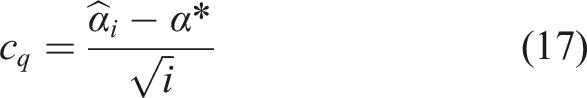
+ c. Take the seed For the states generated with the N
C
chains, evaluate the average acceptance rate Compute the scaling parameter c
q
based on equation (17). Update the spread parameters (3) If there is a remaining number of chains (N
S
mod N
C
) repeat step 2.i. (4) Return the generated samples
Failure-robust parallelization of aBUS
In the application of the aBUS methodology for Bayesian updating, a substantial number of likelihood evaluations are necessitated. A key observation is that some of these evaluations are independent of one another, enabling the parallelized execution. Specifically, within the aBUS algorithm, the likelihood evaluations for the initial samples (as outlined in Step 1.iii) are independent. Similarly, in the aCS algorithm, the generation of Markov chains (referenced in Step 2.i) during the adaptation phases can also be conducted independently.
The analysis of engineering models typically involves the use of complex software systems. Running multiple instances of these systems in parallel, especially when interfaced with external control libraries, may lead to crashes due to resource over-utilization and communication-related issues between the software and the controlling scripts. We experienced crash rates α c of up to 0.5%. This presents a challenge for the parallelization of the aBUS and aCS algorithms. To address this issue, our approach permits these crashes while keeping track of the samples of the failed analyses. This strategy allows for the subsequent re-execution of these analyses, effectively managing the instability without compromising the integrity of the overall analysis.
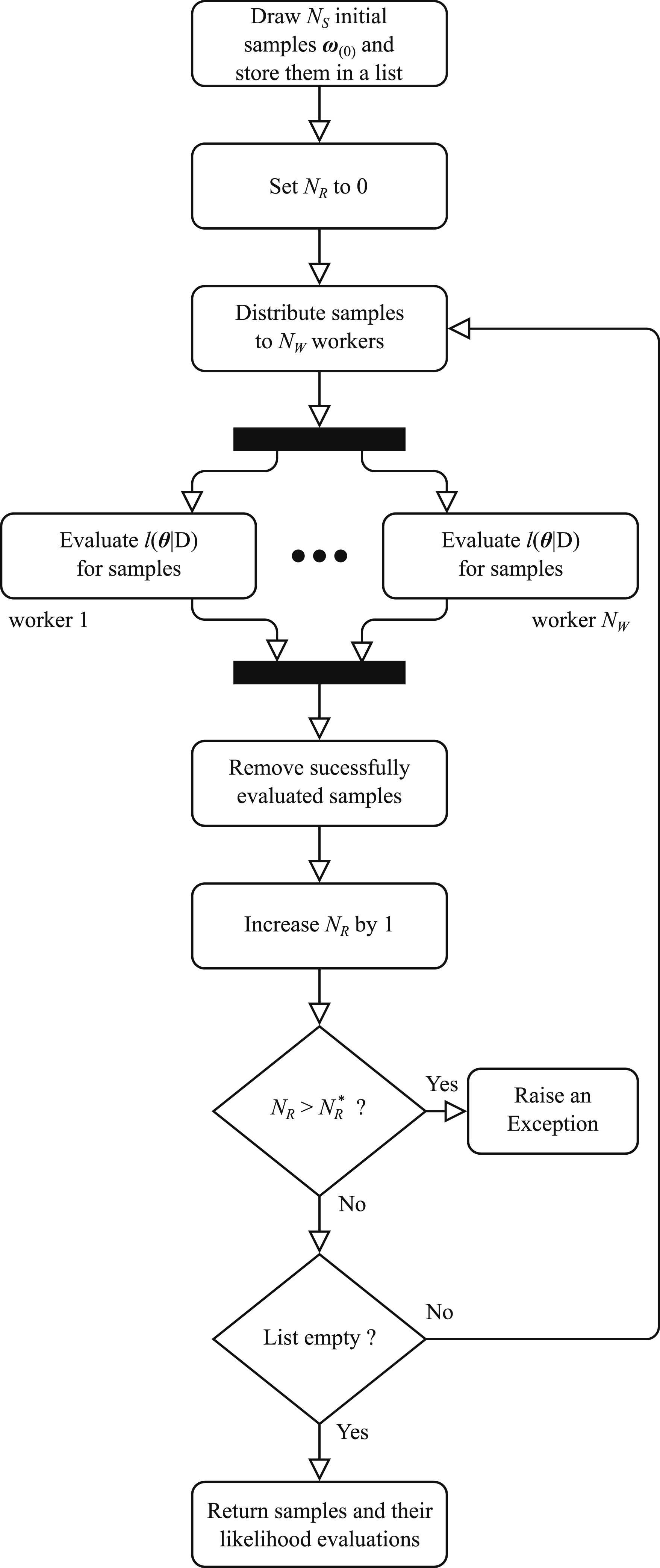
We integrate strategies of parallel execution and crash-handling for a failure-robust parallelization of the aBUS and aCS algorithms. First, Step 1.iii in the algorithm for aBUS is parallelized. The maximum number N
W
of parallel processes is equal to the number of samples N
S
. Figure 1 shows a flowchart of this algorithm, as described in Algorithm 4. Input: • N
S
: Number of samples per subset level (this equals the number of initial samples). • • p( • Output: • • (1) Initialization Draw N
S
initial samples (ii) Set the counter variable N
R
of retries to 0. (2) Iterate, while the list L
S
of samples to be evaluated is not empty and Parallelly evaluate the log-likelihood function Remove the samples from the list that were successfully evaluated. Increase N
R
by 1. If (3) Return the initial samples and the corresponding evaluations of the log-likelihood function, or raise an exception if Flowchart of algorithm 4: Robust parallelization for Step 1.iii in the algorithm for aBUS.
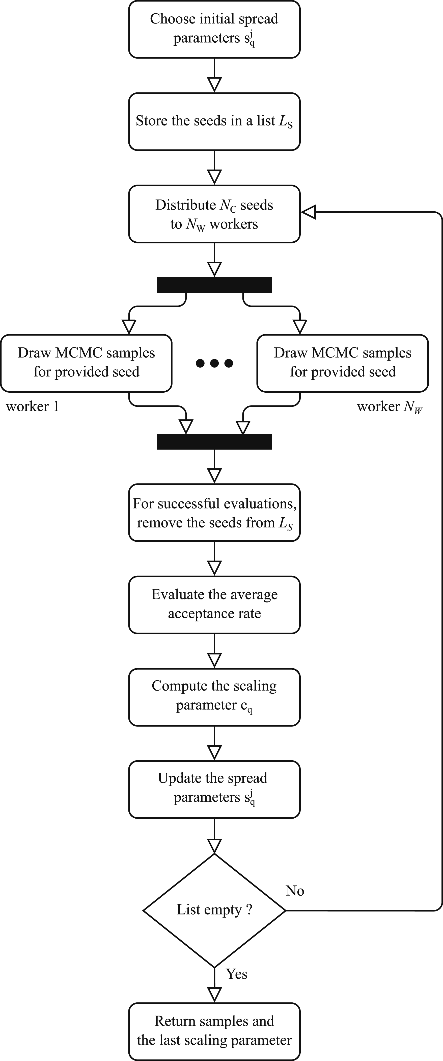
Secondly, the generation of Markov chains in the algorithm for aCS (Step 2.i) is parallelized between the adaptions of Input: • N
S
: Number of samples to draw • N
C
: Number of chains to consider for each adaptation • • cq,init: Initial scaling parameter, optional. • • a*: Target acceptance rate Output: • • cq,last: Scaling parameter of the last adaption (1) Initialization For each dimension j of the parameter space, choose an initial spread parameter Store the seeds from the previous subset level (2) Batch-wise parallel sampling while the list of seeds is not empty: Take N
C
seeds from the list L
S
and use algorithm 2 for conditional sampling in parallel with N
W
worker processes to generate states of a Markov chain. Keep track of which seeds the generation of a Markov chain failed and note the acceptance indicator α(k) of each generated sample. Remove the seeds for which the conditional sampling suceeded from the list L
S
of seeds. Evaluate the average acceptance rate Compute the scaling parameter c
q
based on equation (17). Update the spread parameters (3) Return the generated samples Flowchart for algorithm 5: Robust parallelization for Step 2.i in the algorithm for adaptive Conditional Sampling.
Case study: Vibration-based system identification of the Maintalbrücke Gemünden
The purpose of this case study is to demonstrate the feasibility of updating large engineering models using sampling-based Bayesian updating. To this end, a linear-elastic dynamic structural model of a large railway bridge is parametrized by several uncertain parameters. Their probabilistic distribution is learned based on modal property data.
The bridge
The Hanover-Würzburg high-speed railway line built in the 1970/80s crosses the Main valley near Gemünden am Main, approximately 70 km east of Frankfurt. At the request of the infrastructure owner Deutsche Bahn, the engineering consultancy Leonhardt, Andrä und Partner revised the initial design for the viaduct (Leonhardt, 1986) and proposed a rigid frame bridge with v-shaped piers for the main bridge instead of a tapered three-span continuous girder bridge. In the following, the approach viaducts are not considered and the term “Maintalbrücke Gemünden” is used synonymously for the main bridge across the river, which is shown in Figure 3. Picture of the Maintalbrücke Gemünden spanning over the river Main.
The superstructure acts primarily as a continuous girder with variable spans. The v-shaped piers reduce the main span from 135 m to 105 m. However, the system is semi-integral because the v-shaped piers are joined monolithically to the girder. The cross-section was designed as a box girder with variable heights ranging from 4.5 m to 6 m. A special feature of the structure are the concrete hinges at the bottom of the v-shaped piers, which are among the most heavily loaded of their kind (Schacht and Marx, 2010). Along the box girder, transverse bulkheads are located above the v-shaped piers and at both ends of the box girder.
The data
A permanent monitoring system has been installed on the bridge for research purposes. The system records data during most train passages and twice per day for longer periods. Summary statistics of the measured quantities are aggregated every 30 s. The measured quantities are strains, temperatures, inclinations, accelerations, and vibration velocities. In this contribution, we utilize vibration velocity data recorded with geophones, whose layout is shown in Figure 4. There are 13 vertical geophones distributed along the longitudinal axis of the bridge, which are placed on the floor of the box girder at the western side. Additional geophones are placed on the floor of the box girder at the eastern side to capture torsional mode shapes. Elevation of the bridge with the sensor layout of the geophones.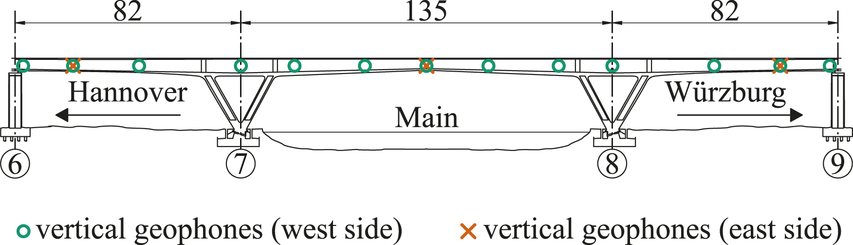
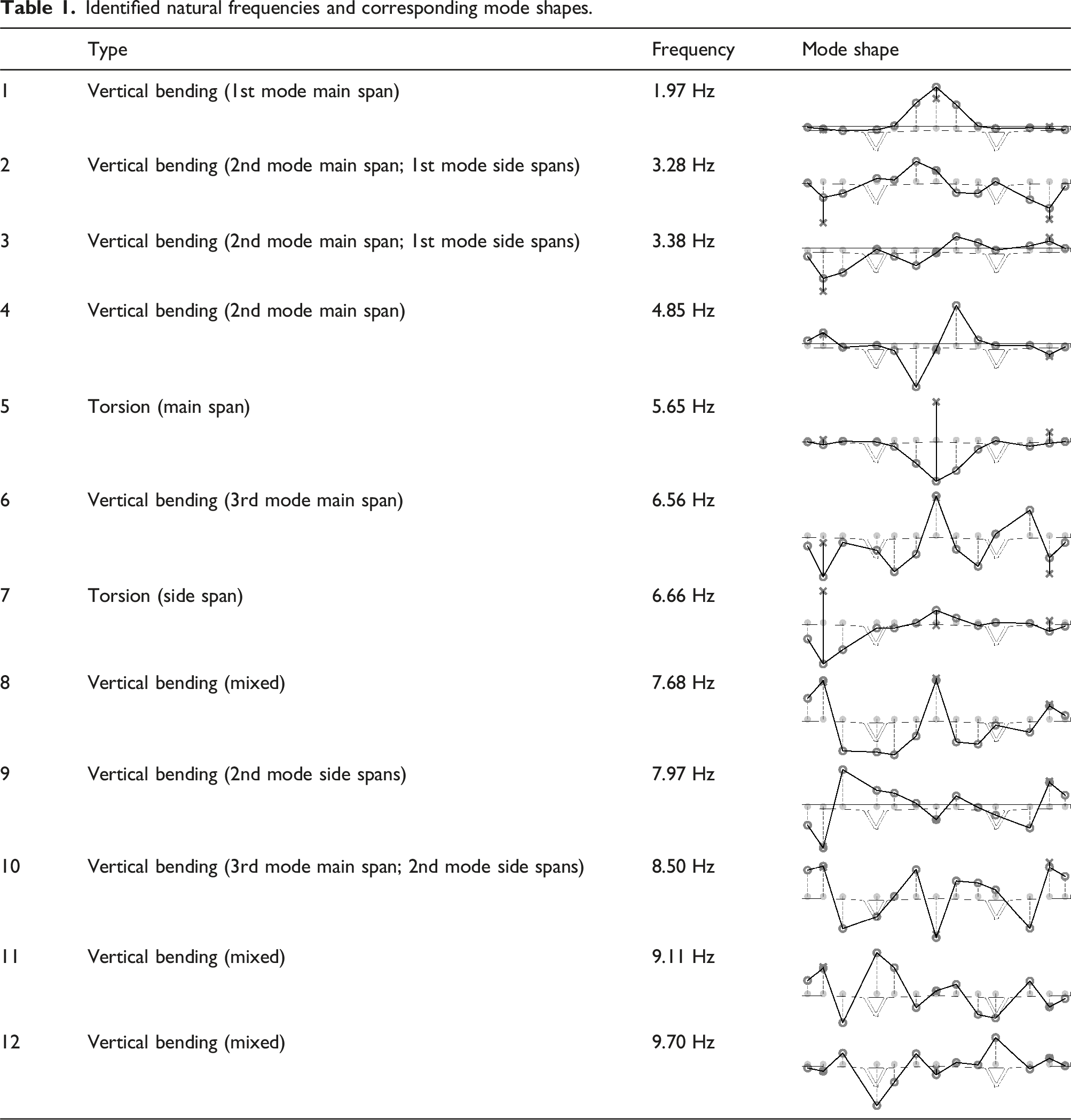
Identified natural frequencies and corresponding mode shapes.
The model
The bridge was represented by a linear-elastic finite-element (FE) model, which primarily consisted of shell elements. The model was defined based on as-built drawings. Based on these drawings, the box girder was partitioned into 86 sections with different geometries. Preliminary investigations showed that the main girder alone could not explain the high torsional stiffness. Therefore, the bridge caps were modelled as additional beam elements and coupled to the outer edges of the main girders. Additional beam elements were connected to the top of the main girder with springs to represent the train tracks. In this way, a moving static load could be applied to the model. The results of this analysis were compared with deformation data recorded during load tests to validate the model (Simon et al., 2022).
Solid elements were used to model the massive blocks of concrete at the bottom of the v-shaped piers which transfer the loads to the concrete hinges. The supports on the piers at both ends of the bridge and the concrete hinges were modelled with spring elements that have a high stiffness for translational degrees of freedom (DOF) but a low stiffness for rotational DOF.
Figure 5 shows the resulting model with 87,180 DOF and highlights the described modelling details. The parameters of the FE model whose probabilistic distribution is updated (see next section) are also indicated in the figure. The rationale for selecting these parameters is as follows: The five sections of the superstructure with different elastic moduli correspond to the main sections produced during the construction of the bridge. To accommodate the aforementioned effect of the bridge caps, their density, elastic modulus, and stiffness of the shear connection were included as uncertain model parameters. The track mass was also considered as an uncertain model parameter. Thus, the masses of the various non-loadbearing members are approximately captured by both the track mass and bridge cap density. The mode shapes in Table 1 indicate that the bearings exhibit some flexibility. Therefore, they were modelled as spring elements that could be parametrized. Overview of the finite element model of the bridge, including parameters.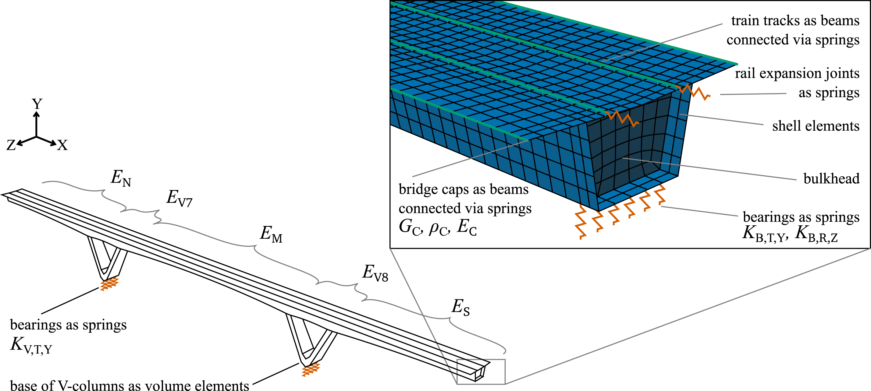
Three probabilistic model classes were formulated: one (referred to as M1) which includes the stiffness KV,T,Y of the spring elements at the bottom of the v-shaped piers as a deterministic parameter with a value of 1012 N/mm, a second one (referred to as M2) which includes this stiffness as an uncertain parameter, and a third one (referred to as M3) which also includes the stiffness KV,T,Y but models the standard deviation of the prediction error as a deterministic parameter with a value of 0.15.
These three model classes are defined to demonstrate the process of model class selection. In essence, this process can be used to determine the most plausible way of modelling the system which includes the selection of the parameters considered in the model updating. The issue of choosing the relevant model classes from the space of possible model classes remains an open research area. For a current discussion, the reader is referred to (Simon et al., 2024).
Model updating
As a basis for updating the structural model, the prior probabilistic model of the parameters is defined and the likelihood function containing the structural model is formulated. These two (the prior probabilistic model and likelihood function) form a probabilistic model class which can be updated with Bayesian updating. The results are shown subsequently.
Formulation of the likelihood function
The likelihood function is formulated based on the prediction error
In this contribution, we define a mode as a pair (
There can be more model-predicted modes than observed modes. Also, the sequence of natural frequencies 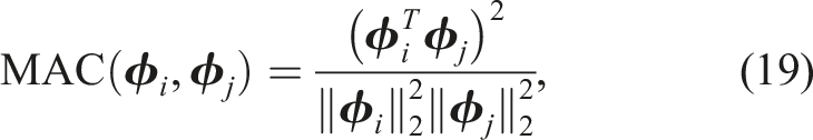
The discrepancy δ
ij
between an observed mode 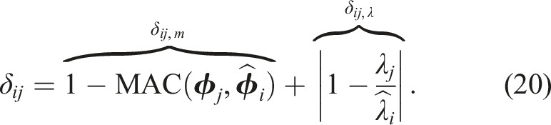
Mode pairing algorithms must seek to match the corresponding predicted and observed modes even when there is a difference in the eigenvalues and mode shapes. At the same time, modes that bear some similarity but do not correspond to each other, such as closely spaced modes, must not be matched.
Our proposed algorithm (as shown in Algorithm 6) addresses these requirements by: (1) sequentially matching the best-fitting pair and removing them from the pool of candidates, and (2) defining a threshold δ* on the discrepancy δ
ij
above which no modes are paired. The first part supports correct matching even when closely spaced modes are present. The definition of the threshold δ* prevents the matching of unrelated modes. Input: • δ*: Threshold value for maximal discrepancy • • Output: • L
P
: list of pairs of observed and predicted modes. (1) Initialize an empty list L
P
= [] for modal pairs. (2) Calculate the discrepancy matrix (3) While the matrix • Find the entry with the lowest discrepancy δ
ij
. Record the indices i* and j* of the corresponding observed and predicted mode. • Append the pair (i*, j*) to the list L
P
. • Delete row i* and column j* from the matrix (4) Return the list L
P
of matched pairs of modes.
With this procedure, we can now align observed and predicted modes. This is the prerequisite for constructing prediction errors
The usage of the mode shape discrepancy δij,m assumes that even if two physical modes are close in frequency, they can be separated by their mode shapes. This implies that the mode shapes are orthogonal. Provided that the spatial resolution of the measured degrees of freedom (DOFs) is sufficient, bridges and buildings typically satisfy this condition. However, in quasi-axisymmetric structures, such as towers, special consideration is required for the modal identification. This is discussed in more detail in references (Au et al., 2021; Jonscher et al., 2023).
The available data
The predicted modes result from an eigenvalue analysis, which is performed based on the deterministic linear-elastic structural model, which is denoted as
There are different ways to model the prediction error of eigenvalues (or, likewise, frequencies), for example, additive (Behmanesh et al., 2015; Behmanesh and Moaveni, 2016; Huang et al., 2019; Simoen et al., 2015) or multiplicative (Koune et al., 2023; Ntotsios et al., 2009) formulations. The eigenvalues have different magnitudes. When the prediction error is modelled as multiplicative, the order of magnitude of the prediction error is independent of the order of magnitude of the eigenvalue. This formulation is thus deemed more suitable. It can be expressed as the ratio of predicted and observed eigenvalues. Taking the logarithm of this ratio yields the same order of magnitude of the prediction error, regardless of the order of magnitude of the numerator and denominator in the ratio (Simon et al., 2020). In this contribution, we define the prediction error for one eigenvalue of a matched mode with index m as:
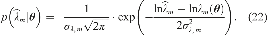
Due to the modelling choices of the current contribution, the prediction errors of different modes are statistically independent conditional on a realization of σ
λ
, so that for all modes m: σλ,m = σ
λ
. The standard deviation σ
λ
of the prediction errors of the eigenvalues is modelled as uncertain parameter and are thus included in the parameter vector 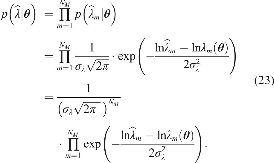
The likelihood function 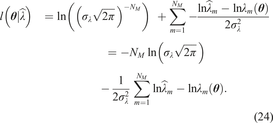
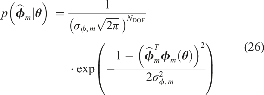
To formulate a likelihood function based on the prediction errors of the mode shapes, we adopt a vector-valued additive prediction error model as introduced in (Beck et al., 2001):
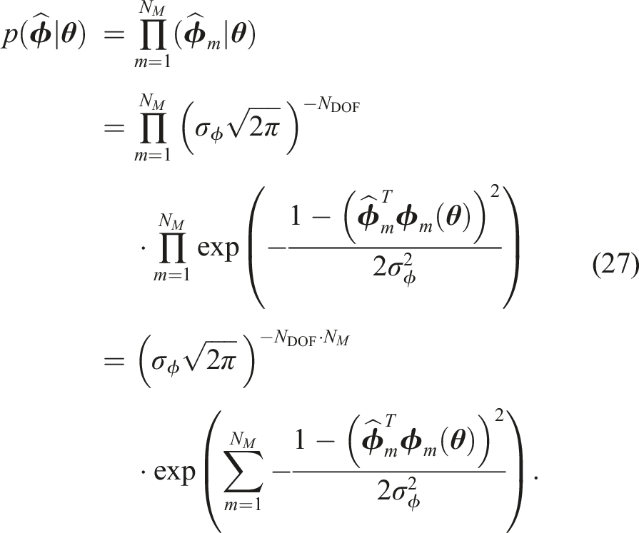
When 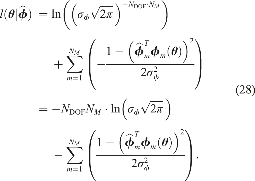
The joint probability density of the observed data 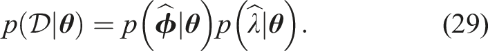
The log-likelihood function 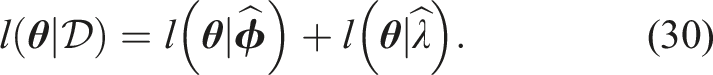
By constructing the likelihood function in this way, the statistical dependence among the observations of the identified modal eigenvalues
Prior probabilistic model of the parameters
The parameters of each stochastic model class are modelled as random variables. The prior marginal distributions of the different model parameters are derived from the literature (Fédération internationale du béton, 2013; Joint Committee on Structural Safety (JCSS), 2001), design documents, and engineering judgment.
Prior marginal distributions of parameters defined in terms of distribution type and parameters.
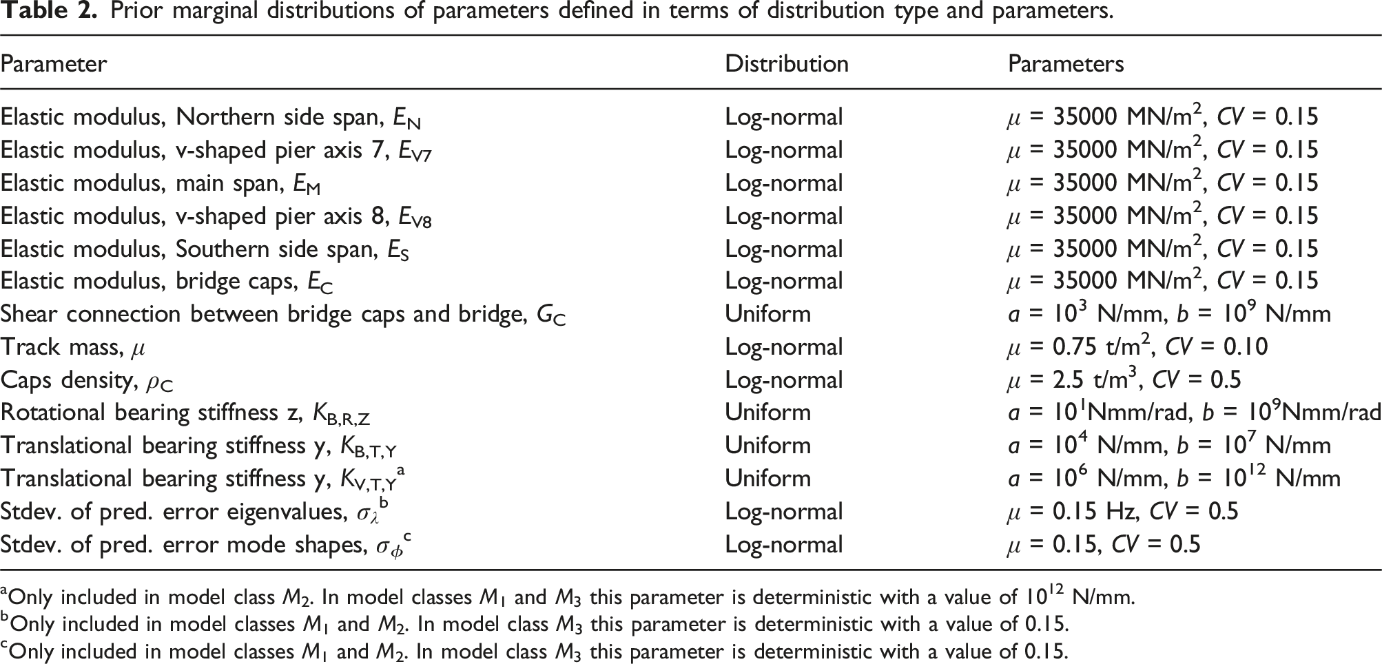
aOnly included in model class M2. In model classes M1 and M3 this parameter is deterministic with a value of 1012 N/mm.
bOnly included in model classes M1 and M2. In model class M3 this parameter is deterministic with a value of 0.15.
cOnly included in model classes M1 and M2. In model class M3 this parameter is deterministic with a value of 0.15.
Alternatively, global sensitivity analyses can be performed to identify the relevant parameters to be considered in the model updating (Brownjohn et al., 2001; Jang and Smyth, 2017). This approach is, however, outside the scope of this case study.
Results
Model updating with parallelized aBUS was performed based on the three described model classes M1, M2, and M3 and the identified modal property data. The updating was performed on an AMD Ryzen 7 PRO 5750G CPU with eight physical cores. A sample size of N S = 4000 and a conditional probability for subset simulation of p0 = 0.05 were used as settings for aBUS and a total of N W = 10 worker processes were utilized. The computation times were 26 h, 18 h, and 23 h. Model updating provided the posterior samples of the parameters and an estimation for the evidence. The evidence is used for model class selection. Based on the posterior samples, we can update the probabilistic predictions of the model output.
Model class selection
For each postulated model class M
i
, using i ∈ {1, 2, 3}, the evidence
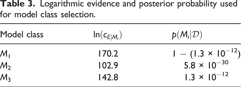
Logarithmic evidence and posterior probability used for model class selection.
Posterior parameter distributions
The prior and posterior (empirical) marginal distributions of the parameters influencing the stiffness of the main girder are shown in Figure 6. In general, the posterior distributions are more narrow and shift to higher values. Prior and (empirical) posterior marginal distributions of the stiffness-related parameters of the elastic moduli of the Northern side span, EN, the v-shaped pier axis 7, EV7, the main span, EM, the v-shaped pier axis 8, EV8, the Southern side span, ES, and the bridge caps, EC.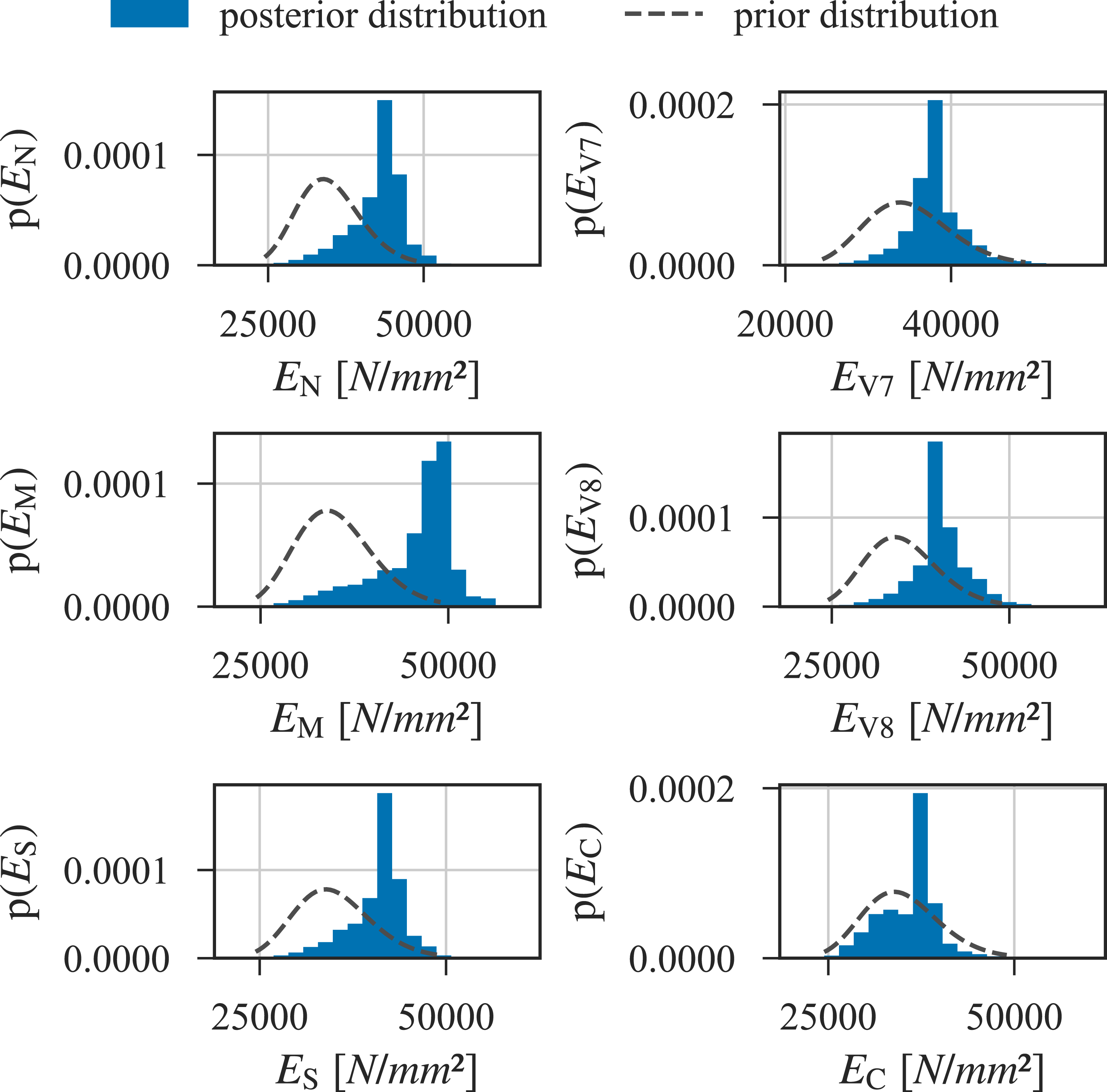
The prior and posterior (empirical) marginal distributions of the parameters governing the mass of the bridge are shown in Figure 7. The posterior distribution of the track mass shifts slightly to lower values, while the distribution of the density of the cap material shifts significantly to lower values. Prior and (empirical) posterior marginal distributions of the mass-related parameters: track mass, μ and caps density, ρC.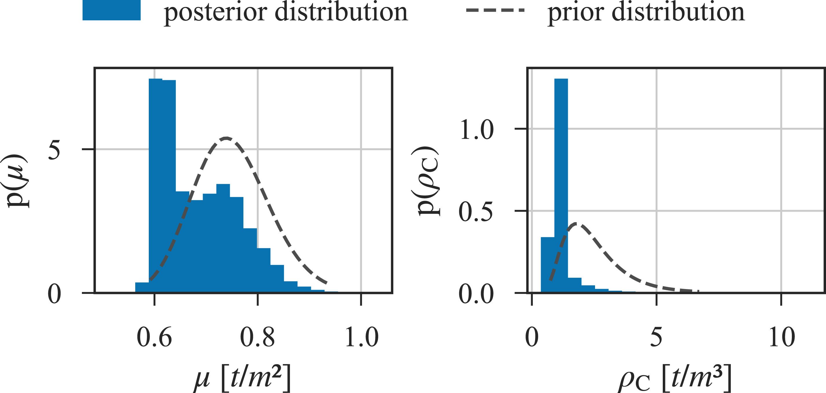
The prior and posterior (empirical) marginal distributions of the parameters related to the springs are shown in Figure 8 on logarithmic scales. No significant change is observed for the shear connection and rotational bearing stiffness. The posterior distribution of the stiffness of the translational springs shifts to higher values. Prior and (empirical) posterior marginal distributions of the parameters related to springs: The shear connection between bridge caps and bridge, GC, the rotational bearing stiffness z, KB,R,Z, and the translational bearing stiffness y, KB,T,Y.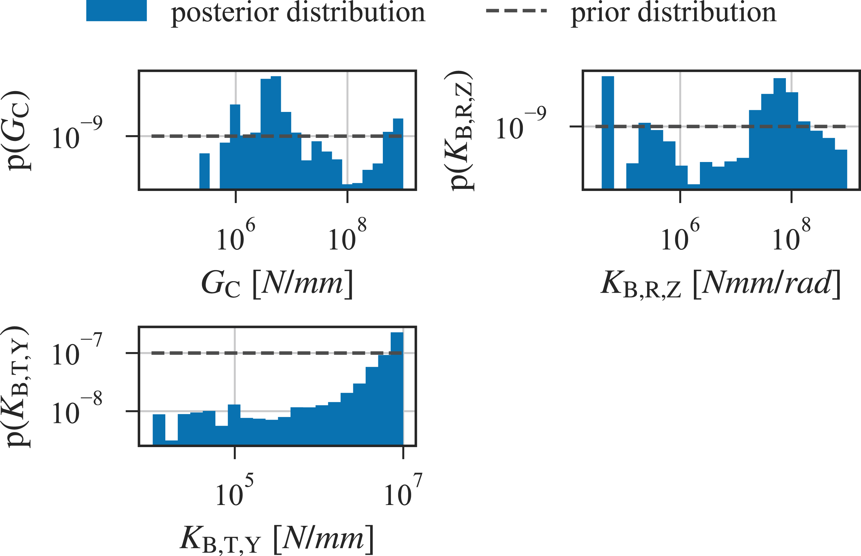
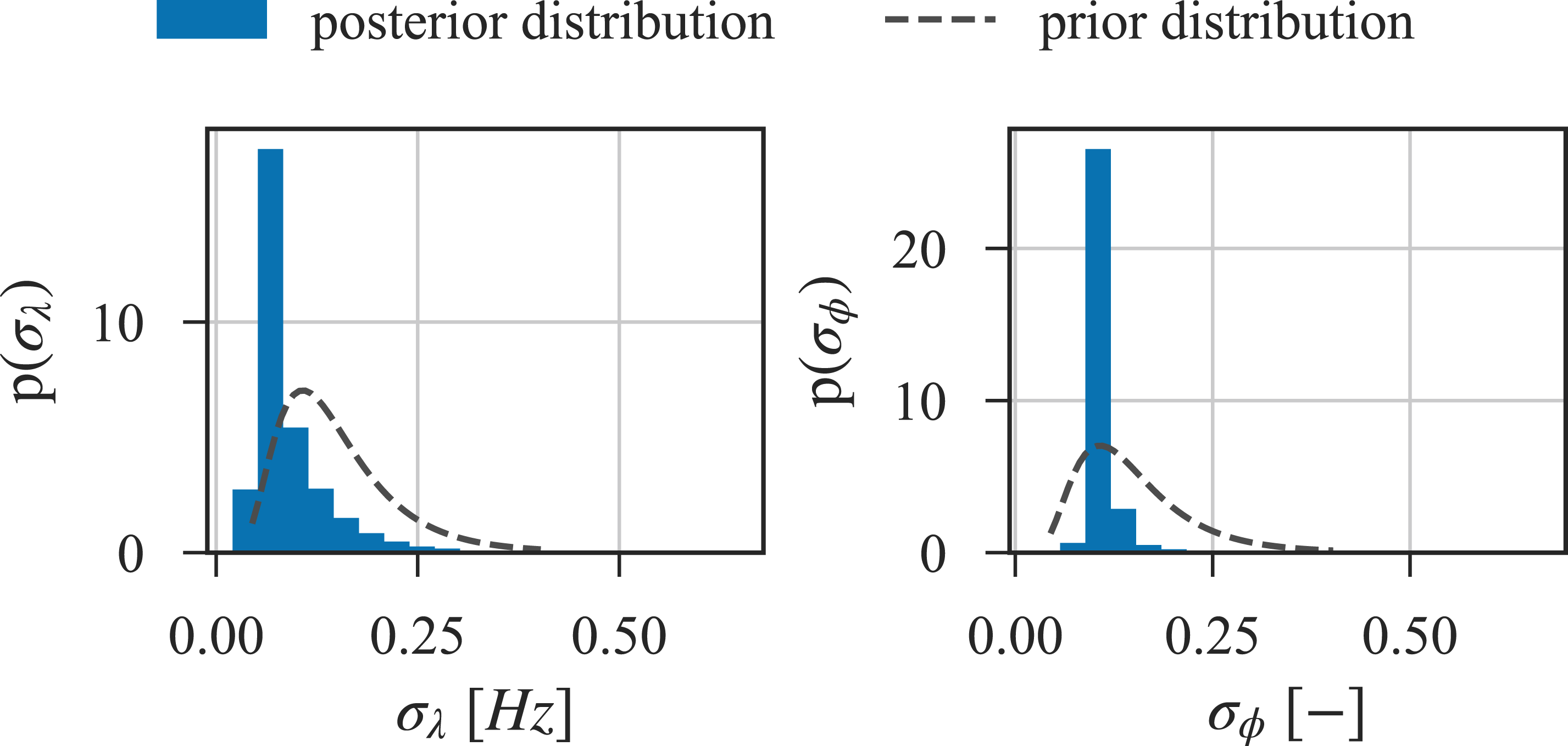
The prior and posterior (empirical) marginal distributions of the parameters related to the standard deviation of the prediction errors are shown in Figure 9. There is no change in the standard deviation of the prediction errors of the eigenvalues, but the uncertainty of the standard deviation of the prediction errors of the mode shapes significantly reduces due to the model update. Prior and (empirical) posterior marginal distributions of the parameters related to errors: The standard deviation of the prediction errors of the eigenvalues, σ
λ
, and the standard deviation of the prediction errors of mode shapes, σ
ϕ
.
Model predictions
One goal of model updating (e.g., in a digital twin framework) is to obtain improved model predictions. One way to evaluate the quality of model updating is to evaluate and compare the model predictions based on prior and posterior parameter distributions. For this purpose, 4000 samples of each of the prior and posterior parameter distributions were used to predict the modal properties of the bridge. These results were matched with the observations based on the same logic as described in Algorithm 6 and equation (20).
Comparison of prior and posterior predictions with observed modal properties.
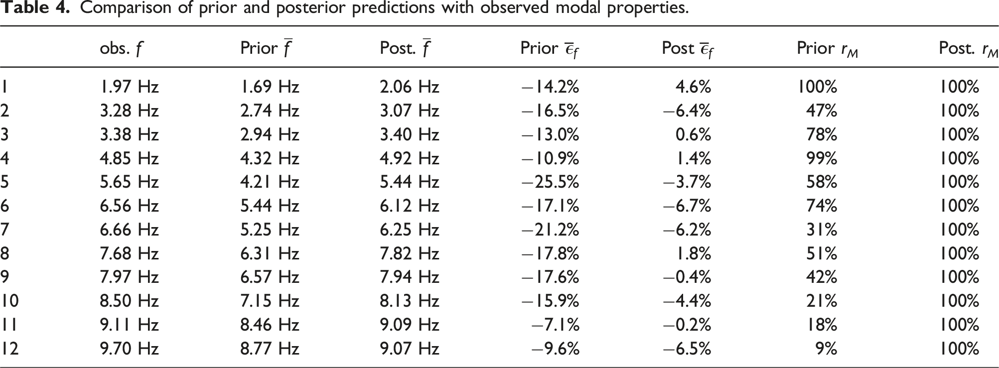
Figure 10(a) and (b) show the matrices of the average MAC values between predicted and observed mode shapes. The average MAC values of some observed modes with both prior and posterior predicted modes are quite low. One hypothesis is that the observed mode shapes are not well identified based on the available vibration velocity data, which result from ambient excitations. The illustrations of the mode shapes in Table 1 also supports this observation. Comparison of MAC values. (a) Matrix of the mean MAC value of the prior predicted modes versus the observed modes. (b) Matrix of the mean MAC value of the posterior predicted modes versus the observed modes. (c) Mean MAC values between the identified modes and the prior and posterior predictions and range of MAC values between the identified modes and the other observations.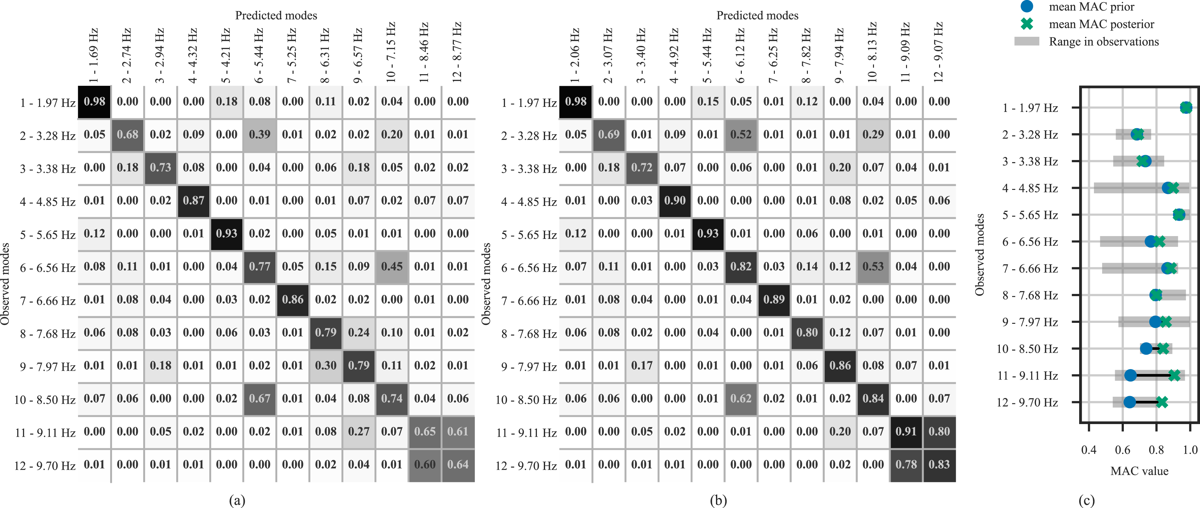
To examine this hypothesis, the modes identified in the current dataset were compared to those of 11 other datasets. The MAC values of these comparisons show significant variations, further supporting this hypothesis. Figure 10(c) relates the average MAC values between the identified modes and the predicted ones to the range of MAC values between the identified modes and the other 11 observations. For some modes, there is very little congruence between observations with a lower bound of MAC values as low as 0.4.
From a system identification perspective, this result is unsatisfactory and requires further examination. For the model updating the upper bound of the range of MAC values between observations also indicates the upper bound for a plausible accordance between the posterior predictions and the identified modes. It would be implausible for the predictions to match the identified modes better than other observations. Figure 10(c) also shows improvement of the posterior predictions in comparison to the prior predictions.
Performance analysis
The motivation for this work is to provide efficient Bayesian Updating of engineering models by parallelizing aBUS. Theoretically, the reduction in execution time of the improved algorithms presented in this contribution would scale (almost) linearly with the number of processes used. However, the execution time depends on other factors, such as the synchronization of intermediate results, bottlenecks like time-consuming input-output operations, and the constraints imposed by the hardware, operating system, and engineering software used. This observation leaves us with the question of how the parallelized algorithms scale in practice.
In computer science, the performance of parallel programs can be analysed with appropriate measures of measured execution times (Rauber and Rünger, 2010: Chapter 4). To examine our case, we use the performance measure speedup S, which evaluates the reduction in execution time T of a program executed in parallel on N
W
worker processes compared to the sequentially executed program as:
The achievable speedup can be expressed by Amdahl’s law (Amdahl, 1967), which assumes that a fraction f
S
, 0 ≤ f
S
≤ 1, of the program must be executed sequentially and the rest 1 − f
S
can be executed in parallel. The execution time T(N
W
) of the parallelized program consists of the time of the sequential part and the parallelizable part: T(N
W
) = f
S
⋅ T(1) + (1 − f
S
)/N
W
⋅ T(1). The achievable speedup is thus (Rauber and Rünger, 2010: 164):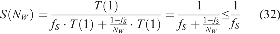
In this contribution, we examine the parallelized variant of aBUS with the case study from the previous section as a real application benchmark. This real application benchmark thus depends on the problem, the engineering software used, and the hardware. In this scenario, we try to estimate the fraction f S that must be executed sequentially. This estimate serves as an indicator of the overall performance of the parallelized algorithm.
Bayesian Updating was performed on the model class M2 with the measured data several times. The number N W of worker processes was varied between 1 and 16 and the execution time was recorded. For each N W , three tests were performed. A large variance was observed for repeated executions with the same number of worker processes. This variance can be interpreted by the fact that subset simulation and thus aBUS is a stochastic algorithm by nature, which is prone to performance variations.
To infer probable values for f
S
, Bayesian updating was performed on the benchmark results. The processor used (AMD Ryzen 7 PRO 5750G CPU) has eight physical cores. The performance law for N
W
is likely to be different above and below the number of physical cores. Therefore, only benchmark data with N
W
≤8 was used. For each test, the speedup was calculated with respect to the average sequential time Speedup over the number of worker processes. The speedup observed in the benchmark tests is shown as dots. The prediction of speedup by Amdahl’s law with the inferred parameter f
S
is shown with mean and 90% HDI.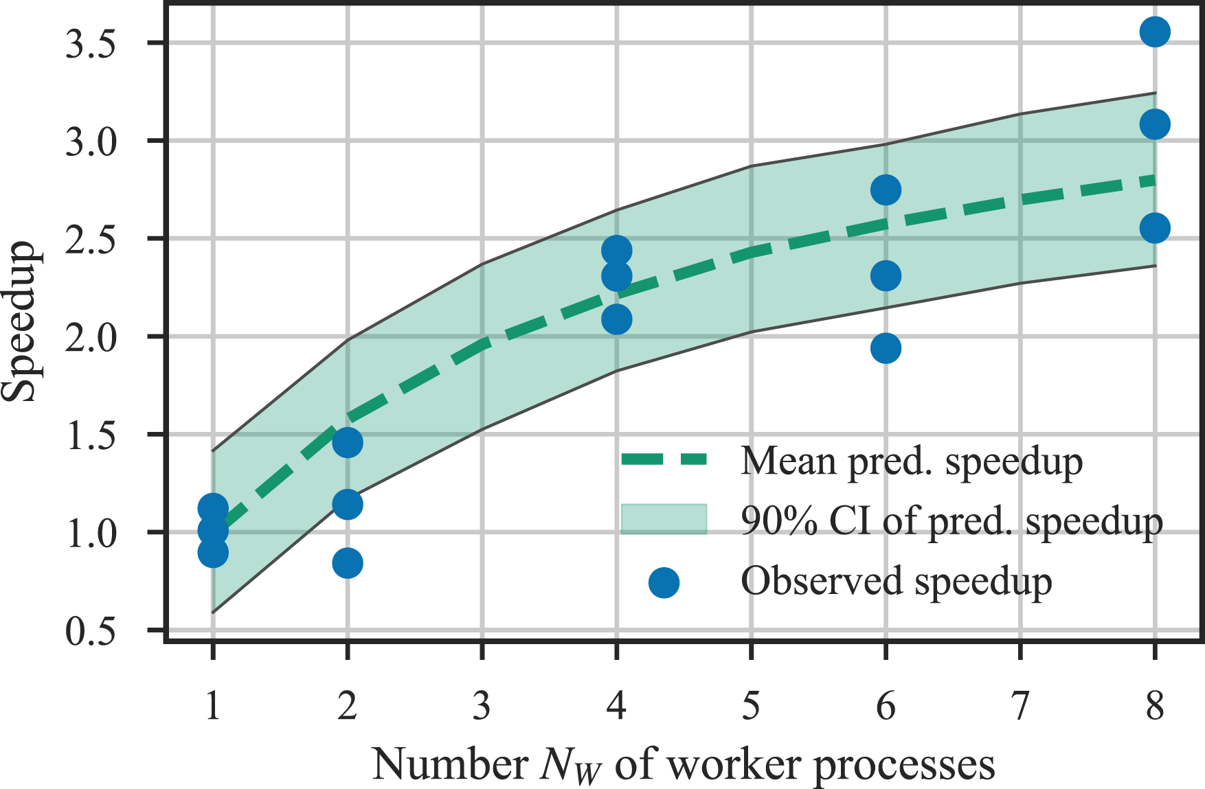
We now know that the expected value of the upper bound of the achievable speedup for the case study is 1/f S = 3.7. This serves as an indicator of the performance of the parallelized algorithms.t
Discussion
This paper shows how sampling-based Bayesian updating of large engineering models with many uncertain parameters can be performed more efficiently, while also providing an estimate of the model evidence. For this purpose, aBUS combined with subset simulation was parallelized and applied in a case study considering a large concrete railway bridge. In the following, we discuss the algorithmic improvements and case study separately.
Algorithmic improvements
The described failure-robust parallelization of two components of aBUS is a straightforward but important improvement of the algorithm. The strengths of this approach include: (1) Enhanced computational efficiency: Parallelization of the aBUS algorithm significantly improves computational efficiency. This is crucial for handling large engineering models with many uncertain parameters, enabling more efficient Bayesian updating. (2) Robustness to computational failures: The design of the parallelization to accommodate and recover from computational failures enhances its robustness.
There is room for improvement in the following areas: • Chain generation robustness: While the generation of Markov chains as a whole is robustly parallelized, a failure in the evaluation of the last candidate sample of a chain might render previous samples ineffective. This is due to the synchronous nature of the algorithm, which evaluates the acceptance rate of a batch of Markov chains to adjust the scaling parameter λ. In scenarios with a high probability of computational failure, this leads to performance degradation. • Limit on the number of worker processes: The number of worker processes (N
W
) of Algorithm 5 is currently limited by the number of chains (N
C
) considered for adaptation, which may restrict the scalability of the algorithm in certain applications. • Influences on scaling parameter adaptation: The adaptation of the scaling parameter λ is influenced by several factors, including the chain length (generally • Leveraging subset simulation research: There is substantial research on subset simulation that offers critiques and improvements (e.g., Blandfort, 2021; Breitung, 2019; Chen et al., 2022; Zhao and Wang, 2022). Integrating insights from this research could further enhance the performance and accuracy of the Bayesian updating process with parallelized aBUS.
Case study
The case study considering the Maintalbrücke Gemünden bridge was conducted to demonstrate and verify the efficiency of the proposed parallelization of aBUS. By applying this approach, large engineering models can be updated within a reasonable time frame.
The approach was verified by comparing the prior and posterior predictive distributions of the modal properties with the observed data. Based on the posterior predictions, more modes could be clustered and thus matched to the observed modes. The mean natural frequency of the predictions was closer to the observed natural frequencies. The average MAC values slightly decreased.
To match the observed modes with the predicted modes, a heuristic mode pairing algorithm was used. The results differ depending on the chosen heuristic. Investigations using distance measures other than the one defined in equation (20) revealed slightly different posterior distributions for the case study presented in this contribution. In addition, the impact of the threshold value δ* on the mode pairing needs to be examined further. The optimal choice of this threshold achieves a trade-off between (a) correctly matching corresponding modes even if the value of the discrepancy δ ij is large and (b) preventing the incorrect matching of closely spaced modes. In a related example (Brehm et al., 2010), the results of a sensitivity analysis varied depending on the measure used for mode shape similarity in mode matching. Further research is needed to compare different possible metrics (Morales, 2005; Vacher et al., 2010) and their limitations. For intrusive methods that have access to the stiffness and/or mass matrices of a finite element model, updating schemes without mode matching exist (Das and Debnath, 2020; Huang and Beck, 2015; Yuen et al., 2006).
A total of twelve well-separated modes were employed for the purpose of model updating. As is the case with other structures, closely-spaced modes require modal analysis methods capable of separating them (Au et al., 2021; Jonscher et al., 2023). The uncertainty arising from measurement uncertainty and uncertainty of the modal identification inform the prior probabilistic model of the prediction errors. An extended approach can include the uncertainties of the modal identification into the model updating process (Au and Zhang, 2016).
Different assumptions about the nature of the prediction errors and their correlation structure lead to different results (Koune et al., 2023; Simoen et al., 2013). Considering these different assumptions has not been part of this case study, but should be included in a more thorough application.
In addition, it is important to consider other modelling choices, such as parameter selection, assumptions about physical laws, and the level of modelling sophistication. Sensitivity analysis is a common practice for identifying candidate parameters for updating (see e.g., Brownjohn et al., 2001; Jang and Smyth, 2017; Moravej et al., 2019; Simoen et al., 2015). However, this practice only considers parameter selection and not other modelling choices. For further discussion on modelling choices for model-based SHM, please refer to (Simon et al., 2024). A decision-theoretic approach for model selection is presented in (Kamariotis and Chatzi, 2023).
The current case study did not consider all three sources of influencing factors in modelling and model updating: mode pairing heuristics, assumptions about prediction errors, and modelling choices. It is crucial to consider these factors in real-world scenarios. Using aBUS in a parallelized manner, it is possible to evaluate these influences based on model class selection.
Performance
The main objective of this contribution is to increase the efficiency of aBUS through parallelization. Therefore, the performance of the parallelized version was compared to the conventional unparallelized aBUS in terms of achieved speedup. The benchmark tests conducted in the case study revealed an expected upper bound of 3.7 for the speedup. Although this is an improvement, it falls short of the expected results when analysing the improved algorithms. The non-parallelizable fraction f S of the execution time that remains is likely to be implementation-specific and/or dependent on other hardware factors besides the number of processes. Therefore, it should be examined in additional applications.
In addition to the speedup, scalability may also be of interest as a performance measure. Scalability refers to how well additional processes improve performance as the problem size increases (Rauber and Rünger, 2010: 165). The motivation for parallelizing is to address Bayesian updating of large engineering models. Therefore, scalability is an important indicator of how well the parallelized algorithms allow for the use of larger engineering models. However, Bayesian updating presents a challenge in defining the problem size, as it could refer to the execution time of the engineering model, the number of random variables, or the number and the variety of observations. Additionally, the problem size is dependent on the formulation of the problem, which is expressed in the probabilistic model class. In engineering structures, the formulation of the problem is determined by the size and type of the structure as well as the sophistication of modelling. As such, the issue of defining the problem size and investigating its effects on the efficiency of the parallelized aBUS approach is beyond the scope of this contribution and requires further examination.
In the case study, a target value of N S = 4000 samples was used to approximate the posterior distribution of the parameters and the model evidence. Fewer samples might also suffice, but the error in the results must be considered (Betz et al., 2018b).
In addition to the parallelization of the sampling, there are three additional possible approaches to improving the efficiency of aBUS (1) optimization of the MCMC sampler used within each subset, as done by Papaioannou et al. (Papaioannou et al., 2015), and Wang et al. Wang et al. (2019), and the optimization of the sampling-related parameters of the algorithm, such as p0 and N S , as done by Betz et al. (Betz et al., 2018b), (2) reduction of model evaluation time by constructing surrogate models, such as artificial neural networks (Giovanis et al., 2017), or adaptive kriging (Wang and Shafieezadeh, 2020, 2023; Yuan et al., 2022, 2024, 2025), and (3) data reduction techniques (Ur Rehman et al., 2016) to remove data with redundant information and thus reduce the number of likelihood evaluations.
Surrogate models bear their own challenges in terms of evaluating trade-offs between different types of surrogate models, (Alizadeh et al., 2020; Bhosekar and Ierapetritou, 2018), robustness in the presence of failed simulations (Palar et al., 2019), validation (Bhosekar and Ierapetritou, 2018; Palar et al., 2019), and accuracy (Alizadeh et al., 2020; Palar et al., 2019).
The current contribution improves the efficiency of aBUS through parallelization and addresses the issue of failed simulations. Future research should consider the combination of parallelization and surrogate modelling.
Concluding remarks
In this contribution, we demonstrate that parallelizing aBUS enables Bayesian updating of a large engineering model within a reasonable time. This is a contribution to the field of model-based SHM and has implications for model updating of large engineering structures in general.
Further research is needed in three areas. First, the proposed method requires control parameters and employs heuristics that influence aBUS, both of which should be subject to scrutiny.
Second, the algorithm improved in this contribution fulfils the aims of efficiency, high-dimensional parameter spaces, and providing an estimate of the model evidence. However, further evaluation is necessary to assess its performance and limitations in these three areas. It is crucial to compare it with other methods, as done by (Smith et al., 2023) in their comparison of sampling-based methods. Such a comparison should include the use of surrogate models. An example of comparing surrogate models as part of structural reliability analyses is provided in (Moustapha et al., 2022).
Third, there are significant gaps between the research on model updating and its adoption by practitioners (Ye et al., 2022). Our contribution lowers barriers to adoption by making Bayesian updating of large engineering models feasible in engineering practice. However, further research is necessary to validate the quality of updated models and their modelling procedures (Simon et al., 2024).
Footnotes
Acknowledgments
The authors would like to express their gratitude to their colleagues at BAM, Bauhaus-Universität Weimar, and Deutsche Bahn for organizing, implementing, and operating the continuous monitoring of the Maintalbrücke Gemünden and conducting the accompanying load tests and unmanned aerial system (UAS) flights (Simon et al., 2022).
Declaration of conflicting interests
The author(s) declared no potential conflicts of interest with respect to the research, authorship, and/or publication of this article.
Funding
The author(s) disclosed receipt of the following financial support for the research, authorship, and/or publication of this article: This work was performed as part of the AISTEC joint research project, which was financially supported by the German Federal Ministry of Education and Research (Bundesministerium für Bildung und Forschung – BMBF) through grant 13N14658 and VDI Technologiezentrum (VDI TZ).
Data Availability Statement
An example implementation of the parallelized version of aBUS is available at: https://zenodo.org/doi/10.5281/zenodo.10948540 (Simon, 2024). This implementation is built upon the excellent Open Source implementation of the Engineering Risk Analysis group of TU München, among which the authors of (Betz et al., 2016, 2018b; Papaioannou et al., 2015; Straub and Papaioannou, 2014).
Likelihood function for mode shapes
In this contribution, we adopt a vector-valued additive prediction error after (Beck et al., 2001):
The scaling constant αm,o is needed to formulate the prediction error for arbitrarily scaled mode shapes. Even if mode shapes are unit-normalized, the mode shape vectors may point in opposing directions. The scaling constant is defined as:
With
Based on the formulation of the prediction error, we can define the probability density of observing a mode shape
The final probability density of observing a mode shape