Sage Journals: Discover world-class research

Abstract

This paper reports an investigation of deep learning techniques in structural damage identification that can overcome the limitations of traditional visual inspection. First, a vibration-based deep learning model is established to locate the damage in a beam and a truss structure. Then an optical photo-based model is established and used to classify different defects. Based on the satisfactory outcomes of these two models, a new structural health monitoring technique is proposed through the infusion of optical photos and vibration data. Vibration signals and true structural images for a truss are used to demonstrate the capability of the proposed method. It was found that the infusion of vibration data and optical photos can enhance damage identification significantly and overcome the drawbacks in the existing deep learning models due to incomplete vibration signals or blurred optical photo inputs.

Keywords

deep-learning vibration damage identification infusion of vibration data and optical photos structural health monitoring

Introduction

Detecting structural damage, such as corrosion and cracks, has always been an essential process in a structural health monitoring system. Cracks in many structures, particularly concrete structures, occur frequently due to changing load conditions. As a result, those cracks are often, if not always, expressed as lines or curved lines with different orientations and intensities, which are typically darker and more connected compared to the original color of a concrete background. In the last several decades, visual inspection, by trained technicians, is the main approach to detect structural damage, which is typically time-consuming and costly. Therefore, instead of using manual visual inspection, researchers are increasingly attracted to computer-vision-based sensors for structural damage detection due to their significant advantages. By using such sensors, image processing processes like edge detection can be conducted using properly prescribed thresholds. Currently, two main image processing methods are used to detect defects in structures, especially for cracks: one is the image binarization method, and the other is the sequential image processing method. Liu (2014) proposed an image binarization method to detect cracks and had satisfactory accuracy. Ebrahimkhanlou (2016) researched the sequential image processing method that was carried out to detect cracks in images of concrete surfaces successfully. However, both methods were based on edge detection algorithms through some filters, such as Roberts, Prewitt, Sobel, and Gaussian (Yang et al., 2018). Usually, these methods are time-consuming and could only detect the existence of cracks on the surface, but they could not evaluate the embedded cracks and classify different types of defects.

To overcome the shortage of vision-based crack detection methods as described above, recently some researchers intended to use emerging deep learning techniques to classify and evaluate structural defects such as cracks and corrosion. Rawat and Wang (2017) adopted a CNN method to classify cracks, spalling, and potholes. Chen and Jahanshahi (2018) proposed a CNN-based crack detection system and used a Naïve Bayes data fusion scheme to extract cracks from the video frames captured for the structure. Dorafshan et al. (2017) proposed a faster CNN model with image binarization to obtain the locations of cracks in the pixel-level precision. Li et al. (2020b) trained and tested a deep-learning model using 6000 tunnel crack images and compared different crack mechanisms. Their model significantly outperformed basic U-net, fully convolutional networks (FCN), SegNet, and multi-scale fusion crack detection (MFCD) for detecting cracks in tunnels through noisy images. Fan et al. (2020), Li et al. (2020a), Soloviev et al. (2019), and Tong et al. (2018) also proposed deep CNN models to find cracks and their lengths and sizes on pavement surfaces.

On the other hand, dynamic characteristics of a structure, such as natural frequency, damping ratio, and mode shape, could also be used for structure health evaluation to identify damages and their locations. This is based on the theory that structural damage would cause a change in the mass and stiffness distributions of structures, leading to a change in dynamic characteristics (Adeli and Jiang, 2018; Al-Qudah and Yang, 2023; Cawley and Adams, 1979). Therefore, vibration-based structural damage detection methods with system identification could build correlations between the vibration features and the damage information (Chang and Kim, 2016; Reynders et al., 2014; Yang et al., 2005), except natural frequencies are not sensitive to minor damages and could be easily contaminated by environmental factors. Following a similar thought process as the image-based structural condition assessment, some researchers also investigated identifying damages through deep learning models with vibration data inputs. Lin et al. (2017) proposed a CNN-based deep learning method, containing six convolutional layers and three maximum pooling layers. This CNN-based system was then trained using the raw vibration data of a finite element beam and the damage was detected successfully with high accuracy (94.57%). Other researchers adopted the CNN-based method and found the damages caused by losing bolts of a steel truss with high accuracy (Avei et al., 2018). Recently, fault images and vibration data have been directly fed to a deep learning model for damage diagnosis (Al-Qudah and Yang, 2024; Mao et al., 2022; Wang et al., 2019).

However, there is a challenge in literature on how to infuse vibration signals and photo images in structural health monitoring. In this paper, a comparison of different deep-learning models using vibration signals and defect photos was conducted separately first, and then a novel hybrid deep-learning model was developed combining the inputs of both vibration signals and defect photos, which results in an improved accuracy of defect identification and classification.

Comparison of different deep-learning models using vibration signals

Deep learning-based damage detection using vibration data

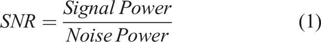
Typically, there are three main sections in a convolutional neural network to identify the structural damage through vibration data at monitoring locations, including (1) dataset collection, (2) CNN model training, and (3) validation and prediction. Vibrations at monitoring locations under dynamic loads are obtained in the ABAQUS model. The collected vibration database was enlarged by adding Gaussian white noises with different Signal-To-Noise ratios (SNR) at different cases using equations (1) and (2) below.

S N R = \frac{S i g n a l P o w e r}{N o i s e P o w e r}

(1)

\begin{array}{l} S N R (d B) = 10 \log_{10} \frac{S i g n a l P o w e r}{N o i s e P o w e r} \end{array}

(2)

Then, the vibration data are classified as different patterns according to different damage cases and are divided into three groups randomly: 70% of which for training, 15% of which for validation, and 15% of which for testing. The training dataset is sent to the proposed CNN model as the input data to train this system. The training section and validating section are necessary for the CNN model to build and improve the sensitivity of the feature learning and the performance of classification. Finally, the test dataset is sent to the model to predict and obtain the accuracy of this model.

The CNN model is proposed to compose of three layers (convolution layer, pooling layer, and fully connected layer) that contain artificial neurons arranged in three dimensions including width, height, and depth. In the damage detection section, the input data is time-history vibrations at 10 points on the structure, which is a two-dimensional matrix. Stepping through each layer of the CNN model, the matrix is converted into a one-dimensional vector corresponding to the category.

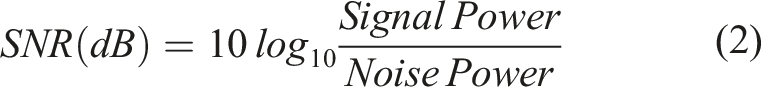
The convolutional layer is the main part of the CNN model. Each convolutional block contains learnable parameters such as weights (filters) and biases. Compared with the input, the width and the height of the filter are spatially smaller, but the depth is the same. For example, the RGB image has three layers, so, the convolutional layer should have 3 depths to analyze these three layers in the RGB image respectively. The feature maps from the previous layer are convolved with filters and formed the output through the activation function. The formula of the convolutional layer for a pixel is

C_{x y} = σ (\sum_{i = 1}^{h} \sum_{j = 1}^{w} \sum_{k = 1}^{d} f_{i j k} * X_{x + i, y + j - 1, k} + b)

(3)

where h and w are the sizes of the filter and d is the number of channels of the input, X is the input vector, b is the bias vector, σ is the activation function, and f is the weight matrix.

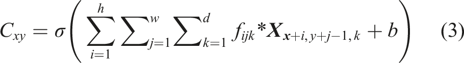
Figure 1 shows the convolution operation on a 4 × 4 matrix randomly selected. A 3 × 3 matrix is selected as the filter which is generated randomly at the initial state and updated from the model by a backward propagation algorithm.

Figure 1.

Process of the convolution layer.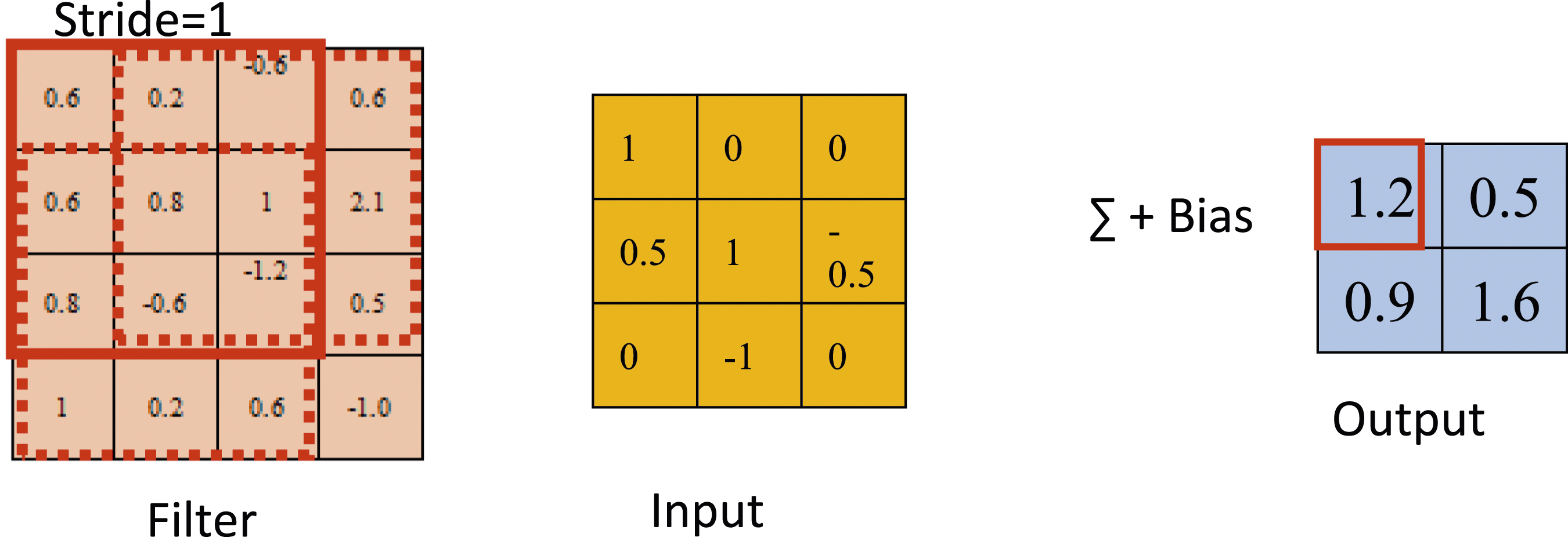

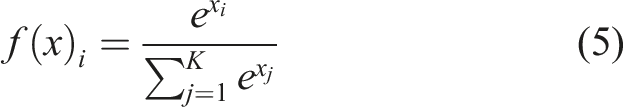
The stride is equal to one and four sub-arrays of the same size are generated by sliding along the width and height of the input matrix. Each sub-array is multiplied by the filter matrix. Then, the output value is obtained, which is the sum of the multiplied values and the bias. The size of the output is smaller than the previous layer because of the stride. After the convolution layer, a nonlinear activation function is followed, which is used for introducing non-linearity into the network and separating different classes. Two of the most common activation functions used in neural networks are rectifier linear unit (ReLU) and softmax. The function of ReLU and Softmax is expressed as follows:

f (x) = \max (0, x)

(4)

{f (x)}_{i} = \frac{e^{x_{i}}}{\sum_{j = 1}^{K} e^{x_{j}}}

(5)

Where f(x) is the parameter that could represent the probability for each group, and the notation x_i and x_j denote the current numerical values of the ith and jth neuron in the layer, K is the total number of neurons in the layer.

The pooling layer is used to reduce the spatial size of the feature maps to speed up the computation and increase the robustness of the feature detection. The most common ways are max pooling and average pooling. In max pooing, the maximum values in the filter area are chosen as outputs. For example, as shown in Figure 2, an input layer with the size of 4 × 4 is operated by a 2 × 2 max-pooling filter. The stride is designed as two which means the next filter should move by two positions to the right and down, which causes the dimension of the output to decline to 2 × 2, and the value in the cell is the maximum element in the response field. For the average pooling, average values would be calculated for the cell in the filter area.

Figure 2.

Process of the pooling layer.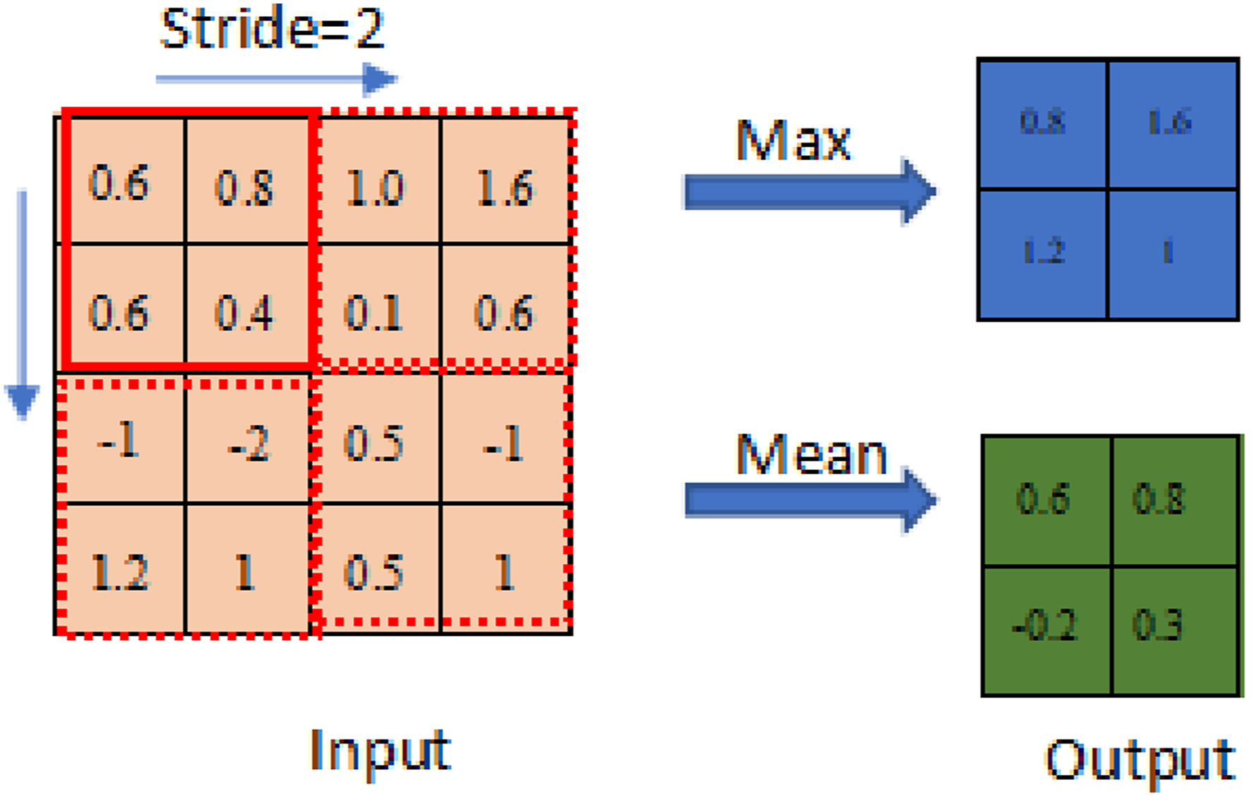

The fully connected layer is the last layer before the output layer of the whole network. In this layer, all the neurons are related to the features generated in the previous layer. Weights and biases in this layer convert the generated features into correspondent categories. The equation of the output y^l is shown:

y^{l} = σ (y^{l - 1} * w + b)

(6)

where σ is the activation function; w and b represent the weights and bias vectors in this layer respectively.

Different pretrained deep learning methods used

There are many pretrained deep learning methods that could be used. Several of these methods are summarized below, including (1) AlexNet, (2) GoogLeNet, (3) InceptionResNetv2, (4) ResNet50 and ResNet101, and (5) Vgg16 and Vgg19.

AlexNet is a very famous technique whose image classification performance is significantly accurate. AlexNet is a huge network with 60 million parameters and 650,000 neurons. The AlexNet has eight layers. Its first five layers are convolutional layers, and the last three layers are fully connected. Between these two groups of layers, there are some layers called polling and activation. Due to the low number of deep layers, this net can achieve a high accuracy in a short time.

Figure 3 presents the diagram of the AlexNet. The five convolutional layers and three connected layers are shown in this figure with different data sizes for each layer. The size of input images is 227 × 227 pixels. The number of categories in the final output is up to 1000.

Figure 3.

The diagram of AlexNet.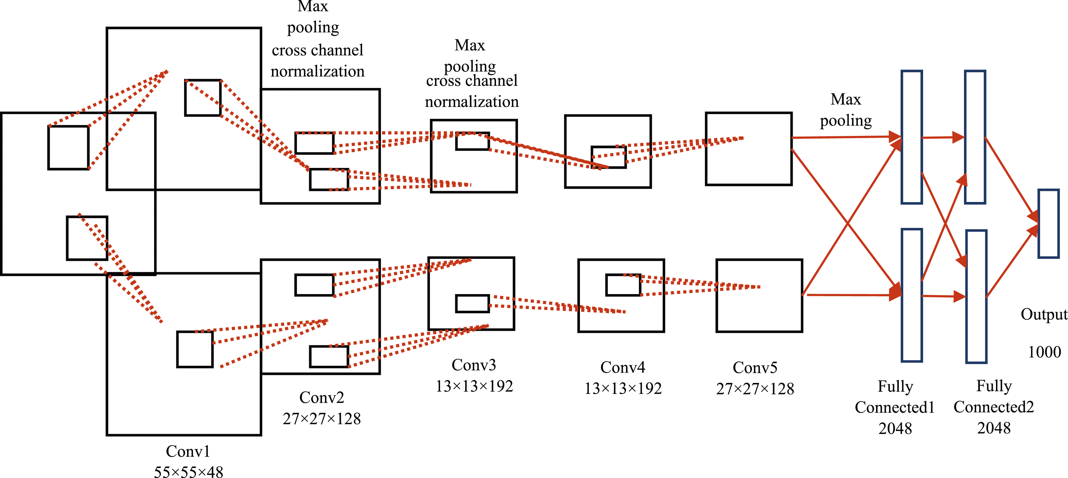

In the GoogLeNet model, the difference with AlexNet is that it has inception modules. In the inception module, 1 × 1, 3 × 3, 5 × 5 convolution layers and 3 × 3 max-pooling layers are performed and the output of these layers is stacked together to generate the final output. Thus, the GoogLeNet could handle objects at multiple scales better.

The InceptionResNetv2 is a kind of convolutional neural network which has 164 layers and could classify images up to 1000 categories. This model takes a long time to be trained as it contains 164 deep layers.

The ResNet-50 model consists of five stages each with a convolution and identity block. Each convolution block has three convolution layers, and each identity block also has three convolution layers as shown in Figure 4. The ResNet-50 model has over 23 million trainable parameters. The difference between ResNet50 and ResNet101 is that the ResNet-101 model has 101 layers.

Figure 4.

The architecture of the ResNet50 algorithm.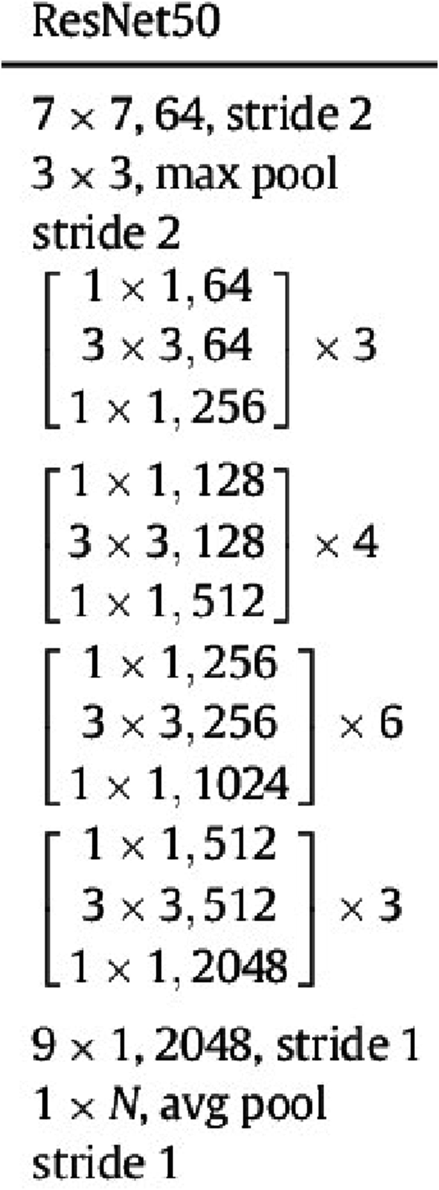

VGG-16 is a convolutional neural network that is 16 layers deep. The model loads a set of weights pre-trained on ImageNet. The model achieves 92.7% test accuracy in ImageNet, which is a dataset of over 14 million images belonging to 1000 classes. The default input size for the VGG16 model is 224 × 224 pixels with three channels for RGB images.

The concept of the VGG19 model is the same as the VGG16 model except that it supports 19 layers. The “16” and “19” stand for the number of weight layers in the model (convolutional layers), which means that VGG19 has three more convolutional layers than VGG16 does.

Data collection through ABAQUS modeling

Figure 5(a) shows a schematic diagram of the beam modeled using ABAQUS. There are 10 segments (S1 to S10) and 10 measurement locations (MP1 to MP10). For each case, different segments would be damaged by reducing their Elastic Modulus by 30%. Then a concentrated force (CF) is applied to the free end of the cantilever beam. Then the CF is released to let the cantilever beam perform free vibration. Thus, the vibrations at each measured point can be obtained. These vibrations need to be labeled and included in the training set of the CNN model. Figure 5(b) shows the beam model in ABAQUS, in which one end is fixed, and the other end is free.

Figure 5.

(a) The beam model in ABAQUS; (b) The applied load, boundary condition, and the measurement points in the beam model.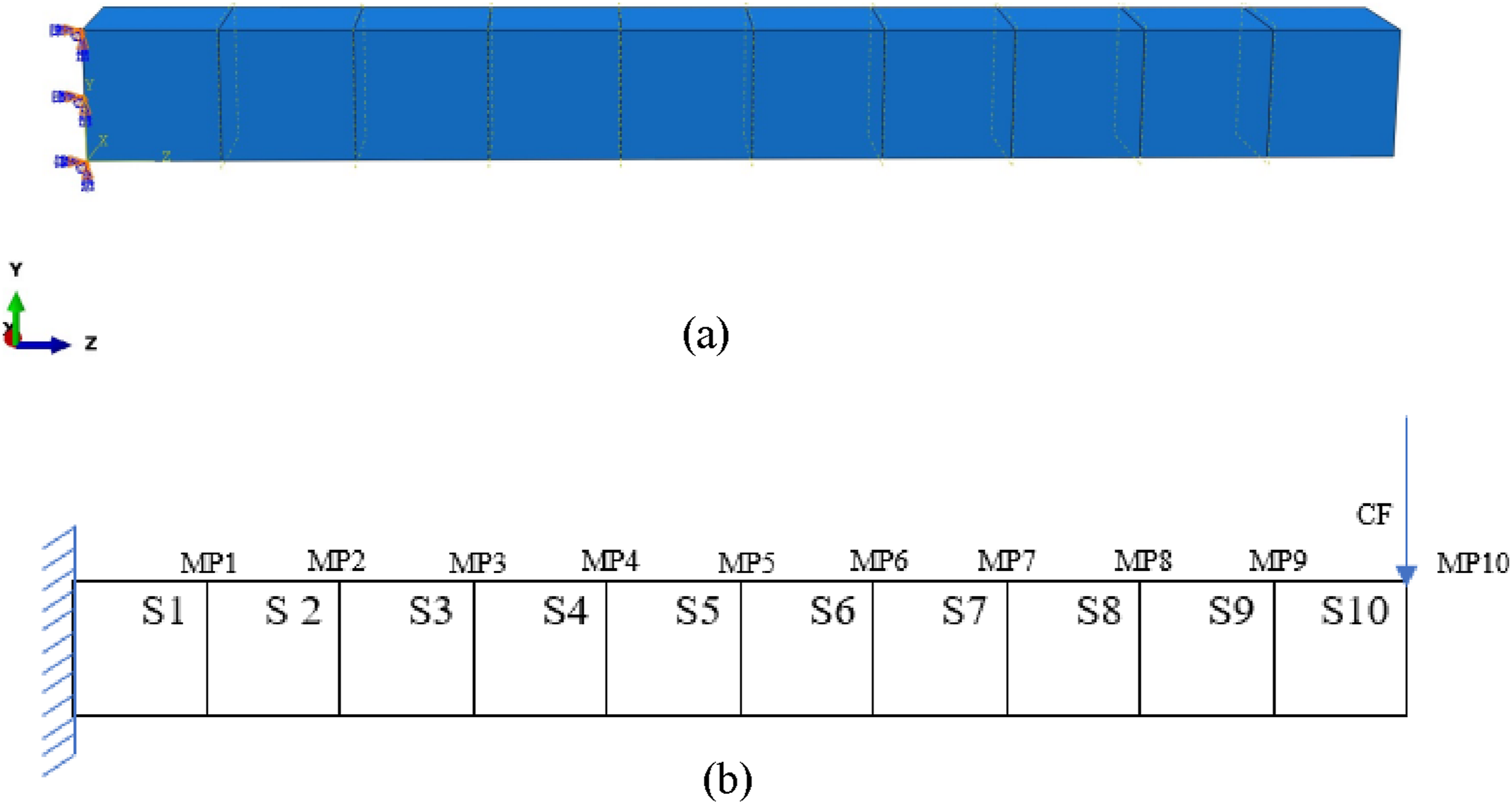

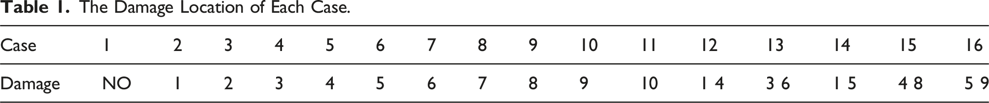
Table 1 shows the different damage locations of each case. There are 10 cases with one damage location (2 to 11), one healthy beam (1), and 5 cases (12 to 16) with two damage locations. For example, the No.14 case represents a case with damages at element one and element 5.

Table 1.

The Damage Location of Each Case.

Case	1	2	3	4	5	6	7	8	9	10	11	12	13	14	15	16
Damage	NO	1	2	3	4	5	6	7	8	9	10	1 4	3 6	1 5	4 8	5 9

As shown in Figure 6, another modeling of a cantilever beam in ABAQUS is conducted. The beam is divided into 256 elements and there are 15 cases with different damage locations. There is one case with a health beam, seven cases with one damage location, four cases with two damage locations, two cases with three damage locations, and one case with four damage locations. The damage of the element was performed by reducing the Young’s modulus to 70%. Vibrations of the beam were triggered by the release of a concentrated force at the free end of the beam. The 16 measured points are shown as red points in Figure 6(15). Gaussian noise was used to enlarge the training dataset and finally, there are 7500 samples in total for the deep learning models.

Figure 6.

(0)-(14): All cases in ABAQUS modeling with different damages; (15) 16 measurement points.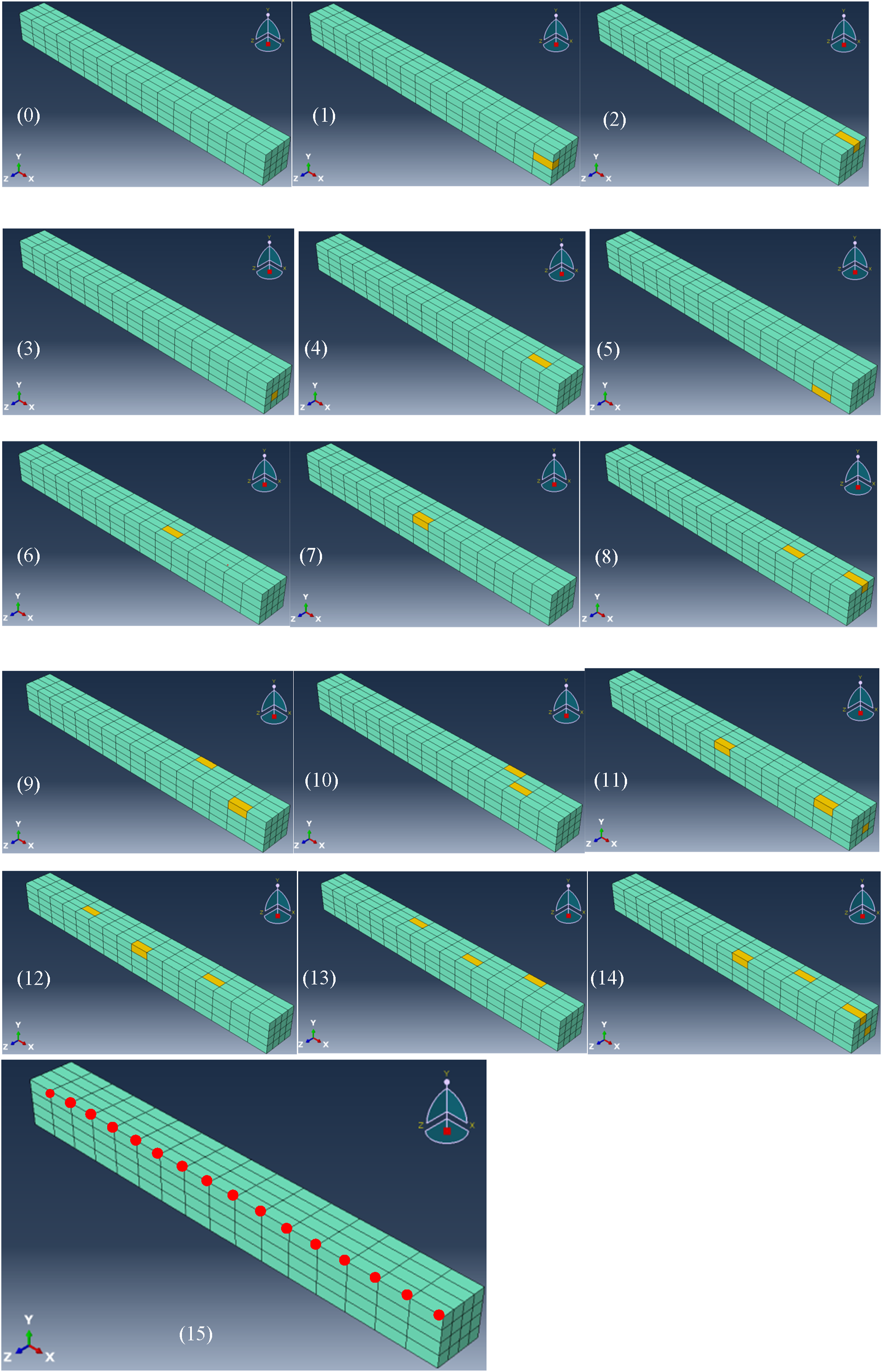

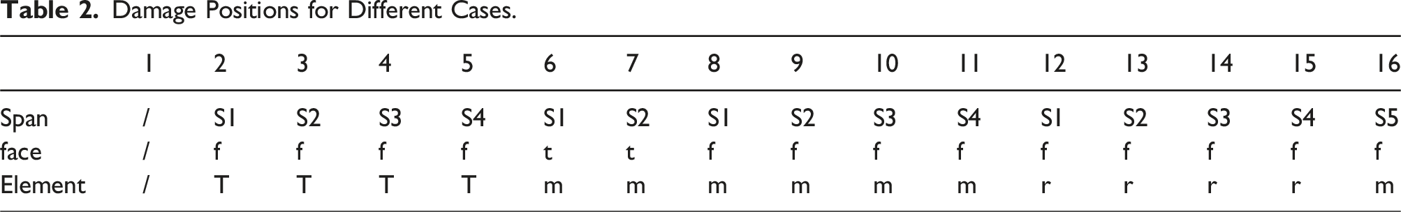
Figure 7 shows a truss model in ABAQUS. The truss in this study has eight spans and there are 10 measured points on the truss. Table 2 shows the damage locations of different cases and there are 16 cases in total. f represents the front face and t represents the top face of the truss. t, m, and r in the element category represent the top element, the middle element, and the right element respectively. There are five spans as shown in Figure 9. For example, case number 8, the sloping rod on the front face is damaged by reducing 30% of its elastic modulus. No. 5 case represents the damage on the top element of the front face at the fourth span of the truss.

Figure 7.

Modeling of the truss in ABAQUS.

Table 2.

Damage Positions for Different Cases.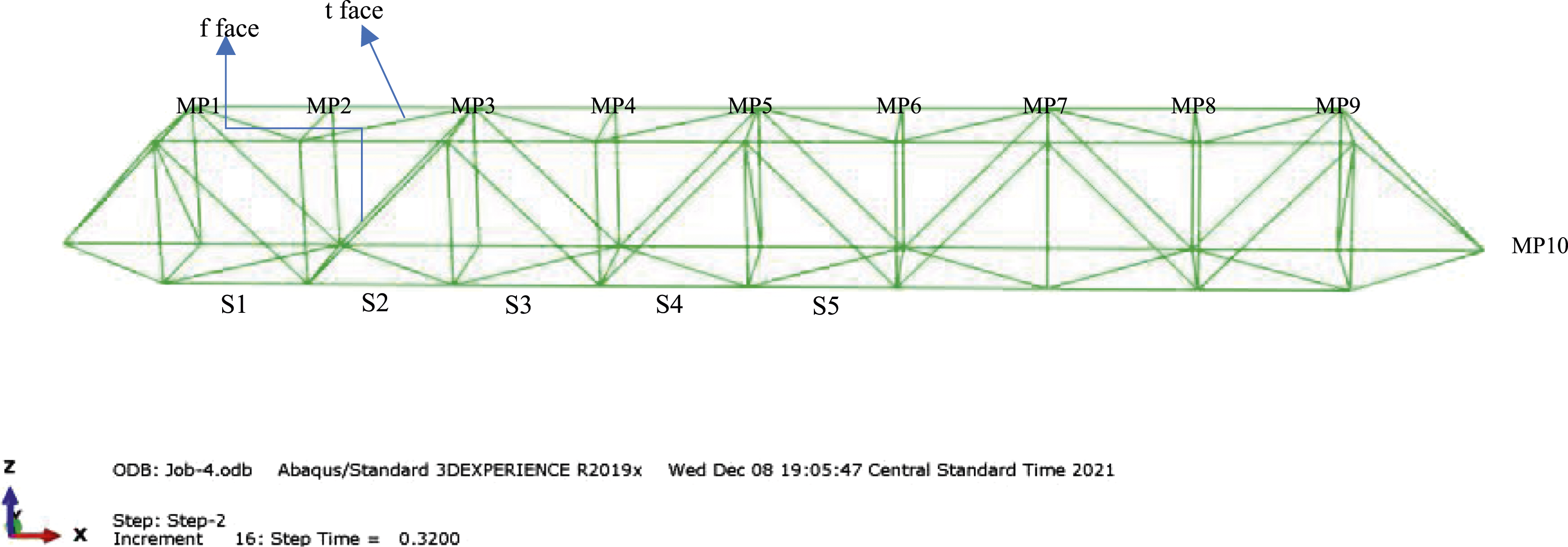

	1	2	3	4	5	6	7	8	9	10	11	12	13	14	15	16
Span	/	S1	S2	S3	S4	S1	S2	S1	S2	S3	S4	S1	S2	S3	S4	S5
face	/	f	f	f	f	t	t	f	f	f	f	f	f	f	f	f
Element	/	T	T	T	T	m	m	m	m	m	m	r	r	r	r	m

Results of model training, validation, and prediction

The above-described process has resulted in satisfactory outputs using the beam and truss cases. For beam 1, the changes are obvious after applying noise, which could enlarge the data set tremendously, as shown in Figure 8 by comparing (a) the original vibration data with (b) the vibration data with inclusion of the noise.

Figure 8.

(a) The original vibration data; (b) The vibration data after applying noise.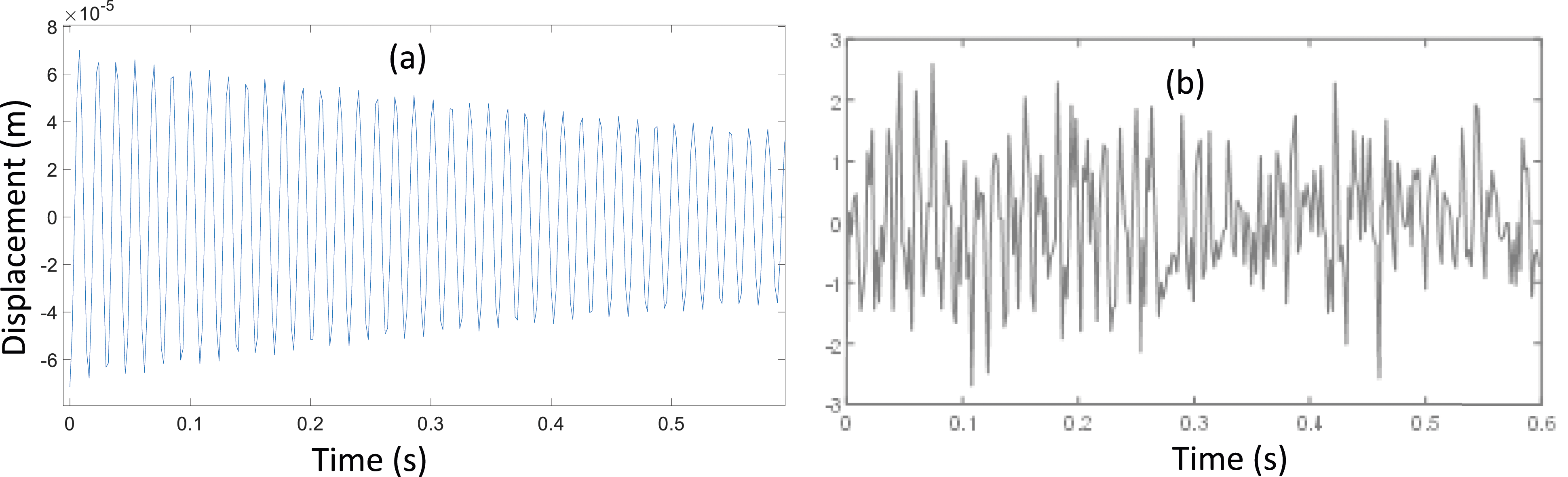

As shown in Figure 9, the accuracy is 73.88% for the case that the SNR is 90 dB. Moreover, the main error exists at point 8, point 9 and point 10, which is partially because the damage at a location far from the fixed end will have a small influence on the dynamic characters of a cantilever beam. And the 2-damage case would be affected by the cases which have at least one same damage location, such as Case 4 and Case 48.

Figure 9.

The training results when the noise is 90 dB. (a) the training error and validation error; (b) Prediction results.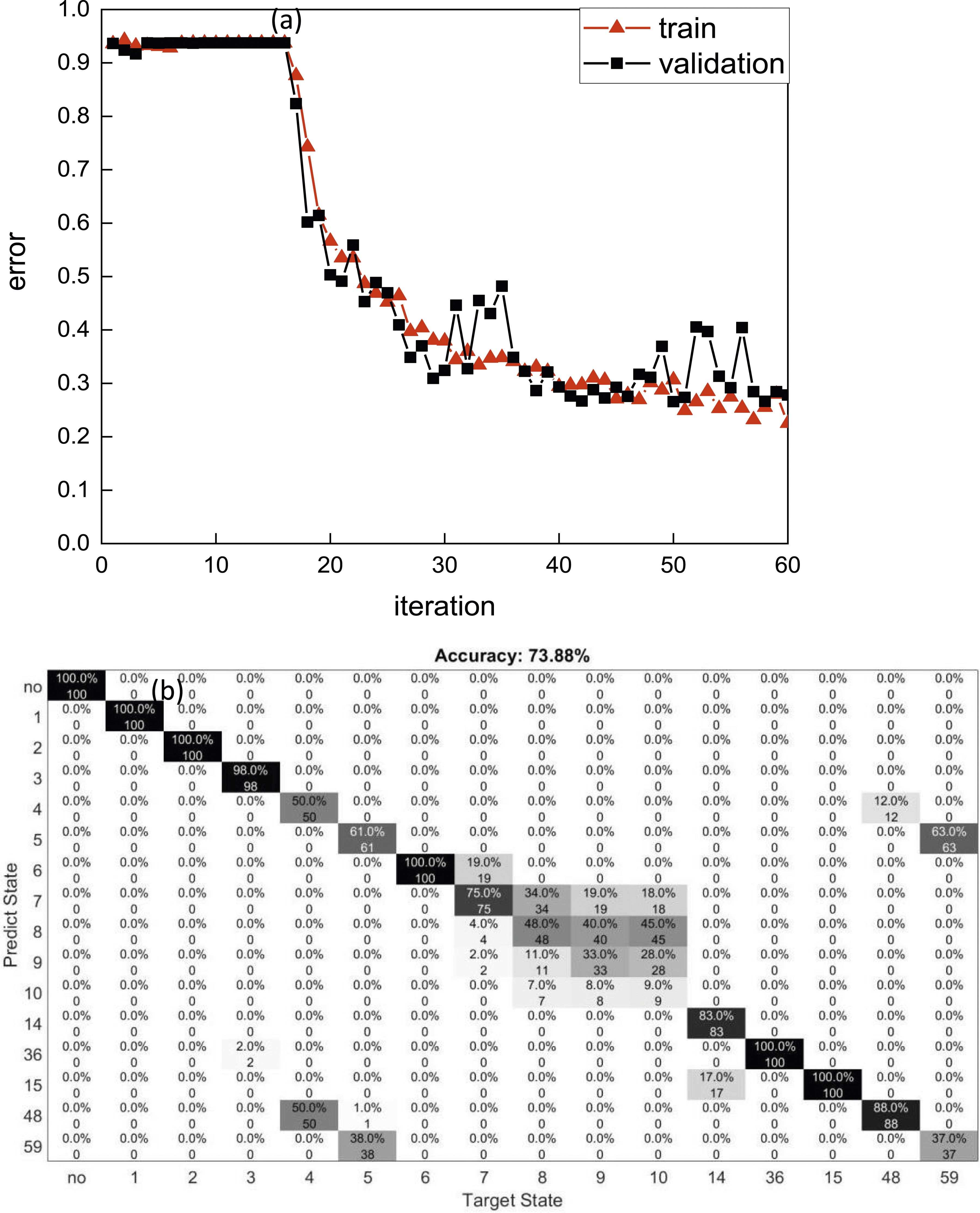

All the other SNR ratios were also simulated, and their prediction accuracies are included in Table 3 for comparison.

Table 3.

The Accuracy of Different Cases With Different SNRs

Noise level	90 (%)	100 (%)	110 (%)	120 (%)	130 (%)
Accuracy	73.88	90.44	93.63	94.13	99

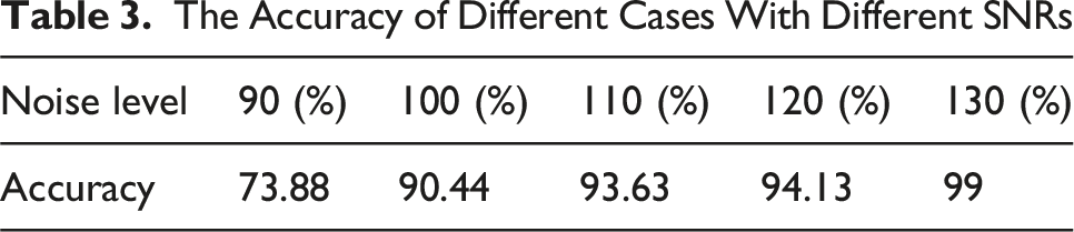
For beam 2, similar results can be observed in Figures 10 and 11. When the SNR is below 90 dB, the accuracies are between 80% to 90%. When the SNR is from 90 dB to 120 dB, the accuracy is near 100%. For cases with SNR higher than 120 dB, the accuracy is 100%. Cases with one damaged location have more errors. However, cases with more than one damaged location have higher accuracy.

Figure 10.

Vibration curves after applying different noises comparing with healthy vibrations. (a) 80 dB; (b) 85 dB; (c) 100 dB; (d) no noise.

Figure 11.

Testing results of the training process with noise at (a) 80 dB; (b) 85 dB; (c) 90 dB; (d) 95 dB; (e) 100 dB; (f) 110 dB; (g) 120 dB; (h) 130 dB.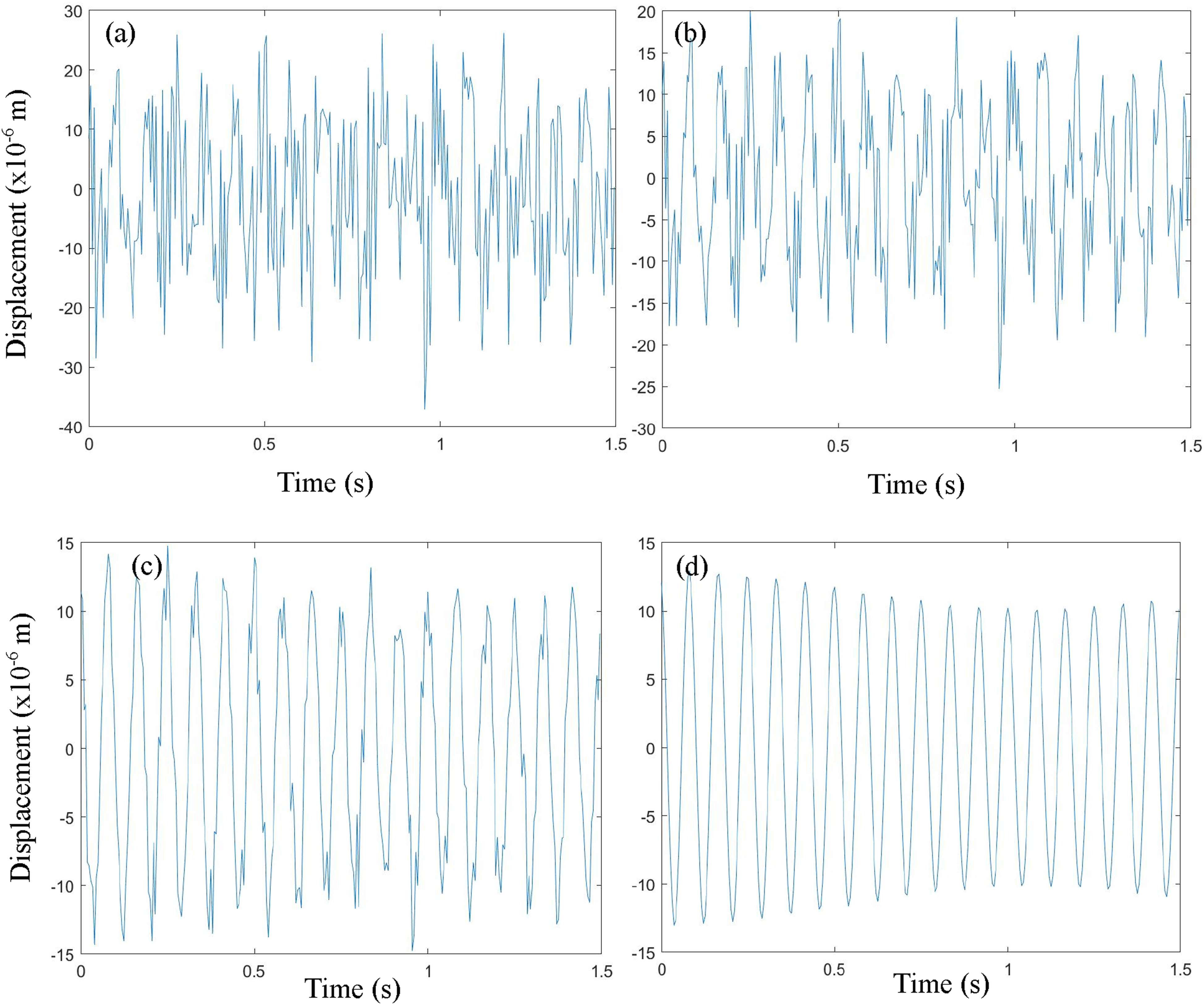

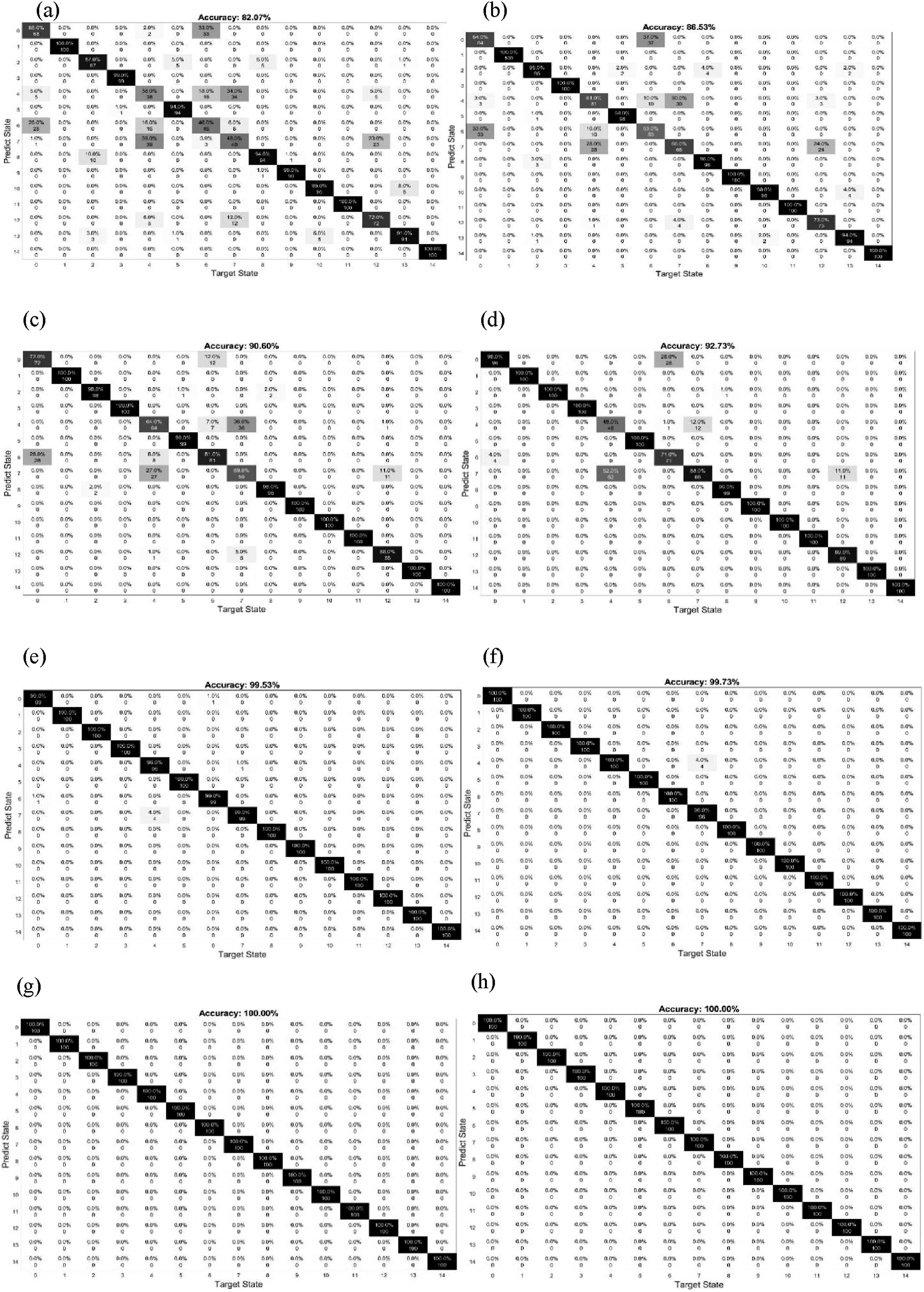
Figure 12 shows the training processes with different SNR levels. Smaller SNR would need more iterations to achieve stability for the training curves. As the SNR becomes smaller, the accuracy would be lower and there are bigger gaps between training loss and validation loss.

Figure 12.

Training processes with noise at (a) 80 dB; (b) 85 dB; (c) 90 dB; (d) 95 dB; (e) 100 dB; (f) 110 dB; (g) 120 dB; (h) 130 dB.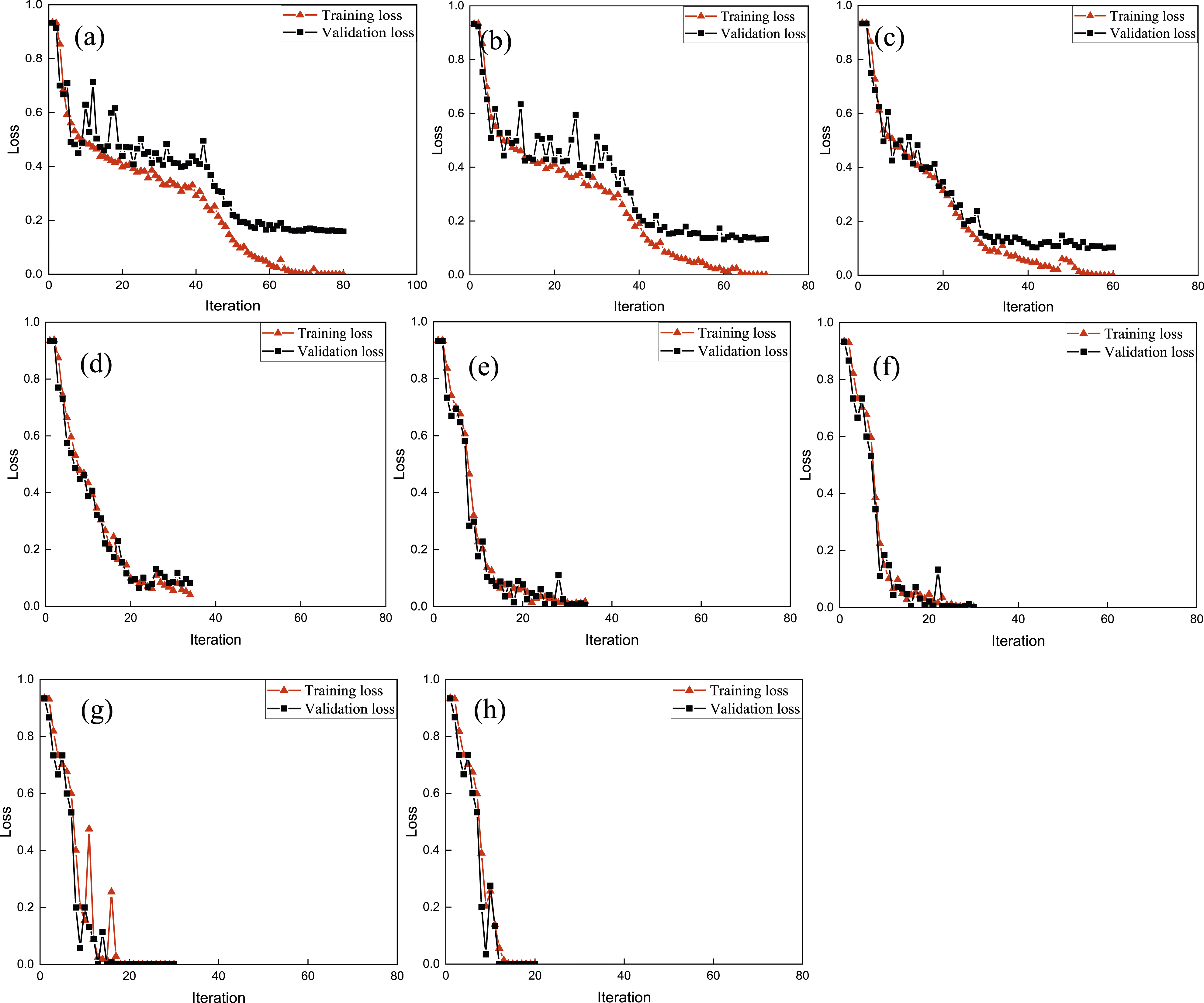

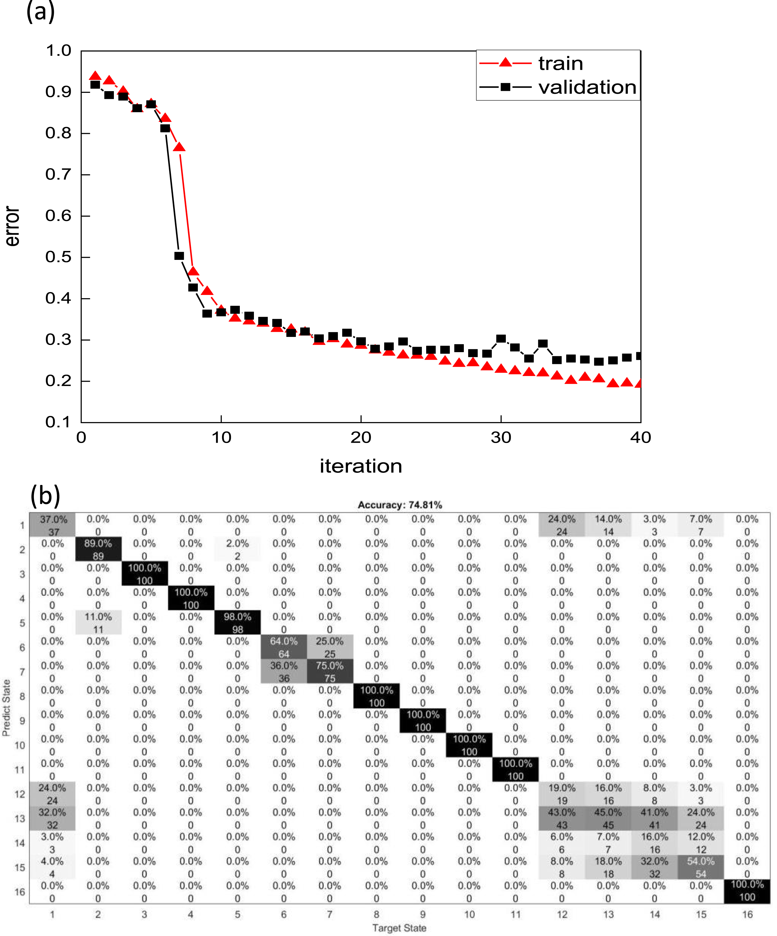
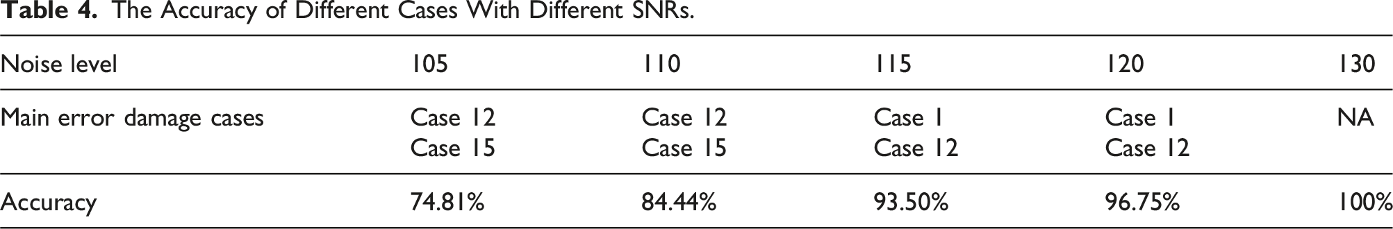
However, for the truss case, as shown in Figure 13, the changes are not significant after applying noise. As shown in Figure 14, the overall accuracy is 74.81% for the case when the SNR is 105 dB. Moreover, the main error exists between Case 12 and Case 15 whose damage is on the vertical elements in the front face. Because those damages cause a small change in the stiffness and dynamic characteristics of the truss, their effects on the vibration are similar. All the other SNR ratios were also simulated, and their prediction accuracies and the main error damage cases are listed in Table 4 for comparison.

Figure 13.

(a) The original vibration data; (b) The vibration data after applying noise.

Figure 14.

The training results when the noise is 105 dB. (a) the training error and validation error; (b) Prediction results.

Table 4.

The Accuracy of Different Cases With Different SNRs.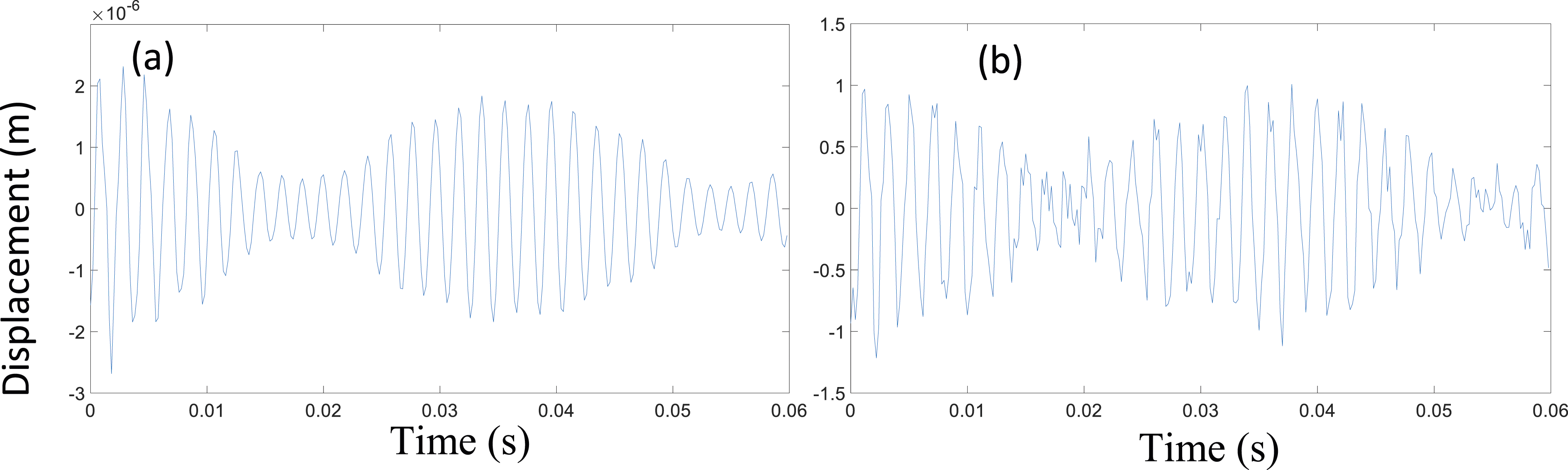

Noise level	105	110	115	120	130
Main error damage cases	Case 12	Case 12	Case 1	Case 1	NA
Main error damage cases	Case 15	Case 15	Case 12	Case 12	NA
Accuracy	74.81%	84.44%	93.50%	96.75%	100%

Results of crack detection using deep learning-based image classification

Figure 15 shows two groups of labeled images that are with-crack images and no-crack images. There are 20,000 with-crack images and 20,000 no-crack images for training the proposed pretrained deep learning method. Some with-crack images of different widths, different lengths, different directions, and different image brightness are collected for training the model. Figure 16 shows the training process of the proposed method. The method is very fast and effective because, after only several epochs, both testing accuracy and validation accuracy are close to 100%. Some sharp changes in the training accuracy were found due to overfitting. The features of cracking in images are simple and do not need too many training iterations to find them. The CNN model is prone to overfitting because of the millions or billions of parameters it encloses.

Figure 15.

Samples of training images.

Figure 16.

The training accuracy and validation accuracy using AlexNet.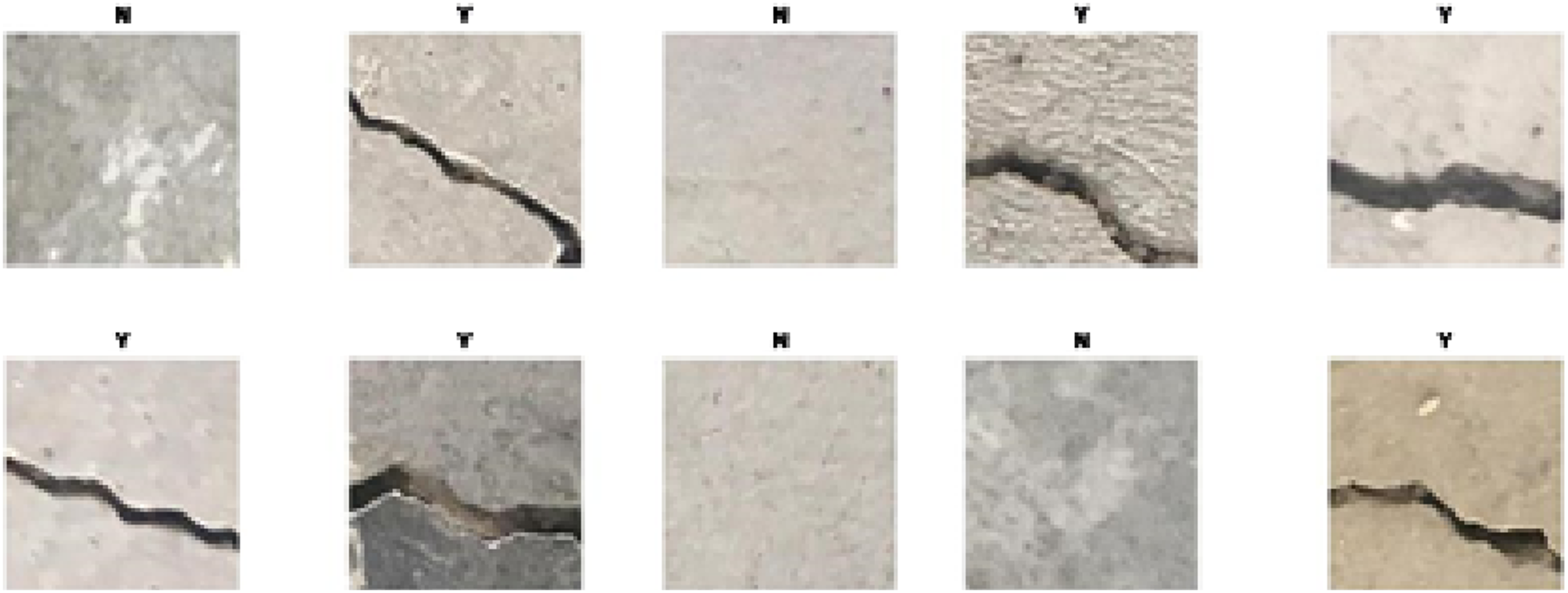

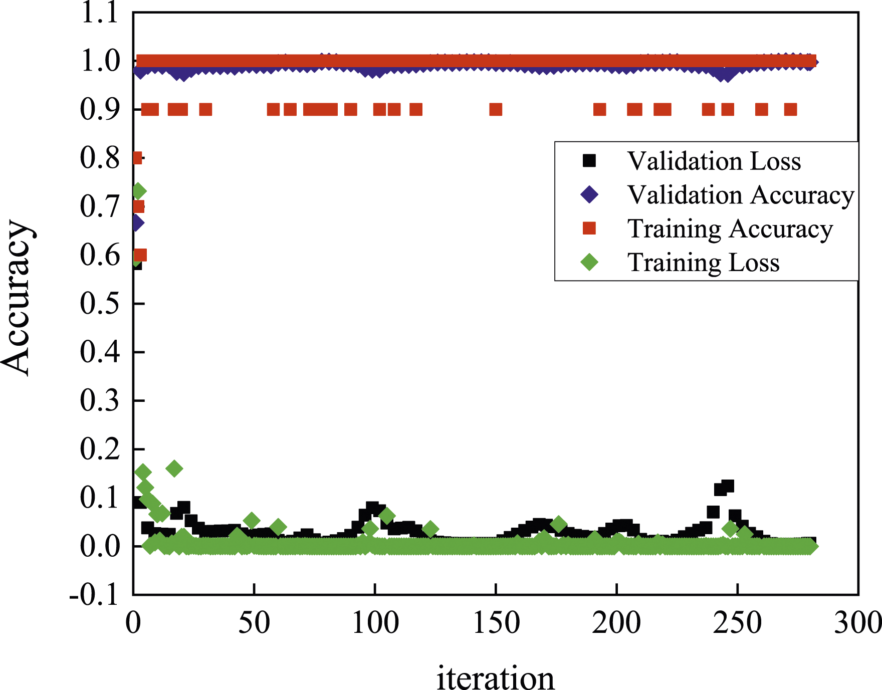
Figure 17 shows the training process with its training and validation accuracy using VGG16. The training and validation accuracy reaches nearly 100% after only several iterations. The training loss and validation loss decrease quickly to zero after 50 iterations. There are some peaks for all these four curves, which are due to the overfitting errors. Moreover, after these peaks, these curves return to stability quickly. Figure 18(a) shows the with-crack image captured in the field and Figure 18(b) shows the results of all proposed methods. Moreover, each segment of the crack in the with-crack image was detected successfully.

Figure 17.

The training accuracy and validation accuracy using VGG16.

Figure 18.

The testing results using an image captured in the field: (a) the captured image; (b) the output image using the proposed method.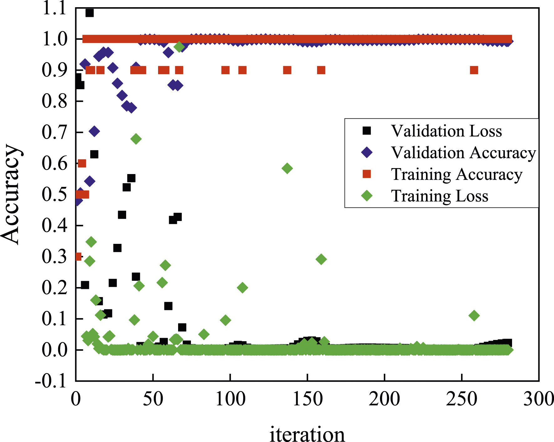

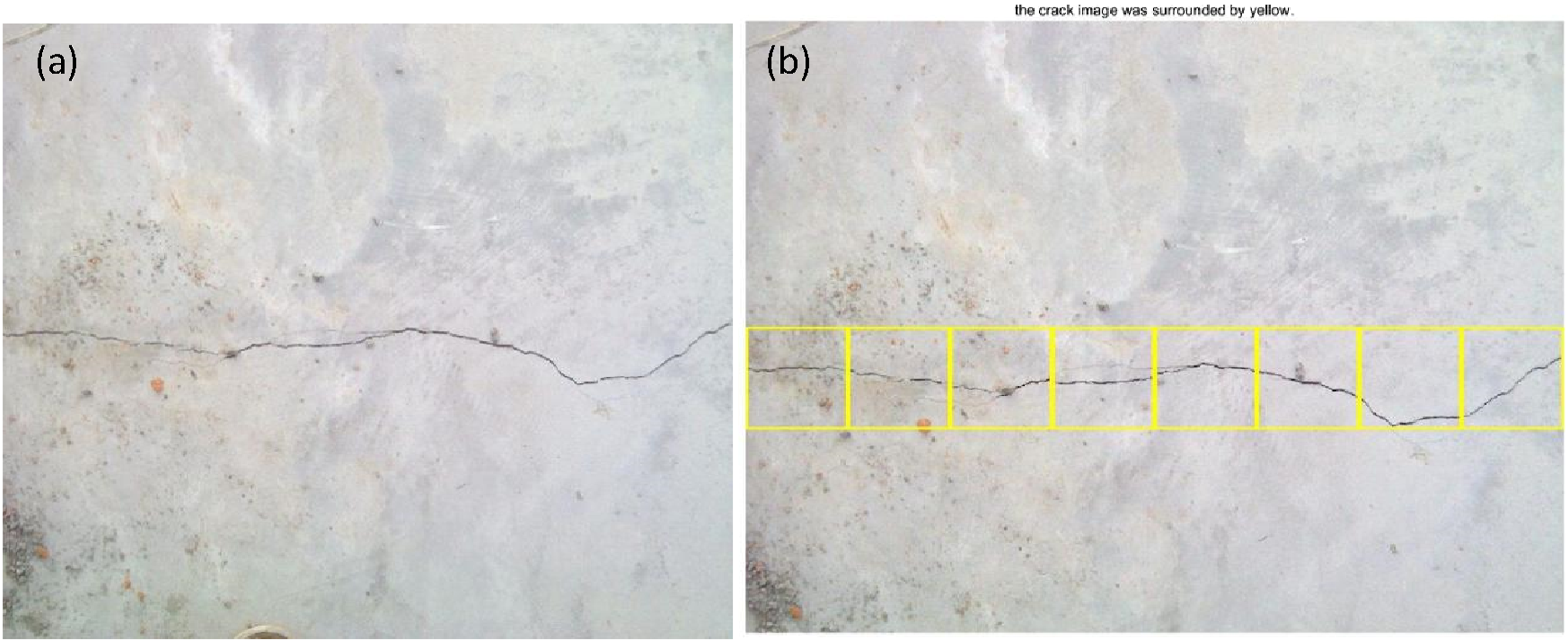
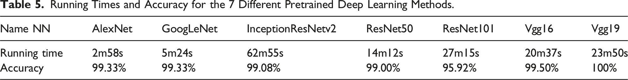
Figure 19 shows the testing results of the proposed method using images in the same dataset with the training data. ‘N’ represents the label of no-crack images and ‘Y’ represents the label of with-crack images. The accuracy of the testing results of 20 images is 100%. Table 5 shows the running time and accuracy for each deep learning method trained by the crack dataset. The AlexNet model has the smallest running time (2m58s) and the InceptionResNetv2 model has the most running time (62m55s). The ResNet101, Vgg16, and Vgg19 models have similar running times which are about 20 min. The GoogleNet and ResNet50 model have 5m24s and 14m15s on the running time respectively. The accuracy of the RetNet101 model is less than 99%, and the accuracies of the rest of those methods are more than 99%.

Figure 19.

The testing results with the images in the same dataset of the training data.

Table 5.

Running Times and Accuracy for the 7 Different Pretrained Deep Learning Methods.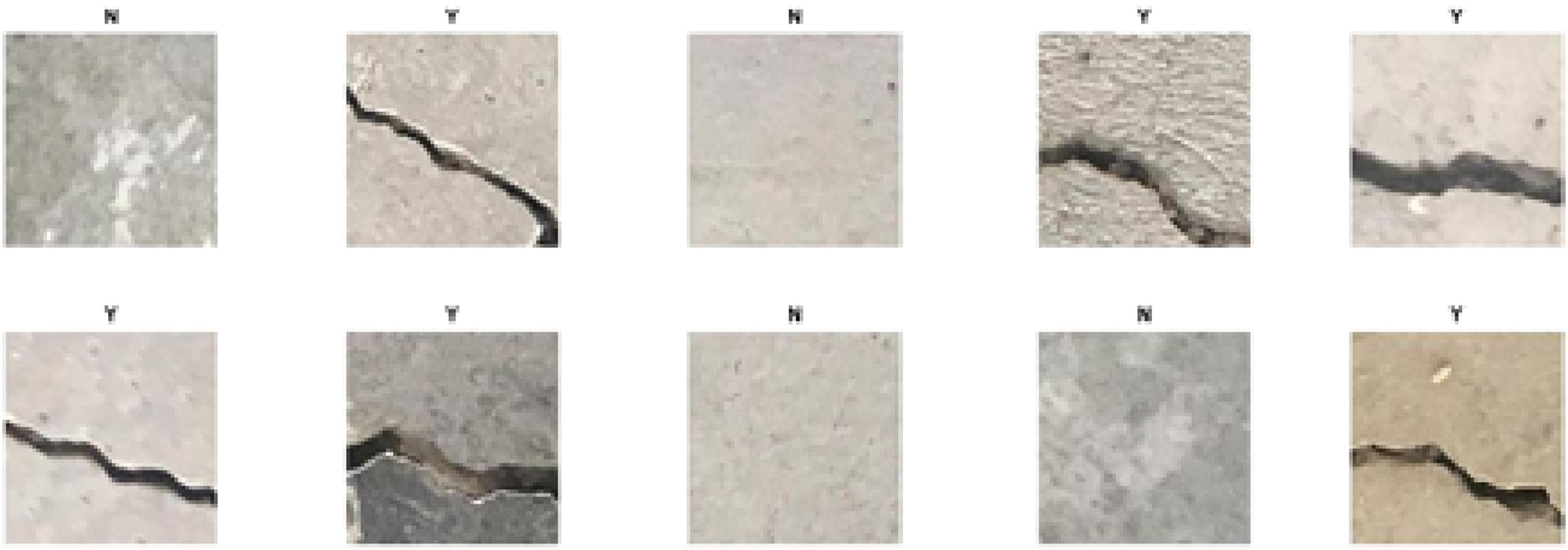

Name NN	AlexNet	GoogLeNet	InceptionResNetv2	ResNet50	ResNet101	Vgg16	Vgg19
Running time	2m58s	5m24s	62m55s	14m12s	27m15s	20m37s	23m50s
Accuracy	99.33%	99.33%	99.08%	99.00%	95.92%	99.50%	100%

Structural evaluation using a novel deep-learning-based method with both defect image and vibration data

As shown in Figure 20, images of defects at important positions of a structure are captured by cameras or UAVs. The vibration data of the structure is obtained by displacement or accelerometer sensors. These one-dimension vibrations are converted into two-dimension images. These two groups of images are then combined to provide input data for the suggested deep-learning model.

Figure 20.

The process of the proposed damage evaluation method using images of vibration and raw images of defects.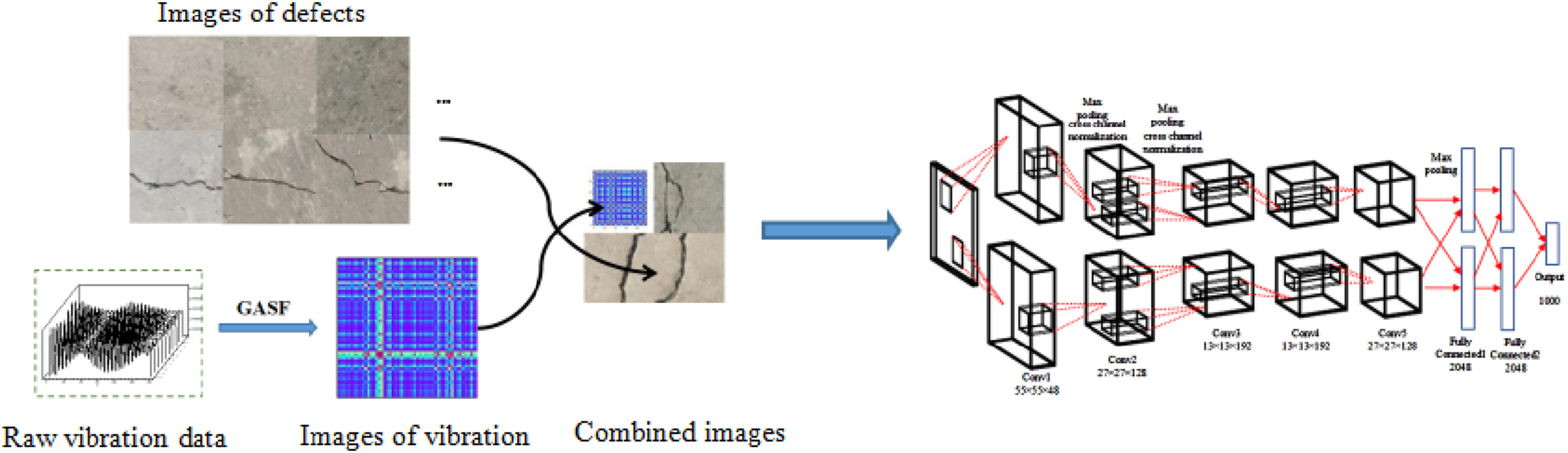

Gramian angular field

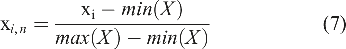
In the field of time series data, the GAF algorithm was created to encode 1D time series into 2D images without losing any features (Tran et al., 2013). GAF can be completed through two different algorithms: gramian angular sum field (GASF) and gramian angular difference field (GADF). The vibration data is X = {x₁, x₂, …, x_i, …, x_n}, where n is the total number of displacement points and x_i is the value of the displacement. The second step is to normalize the spectral data and scale it to the range of [0, 1], and record it as x_i,n.

x_{i, n} = \frac{x_{i} - \min (X)}{\max (X) - \min (X)}

(7)

Next, the 1D spectral sequence in the Cartesian coordinate system is transformed into a polar coordinate system using the formula:

φ = \arccos (x_{i, n})

(8)

The Gramian matrix retains time dependent. Since time increases as the position moves from the upper left corner to the lower right corner, the time dimension is encoded into the geometry of the matrix. It can be seen from equation (8) that the value range of the converted angle ϕ is [0, π], and the cosine value decreases monotonically within this range. With the increase of wavelength, x_i in each Cartesian coordinate system only corresponds to the angle value in the polar coordinate system, time t corresponds to the radius in the polar coordinate system, and the corresponding bending occurs between different angle points on the polar coordinate circle. By calculating the cosine value of the sum of angles between different points, we can get the following formula for the calculation of the gramian angular summation field (GASF):

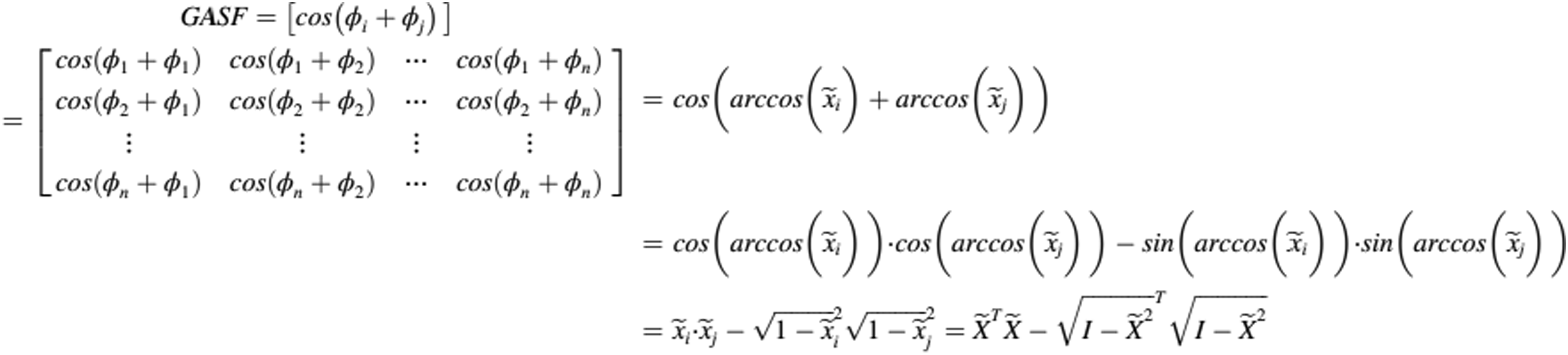where, I is the unit vector. ${\tilde{X}}_{i}$ is the normalized vibration data. φ is the angle of the point.

Figure 21(a) shows an example using the vibration data obtained from the ABAQUS model of the steel truss. The vibration is converted into images using the proposed GASF and there are many obvious features in the image, such as the highlighted points and lines in Figure 21(b).

Figure 21.

Example of GASF. (a) raw vibration obtained in ABAQUS model; (b) Images obtained by GASF.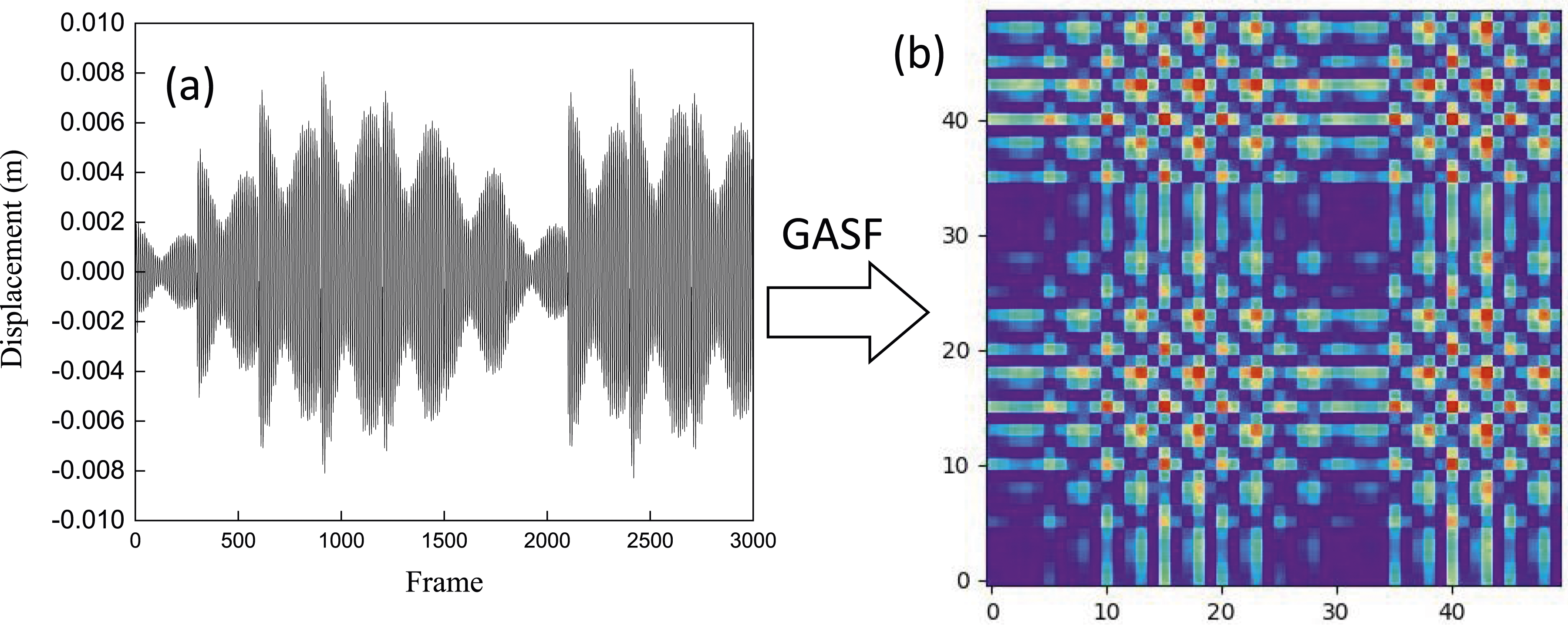

Flowchart of the proposed method

A flowchart of the proposed method is shown in Figure 22. This flow chart demonstrates the proposed method where the data is collected first by different sensors and cameras. Then the vibration data are converted to 2D images using the Gramian Angular Summation Field method. After that, image processing (resize) is deployed on all images. Subsequently, images of vibration data and optical structural defect images are combined. Finally, the pretrained deep learning model is fed with the fused images to predict abnormal defects at the location.

Figure 22.

Flow chart of the proposed method.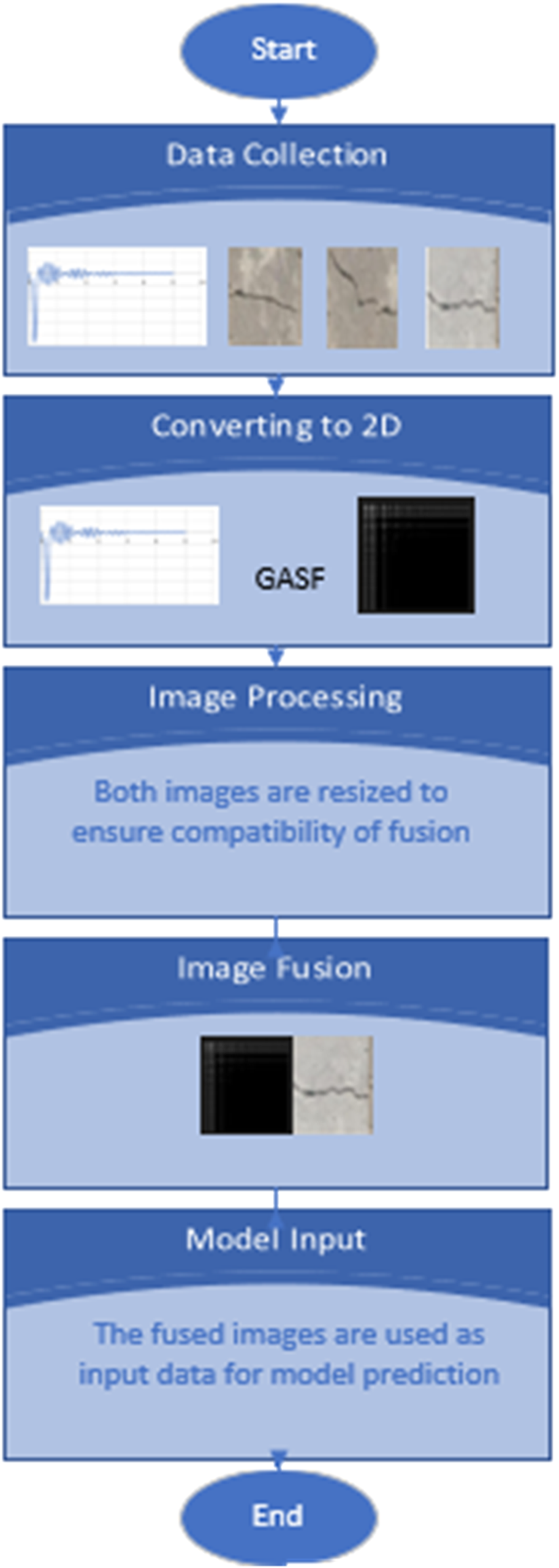

Results of the proposed method

To verify this method, the truss model in Figure 7 was adopted. The damage is simulated by reducing 30% of the Elastic modulus of the damaged truss member. A dynamic load is applied at the mid-point of the truss, and dynamic displacement data is collected at the specified measurement point. Figure 23 shows the dynamic displacement of a damage case on the MP2 location.

Figure 23.

Dynamic displacement at MP2 obtained from ABAQUS.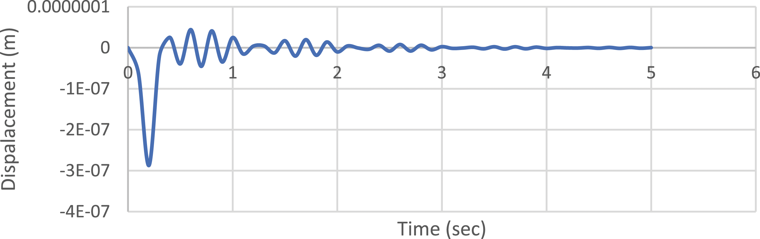

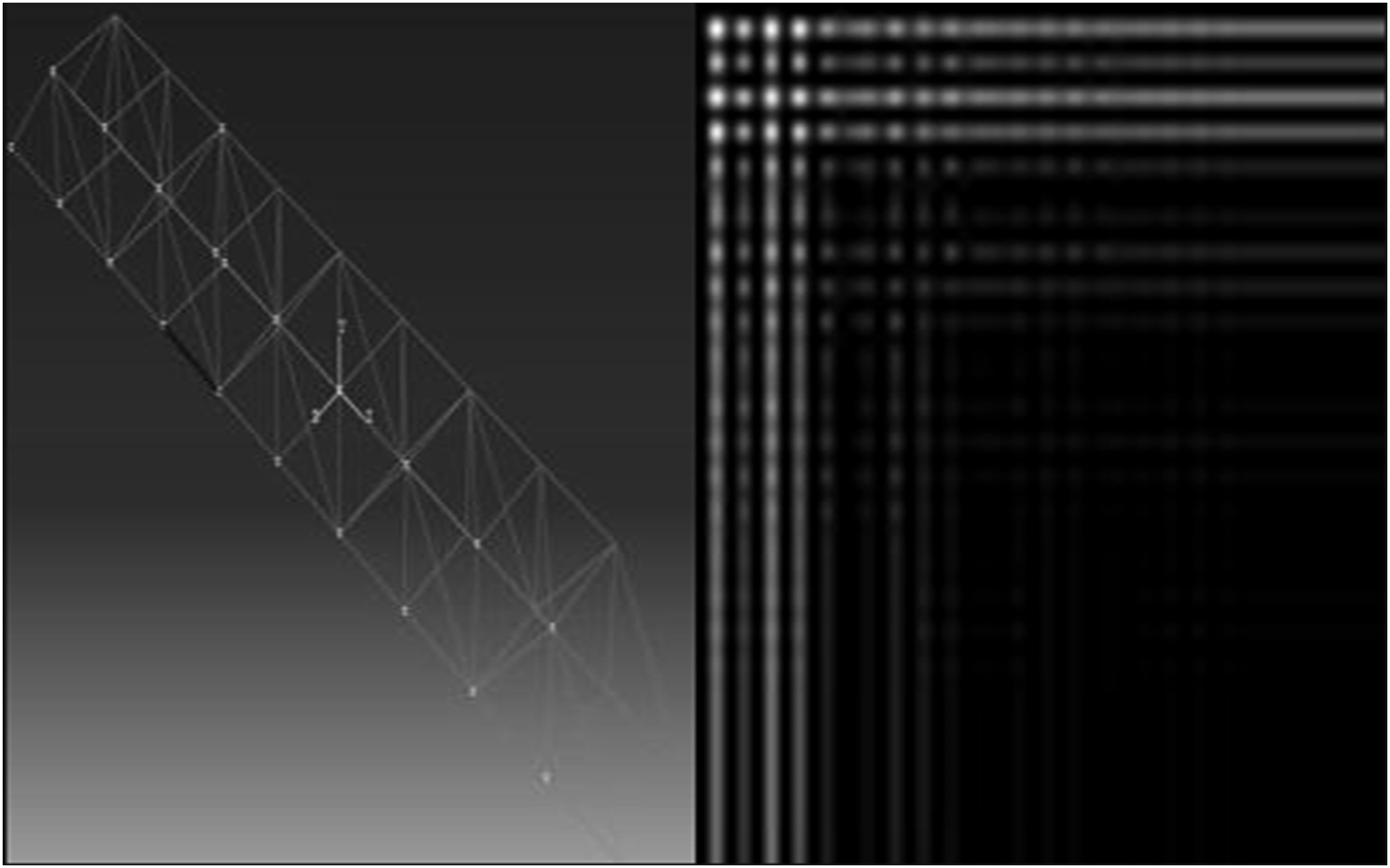
These displacements were converted from 1D to 2D using the GASF method. Figure 24 shows the GASF image of the dynamic displacement at MP2 for a damaged case. These images were then combined with the corresponding damaged optical photo, which is highlighted with the black color for the damaged element, to obtain full mapping of the damage as shown in Figure 25.

Figure 24.

Converted GASF dynamic displacement at MP2.

Figure 25.

Combined image of the optical truss damage photo and the converted GASF dynamics displacement.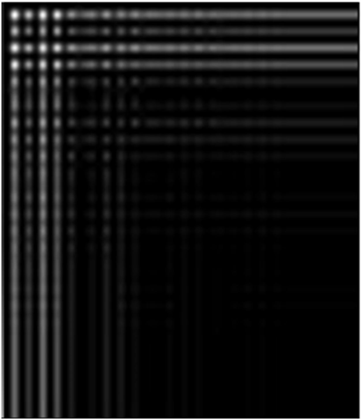

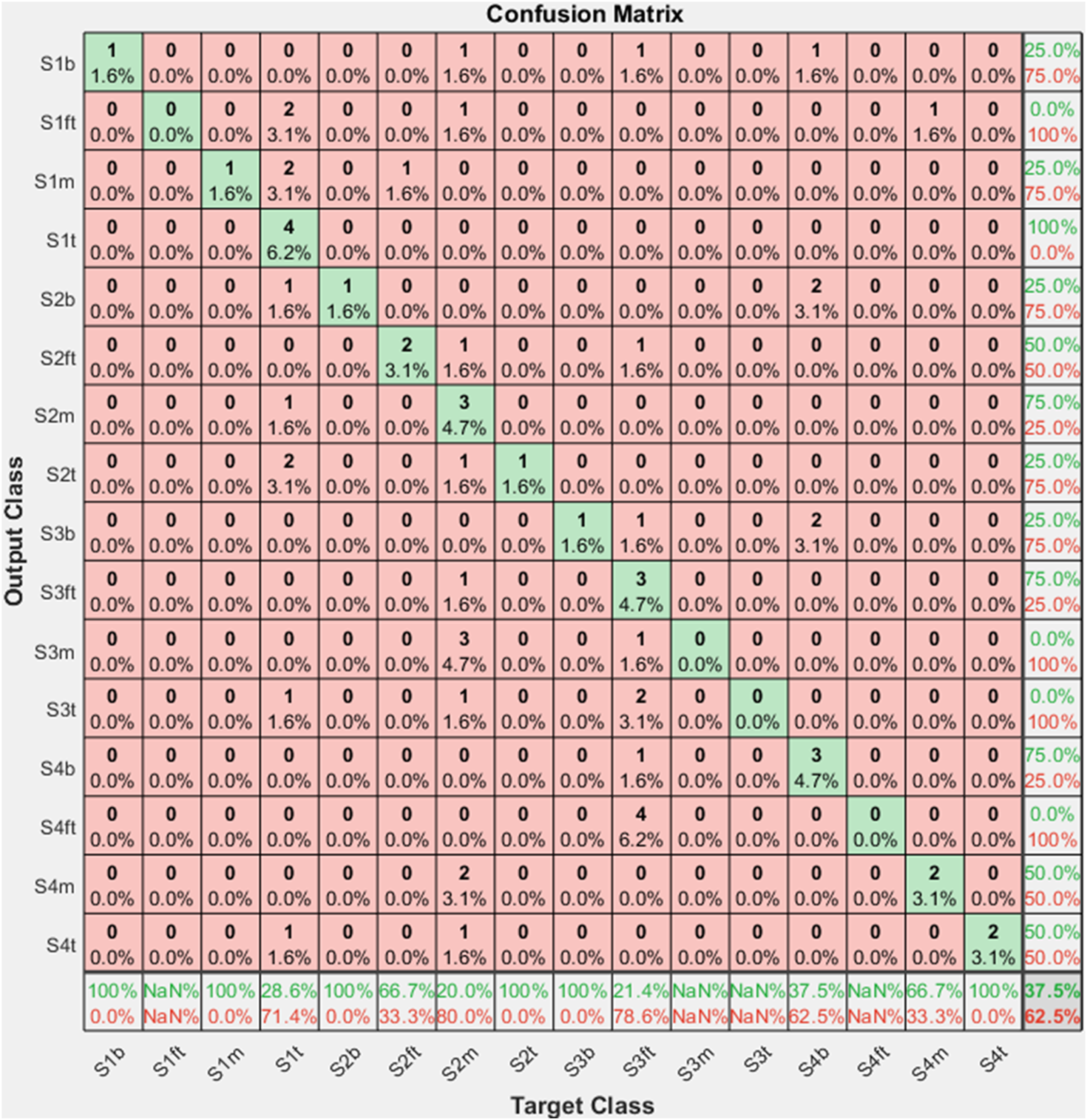
For validation purposes, the GoogleNet model was adopted in damage detection with various damage scenarios. When trained exclusively on optical damage photos, the GoogleNet model achieves an accuracy of 37.5% as shown in Figures 26 and 27. It illustrates the inherent challenges in accurately discerning structural damages based solely on visual images, especially for the case with blurred photos.

Figure 26.

The training results using optical images of damaged trusses as input.

Figure 27.

The confusion matrix using optical images of damaged trusses as input.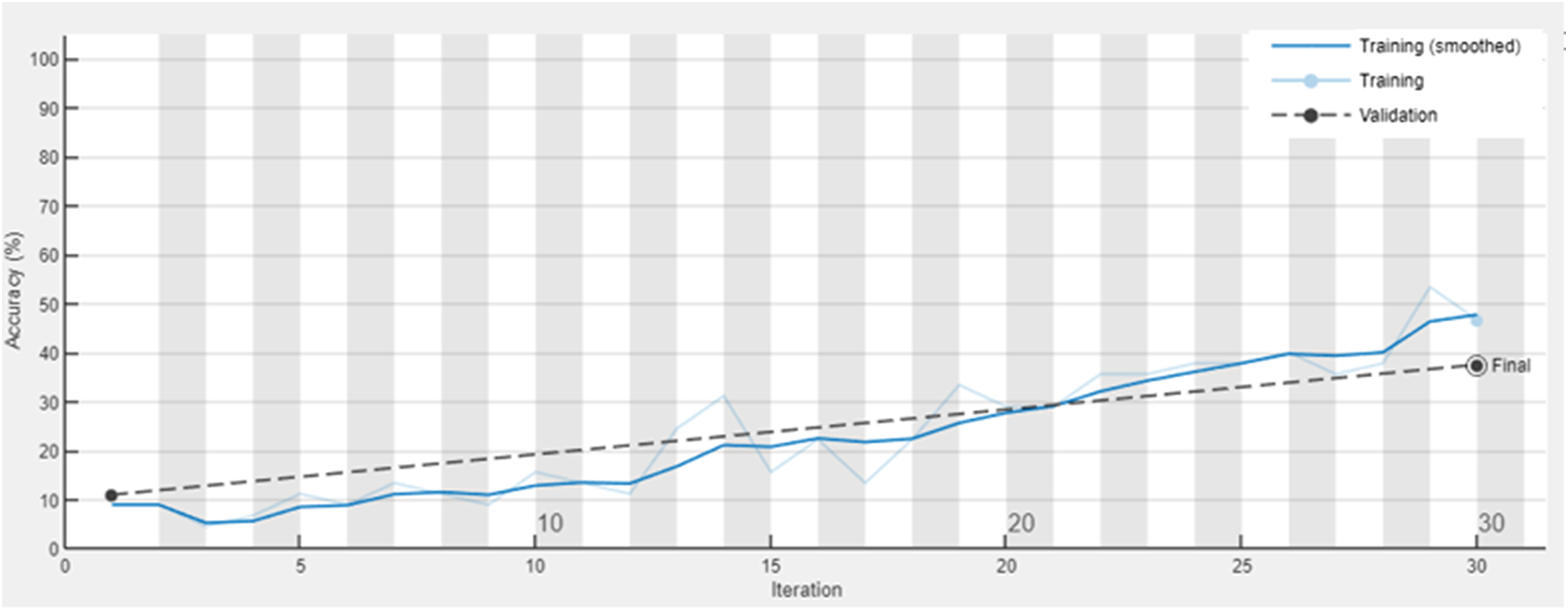

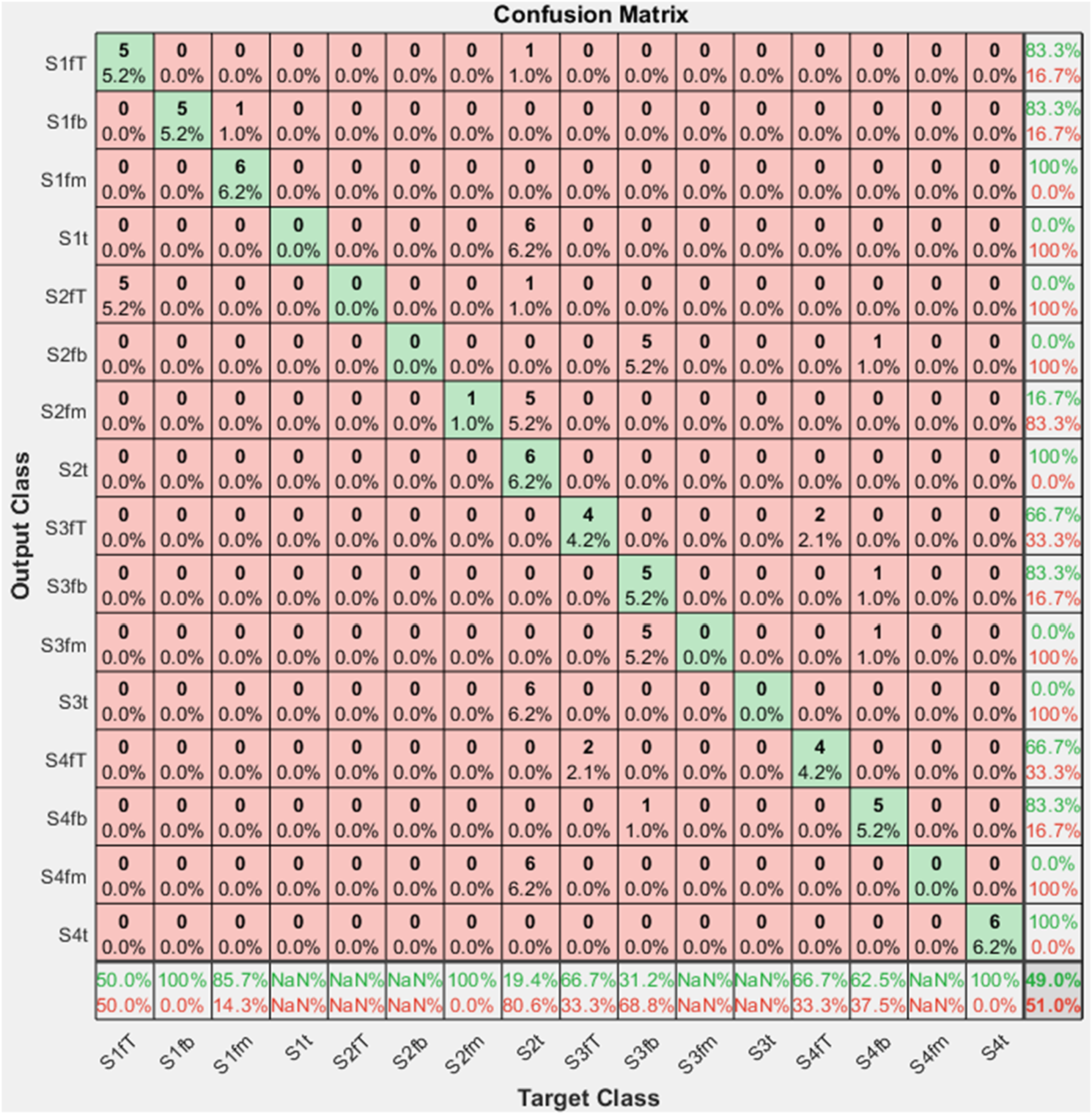
On the other hand, when the model is provided with the GASF images of dynamic displacements alone, the accuracy reaches 49% as shown in Figures 28 and 29. The prediction result highlights the model’s capacity to identify patterns within the vibrational signatures, although it still falls short of optimal performance.

Figure 28.

The training results using the GASF images of dynamic displacements as input.

Figure 29.

The confusion matrix using the GASF images of dynamic displacements as input.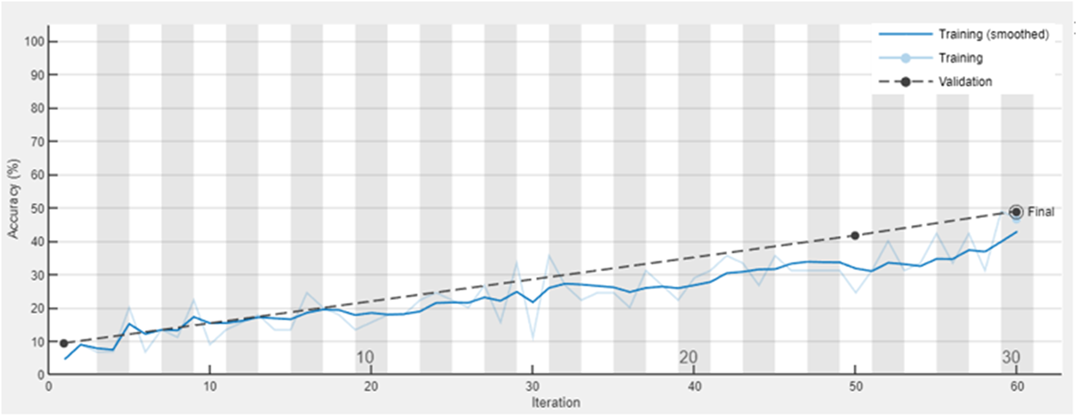

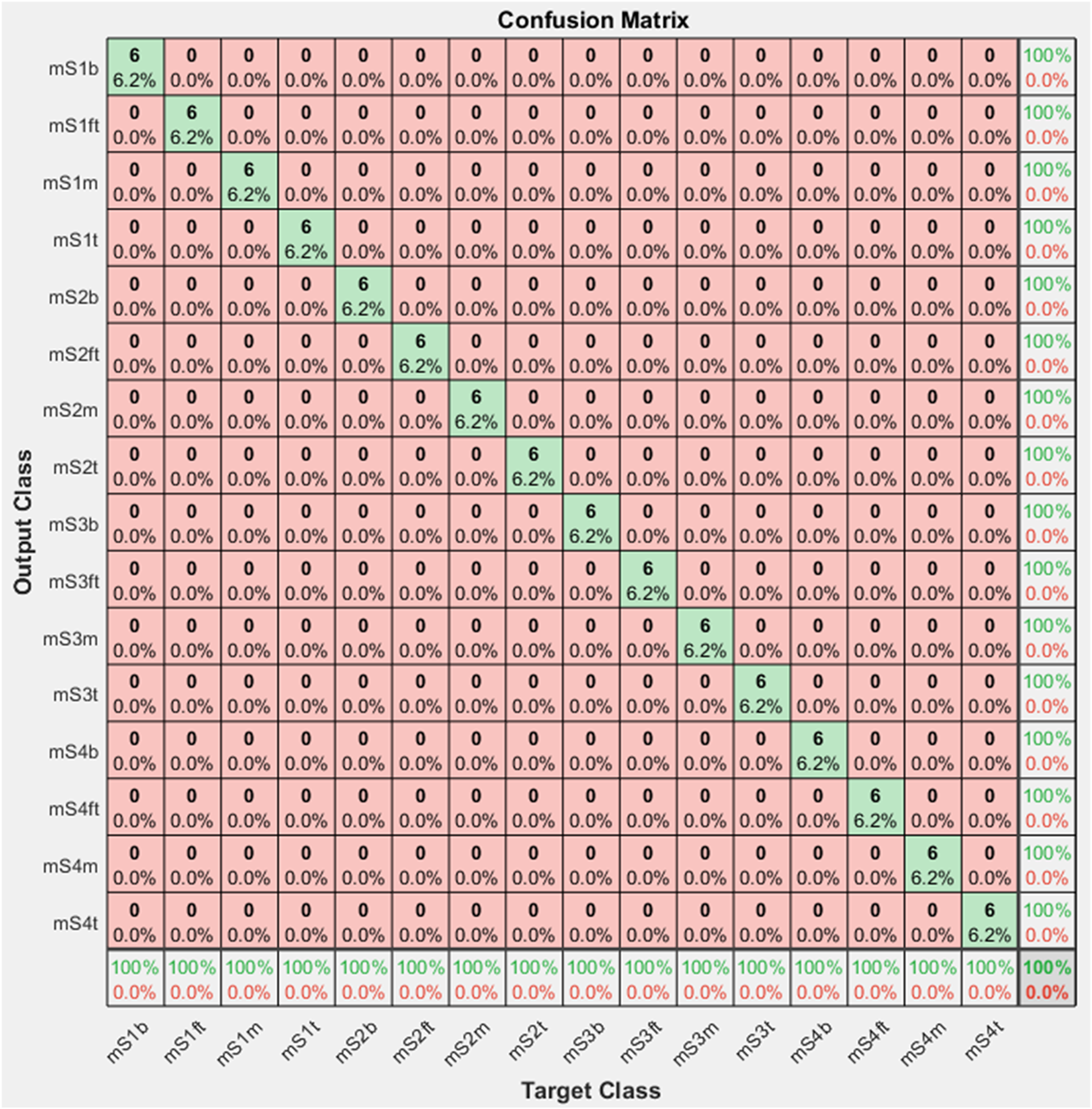
However, when the model is trained on the combined images of both GASF and optical structural damage photos, there is a dramatic change. In this multimodal approach, the GoogleNet model benefits from the complementary nature of both data types and demonstrates exceptional proficiency, achieving a perfect accuracy of 100% as shown in Figures 30 and 31. This remarkable result emphasizes the superior enhancement achieved by combining the GASF vibrational information with the optical truss images, demonstrating how a comprehensive approach can effectively capture the subtle patterns that are indicative of structural problems. The model’s performance in this integrated scenario highlights how multimodal data fusion can revolutionize the precision of structural health monitoring systems.

Figure 30.

The training results using images of combined optical truss photos and GASF vibration data as input.

Figure 31.

The confusion matrix using images of combined optical truss photos and GASF vibration data as input.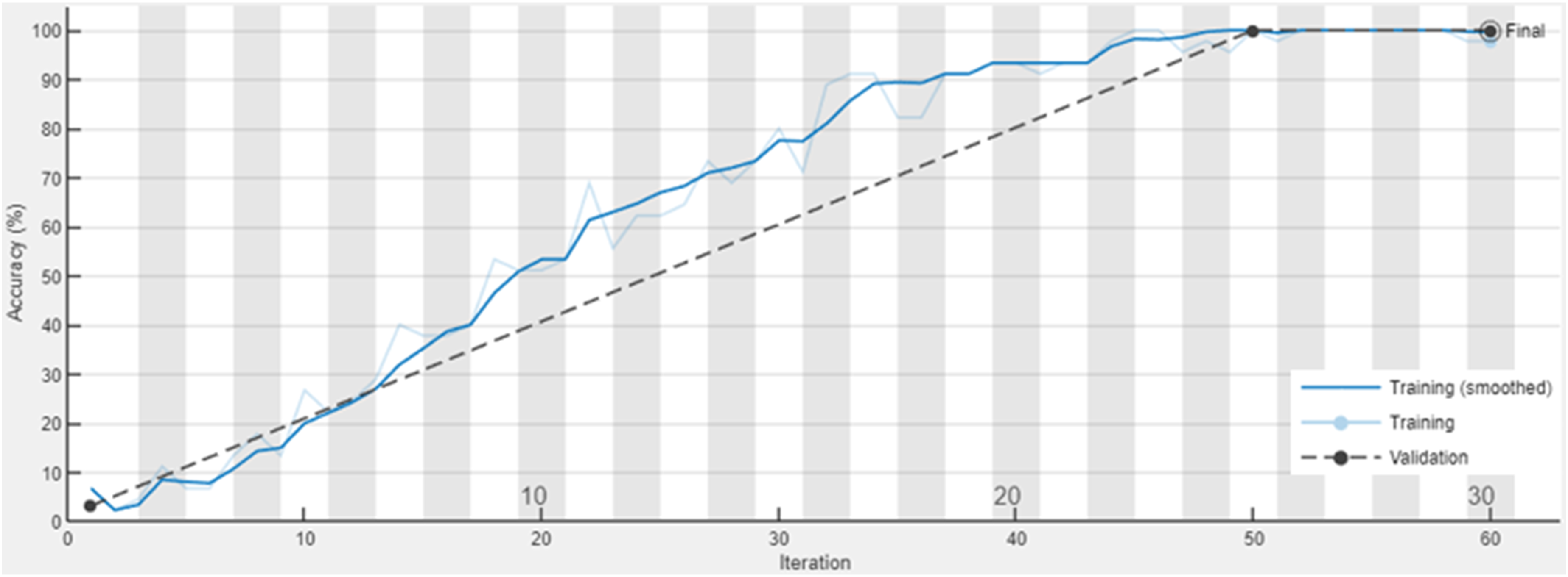

Conclusions

A beam and a steel truss ABAQUS model were used to provide inputs for the deep learning-based structural health monitoring method proposed in this paper. The effectiveness of deep learning models in vibration-based, image-based, and infusion of vibration and image data-based damage identification are summarized as follows:

• The proposed CNN-based method, trained by raw vibration data obtained in the ABAQUS models, has very high accuracy. This method classified different damages in the truss and beam cases accurately.

• The seven pretrained deep learning methods used in this paper had high accuracy, in which the ResNet101 model had the lowest accuracy at 95%. The Alex pretrained deep learning method is more effective because it has higher accuracy and less running time compared to the other six pretrained deep learning methods when they are trained by local crack photos.

• Integrating images using a defect photo and a converted GASF map provides richer information and would generate more accurate damage identification results.

In summary, vibration data or blurred optical photos alone can trigger false alarms, as shown in Figures 27 and 29. While the infusion of vibration signals and the optical damage image is a promising approach that can improve damage identification accuracy with early detection and precise localization of structural damage through partial and blurred target information, it still faces significant challenges like structure accessibility, weather conditions, cost and maintenance of sensing system as other conventional structural health monitoring methods do.

Footnotes

Declaration of conflicting interests

The author(s) declared no potential conflicts of interest with respect to the research, authorship, and/or publication of this article.

Funding

The author(s) disclosed receipt of the following financial support for the research, authorship, and/or publication of this article: This work was supported by the Aeronautics Research Mission Directorate (80NSSC19M0047).

ORCID iD

Mijia Yang

References

Adeli

Jiang

(2008) Intelligent Infrastructure: Neural Networks, Wavelets, and Chaos Theory for Intelligent Transportation Systems and Smart Structures. Boca Raton, FL: CRC Press, 305–332.

Al-Qudah

Yang

(2023) Large displacement detection using improved lucas–kanade optical flow. Sensors 23(6): 3152.

Al-Qudah

Yang

(2024) Effective hybrid structure health monitoring through parametric study of GoogLeNet. AI 5(3): 1558–1574.

Avci

Abdeljaber

Kiranyaz

, et al. (2018) Wireless and real-time structural damage detection: a novel decentralized method for wireless sensor networks. Journal of Sound and Vibration 424: 158–172.

Cawley

Adams

(1979) The location of defects in structures from measurements of natural frequencies. The Journal of Strain Analysis for Engineering Design 14(2): 49–57.

Chang

Kim

(2016) Modal-parameter identification and vibration-based damage detection of a damaged steel truss bridge. Engineering Structures 122: 156–173.

Chen

Jahanshahi

(2018) NB-CNN: deep learning-based crack detection using convolutional neural network and Naïve Bayes data fusion. IEEE Transactions on Industrial Electronics 65: 4392–4400.

Dorafshan

Maguire

Hoffer

, et al. (2017) Fatigue crack detection using unmanned aerial systems in under-bridge inspection. Idaho Department of Transportation 2: 1–120.

Ebrahimkhanlou

Farhidzadeh

Salamone

(2016) Multifractal analysis of crack patterns in reinforced concrete shear walls. Structural Health Monitoring 15: 81–92.

10.

Fan

Chen

, et al. (2020) Ensemble of deep convolutional neural networks for automatic pavement crack detection and measurement. Coatings 10: 152.

11.

Wang

Zhang

, et al. (2020) Automatic classification of pavement crack using deep convolutional neural network. International Journal of Pavement Engineering 21: 457–463.

12.

, et al. (2020) Automatic tunnel crack detection based on U-net and a convolutional neural network with alternately updated clique. Sensors 20: 717.

13.

Lin

Nie

(2017) Structural damage detection with automatic feature extraction through deep learning. Computer-Aided Civil and Infrastructure Engineering 32(12): 1025–1046.

14.

Liu

Cho

Spencer

BFJ

, et al. (2014) Automated assessment of cracks on concrete surfaces using adaptive digital image processing. Smart Structures and Systems 14: 719–741.

15.

Mao

Zhang

Qiao

, et al. (2022) Fusion domain-adaptation CNN driven by images and vibration signals for fault diagnosis of gearbox cross-working conditions. Entropy 24(1): 119.

16.

Rawat

Wang

(2017) Deep convolutional neural networks for image classification: a comprehensive review. Neural Computation 29: 2352–2449.

17.

Reynders

Wursten

De Roeck

(2014) Output-only fault detection in structural engineering based on kernel PCA. In: BIL2014 Workshop on Data-Driven Modeling Methods and Applications. Leuven, Belgium: KU-Leuven. 14–15 July.

18.

Soloviev

Sobol

Vasiliev

(2019) Identification of defects in pavement images using deep convolutional neural networks. Advanced Materials 4: 615–626.

19.

Tong

Gao

Han

, et al. (2018) Recognition of asphalt pavement crack length using deep convolutional neural networks. Road Materials and Pavement Design, 19, 1334–1349.

20.

Tran

Yang

, et al. (2013) Thermal image enhancement using bi-dimensional empirical mode decomposition in combination with relevance vector machine for rotating machinery fault diagnosis. Mechanical Systems and Signal Processing 38: 601–614.

21.

Wang

Song

, et al. (2019) A novel convolutional neural network based fault recognition method via image fusion of multi-vibration-signals. Computers in Industry 105: 182–190.

22.

Yan

Kerschen

De Boe

, et al. (2005) Structural damage diagnosis under varying environmental conditions. Part I: a linear analysis. Mechanical Systems and Signal Processing 19(4): 847–864.

23.

Yang

, et al. (2018) Automatic pixel-level crack detection and measurement using fully convolutional network. Computer-Aided Civil and Infrastructure Engineering 33: 1090–1109.

Deep learning-based structural health monitoring through the infusion of optical photos and vibration data

Abstract

Keywords

Introduction

Comparison of different deep-learning models using vibration signals

Deep learning-based damage detection using vibration data

Different pretrained deep learning methods used

Data collection through ABAQUS modeling

Results of model training, validation, and prediction

Results of crack detection using deep learning-based image classification

Structural evaluation using a novel deep-learning-based method with both defect image and vibration data

Gramian angular field

Flowchart of the proposed method

Results of the proposed method

Conclusions

Footnotes

Declaration of conflicting interests

Funding

ORCID iD

References