Sage Journals: Discover world-class research

Abstract

Due to the sheltering effect of the upper structures and the significant influence of temperature changes in the cables, the steel truss cable-stayed bridge with two-layer decks exhibits complex spatial thermal effects under solar radiation and environmental temperature. In order to study the temperature distribution characteristics and thermal deformation during the construction stage, the thermal effect of a steel truss cable-stayed bridge with two-layer decks under construction is analyzed through numerical simulation. Firstly, a temperature field analysis algorithm, which considers geo-meteorological factors and the sheltering relationship between members, was used to simulate the structure's transient temperature field and thermal deformation. Then, the temperature distribution characteristics and thermal deformation under the influence of seasons were discussed. The results indicated that the web members and the lower deck showed a significant temperature difference when shaded by the upper structure, with a maximum temperature difference of 7.6°C; The transverse temperature difference of the lower chord was the main factor controlling the transverse deformation of the steel truss girder; During a day in summer, the maximum vertical, longitudinal, and transverse deformations of the main members at the closure during the maximum single cantilever stage were 7.2 cm, 6.4 cm, and 5.9 cm, respectively.

Keywords

Steel truss cable-stayed bridge with two-layer decks heat-transfer analysis thermo-mechanical coupling model temperature distribution thermal deformation in construction

Introduction

Steel conducts heat quickly and is more sensitive to changes in environmental temperature. Under the influence of solar radiation and environmental temperature changes, the steel bridge will undergo significant temperature changes. (Chen, 2008; Liu et al., 2016; Wang et al., 2017). The structural temperature variations and inhomogeneities may significantly alter the static and dynamic performance of the bridge, which increases the bridge design and construction difficulty (Roeder, 2003; Xia et al., 2012). When the bridge is completed and opened to traffic, the negative impact of temperature changes on the bridge is even greater than the vehicle load (Catbas et al., 2008; Priestley, 1976; Tong et al., 2001; Xia et al., 2017).

Currently, the research methods for thermal effects of bridge structures mainly include numerical simulation and experimental testing (Li et al., 2023; Zhou and Yi, 2013). Compared to numerical simulation, the data obtained from experimental testing is more authentic and reliable. Therefore, some scholars use this method to study the bridge's temperature distribution and temperature response. Based on the measured temperature data of a constructed composite box-girder bridge for about 20 months, Chang and Im (2000) defined major thermal loading parameters that characterize the temperature profile, and detailed the seasonal behavior of these parameters. Roberts-Wollman et al. (2002) monitored temperature on a concrete box girder bridge for two and a half years, and presented equations to predict positive temperature differentials. Xu et al. (2010) analyzed the temperature characteristics of the Tsing Ma Bridge using years of monitoring data. Ding et al. (2012) proposed a critical temperature difference models in cross-section for thermal stress calculation through relevant analysis of long-term monitoring data of flat steel box girder bridge. As for the steel truss cable-stayed bridge with two-layer decks, Wang et al. (2021) conducted corresponding research. The long-term monitoring data of the Zhengzhou Yellow River Bridge revealed a significant temperature difference between the steel trusses. However, there are still some problems in studying the thermal effects of bridges through actual measurements. Firstly, there are few cross-sectional measurement points arranged, and the obtained temperature data is difficult to directly apply to the design calculation of bridges; Secondly, it is hard to obtain the temperature effect of the bridge structure. Therefore, using precise numerical simulation methods is still an important supplement to grasp the spatial temperature field and temperature effects of complex bridges.

Many scholars have conducted the finite element simulation of the bridges with simple structures in the form of calculating thermal boundary conditions. Emanual and Hulsey (1978) calculated the temperature variation over time of a highway composite beam bridge. Chen (2008) conducted a long-term finite element simulation of the temperature field of composite beams for 45 years and obtained sufficient temperature action samples for extreme value analysis. Zhou et al. (2016b) determined the initial thermal conditions of the model through pre-analysis, and then carried out transient heat transfer analysis to investigate the vertical and transverse temperature differences of the steel box girder. For rapid calculation of temperature loads, Fan et al. (2022) deduced and established vertical discrete and dimensionality-reduced model of a steel–concrete composite bridge. At the same time, outdoor sunlight experiments were conducted to study the temperature field. In addition, for the first time, Shan et al. (2023) integrated heat transfer analysis and field monitoring data, and established a 3D finite element model of a navigation channel bridge of the Hong Kong‒Zhuhai‒Macao Bridge, comprehensively and accurately studying the global 3D temperature distribution of the long-span cable-stayed bridge. Although many studies have been conducted, there is still a lack of research on the numerical simulation of long-span steel truss bridge. The reason for this is the difficulty of dynamically identifying shaded areas due to bridge components and terrain obstruction (Liu et al., 2019). For this purpose, Yin et al. (2014) compiled an ANSYS subroutine using ray tracing method to accurately simulate the main beam's covering effect on the concrete arch. bridge's arch. box. Zhu and Meng (2017) proposed a three-dimensional (3D) sunlight-sheltering algorithm based on a sun ray tracing method and applied the substructure method to thermo-mechanical coupling analysis, accurately predicting the temperature field and temperature effects of cable-stayed bridges. Zhu et al. (2023) calculated the sunlight shadow coefficient between different members using the bounding box algorithm and the elimination algorithm to simulate the non-uniform temperature field caused by occlusion between components.

In summary, for the temperature field of simple structure bridge, its numerical simulation technology has been more complete. However, for the steel truss bridge with two-layer decks, a long-span bridge with complex structures, the solution of the exact temperature field is still lacking. The problem is that the dynamic identification of shadow areas caused by bridge members is difficult. On the one hand, in solving the non-uniform temperature field caused by sunlight, it is difficult to identify the shadow areas caused by bridge members dynamically. This article calculates the thermal boundary conditions of a steel truss cable-stayed bridge with two-layer decks based on geo-meteorological factors, and employs a three-dimensional ray occlusion algorithm to identify its shadow area dynamically. During this period, the mutual sheltering effect of the upper deck on the web member, the upper deck and the web member on the lower deck is considered. Finally, the simulation of the transient temperature is achieved. On the other hand, when solving the thermal deformation of a steel truss cable-stayed bridge with two-layer decks, only the influence of uniform temperature field is generally considered. Therefore, based on the non-uniform temperature field simulated above and considering the temperature changes of the cables, this article establishes a thermo-mechanical coupling model to analyze the thermal deformation at the closure during the maximum single cantilever construction stage.

Thermal analysis method for bridge structures

Thermal environment of steel truss

The temperature distribution of the bridge structure under sunlight is basically determined by both internal heat transfer and external heat exchange. The internal heat conduction is controlled by the Fourier heat transfer equation. As for the conditions for the solution of the three-dimensional transient heat transfer partial differential equation, instantaneous temperature and boundary conditions are included (Lienhard and Lienhard, 2003). As shown in Figure 1, the heat exchange between the bridge and the external natural environment under sunlight includes three forms: solar radiation, convective heat transfer with the atmospheric environment, and radiation heat transfer on the structural surface.

Figure 1.

Heat exchange diagram with external environment: (a) The spatial relationship between the bridge and sun; (b) Heat exchange between the main girder and the external environment.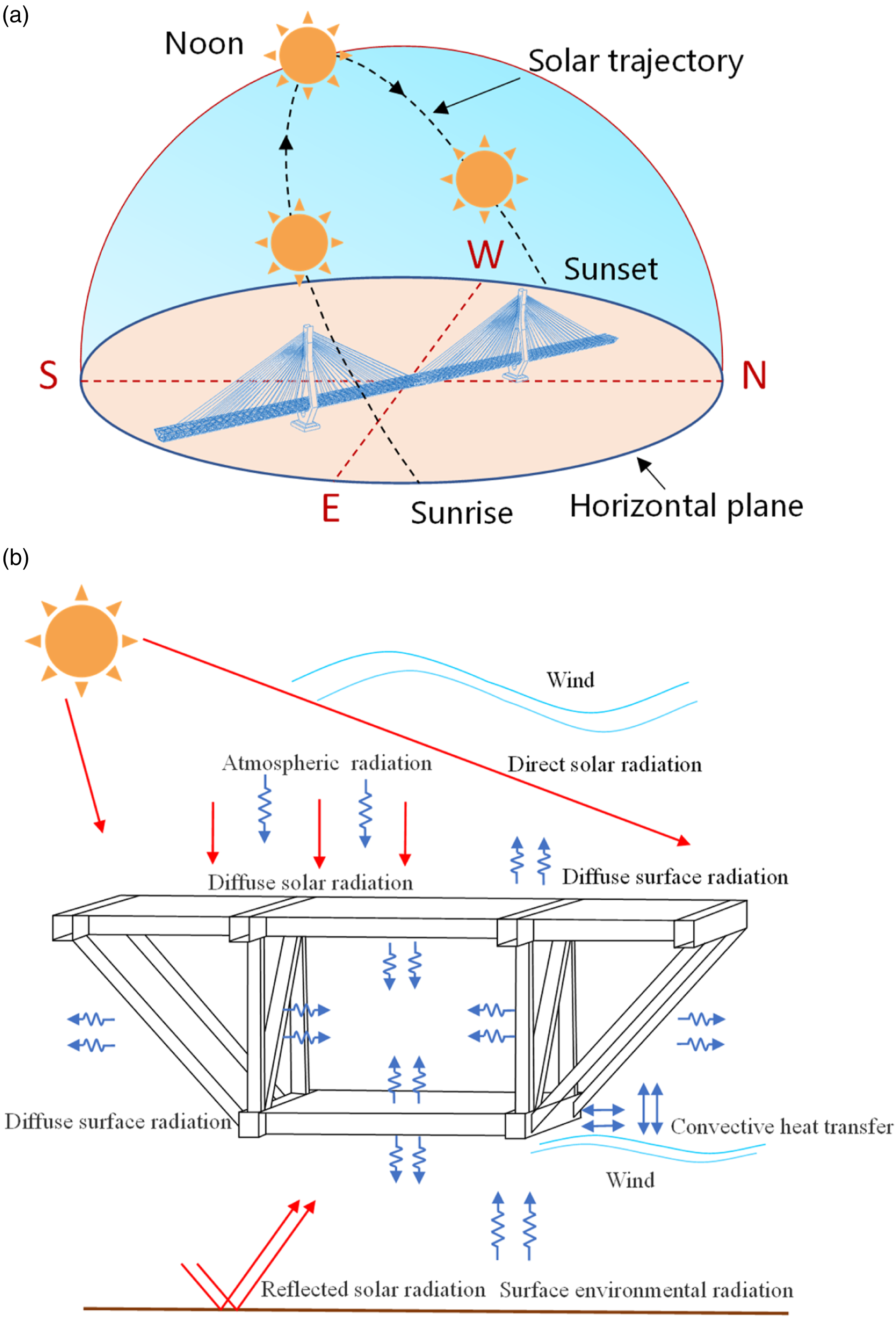

Heat-Transfer Analysis

Heat-Transfer theory

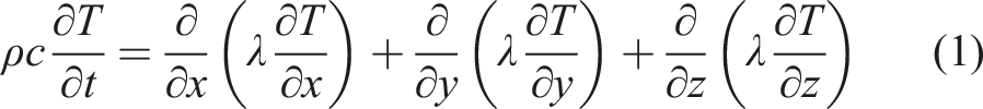
The internal heat transfer of the bridge structure follows Fourier's law, and the three-dimensional transient heat transfer partial differential equation is presented in equation (1):

ρ c \frac{\partial T}{\partial t} = \frac{\partial}{\partial x} (λ \frac{\partial T}{\partial x}) + \frac{\partial}{\partial y} (λ \frac{\partial T}{\partial y}) + \frac{\partial}{\partial z} (λ \frac{\partial T}{\partial z})

(1)

where T = T (x, y, z, t) = Temperature at a point of the bridge structure; x, y, and z = Cartesian coordinates of the point and t = time;

ρ

= density; c = specific heat; and λ = thermal conductivity of the material.

Thermal Boundary Conditions

The thermal boundary conditions are generally divided into three types (Lienhard and Lienhard, 2003). Based on the known ambient temperature $T_{a}$ and comprehensive heat transfer density q around the bridge, the three-dimensional temperature field of the structure can be solved by applying the third type boundary condition of the equation. The comprehensive heat transfer density with the external environment can be expressed as follows:

q = q_{s} + q_{c} + q_{r}

(2)

Where

q_{s}

q_{c}

q_{r}

= the heat flow density of solar radiation, convective heat transfer, and radiation heat transfer respectively.

During the process of sunlight passing through the atmosphere and reaching the earth's surface, it is continuously affected by various atmospheric components, such as absorption, reflection, and scattering. This is called solar radiation, which consists of direct, diffuse, and reflected solar radiation.

Direct solar radiation

Attenuated by the atmosphere, the solar radiation reaching the structure's surface is direct solar radiation $I_{d}$ . According to the power index model proposed by Kehlbeck (1981), the $I_{d}$ on the horizontal surface is shown as follows:

I_{d} = I_{0} P^{m}

(3)

Where

I_{0}

= solar constant (W/

m^{2}

); m = atmospheric optical mass, which is equal to the cosecant of solar altitude; p = atmospheric transparency coefficient, which can be calculated using

P = {0.9}^{t_{u} k_{a}}

(Chen, 2008),

t_{u}

= turbidity coefficient,

k_{a}

= relative atmospheric pressure.

If the surface is inclined, the direct solar radiation can be expressed as follows:

I_{d φ} = I_{d} \cos φ

(4)

Where

φ

= solar incident angle.

Diffuse solar radiation

Scattered by air, aerosol molecules, and other particles, the solar radiation reaching the structure's surface is diffuse solar radiation $I_{r}$ . The $I_{d}$ on the horizontal surface is determined as follows (Li, 1996):

I_{r} = 0.5 I_{0} \frac{1 - P^{m}}{1 - 1.4 \ln P} \sin (β_{s})

(5)

Where

β_{s}

= the solar altitude angle.

If the surface is inclined, the diffuse solar radiation can be expressed as follows:

I_{r β} = \frac{1 + \sin (β_{n})}{2} I_{r}

(6)

Where

β_{n}

= the angle between the normal vector of the surface and the ground plane.

Reflected solar radiation

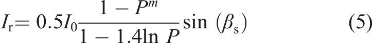
The portion of direct and scattered solar radiation, which reaches the ground (water) surface and is reflected on the bridge's surface, is called reflected solar radiation $I_{f}$ . The $I_{f}$ on the horizontal surface can be calculated as follows (Li, 1996):

I_{f} = R_{e} [I_{d} \sin (β_{s}) + I_{r}]

(7)

Where

R_{e}

= short-wave radiation coefficient, taking 0.2 for ordinary ground and 0.6 to 0.8 for water surface.

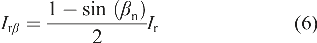
If the surface is inclined, the reflected solar radiation can be expressed as follows:

I_{f β} = \frac{1 - \sin (β_{n})}{2} I_{f}

(8)

Overall, the total solar radiation heat flux density that the surface of the bridge structure can absorb is shown as follows:

q_{s} = α (I_{d φ} + I_{r β} + I_{f β})

(9)

Where

α

= short-wave radiation coefficient of material.

Differing from solar radiation, which is short-wave radiation, the essence of radiation heat transfer is electromagnetic radiation generated by heat, belonging to long-wave radiation. It absorbs radiation from the atmosphere and surface and releases radiation toward the surrounding environment. It includes atmospheric radiation, surface environmental radiation, and diffuse surface radiation.

Atmospheric radiation

The atmosphere radiates energy outward by its temperature, and the part returned to the ground (water) surface is called atmospheric reverse radiation $I_{a}$ . The $I_{a}$ on the horizontal surface is shown as follows (Kehlbeck, 1981)

I_{a} = ε_{sa} C_{0} {(T_{a} + 273.15)}^{4}

(10)

Where

ε_{sa}

= atmospheric radiation coefficient, usually taken as 0.82;

C_{0}

= Stefan-Boltzmann constant, taken as 5.67×

10^{- 8}

W (

m^{2}

K^{4}

);

T_{a}

= ambient temperature.

If the surface is inclined, the atmospheric radiation can be expressed as follows:

I_{a β} = \frac{1 + \sin (β_{n})}{2} I_{a}

(11)

Surface environmental radiation

The radiation caused by the exchange of energy between the ground (water) surface and the bridge surface is called surface environmental radiation $I_{g}$ . The $I_{g}$ on the horizontal surface is determined as follows (Kehlbeck, 1981):

I_{g} = C_{0} {(T_{g} + 273.15)}^{4}

(12)

Where

T_{g}

= ground (water) surface temperature, usually

T_{g}

T_{a}

(Lee and Kalkan, 2012).

If the surface is inclined, the atmospheric radiation can be expressed as follows:

I_{g β} = \frac{1 - \sin (β_{n})}{2} I_{g}

(13)

Diffuse surface radiation

The radiation emitted by the bridge surface in the form of electromagnetic waves is called diffuse surface radiation $I_{s}$ . The $I_{s}$ can be calculated as follows (Kehlbeck, 1981)

I_{s} = ε_{s} C_{0} {(T_{s} + 273.15)}^{4}

(14)

Where

ε_{s}

= emissivity of concrete or steel surface;

T_{s}

= structural surface temperature.

Thus, the radiation heat flux density $q_{r}$ during the heat transfer process between the bridge and the external environment is shown as:

q_{r} = ε_{r} (I_{a β} + I_{g β}) - I_{s}

(15)

Where

ε_{r}

= long-wave absorptivity of concrete or steel surface, which is the same as the emissivity

ε_{s}

The heat flow of Convective heat transfer is calculated by Newton's heat transfer equation:

q_{c} = h_{c} (T_{a} - T)

(16)

where

T_{a}

= external ambient temperature;

T

= bridge surface temperature;

h_{c}

= convection heat transfer coefficient, When the wind speed is small, the convective is given as follows (Kehlbeck 1981):

h_{c} = 2.6 (\sqrt[4]{T_{a} - T} + 1.54 v)

(17)

Three-dimensional ray sheltering theory

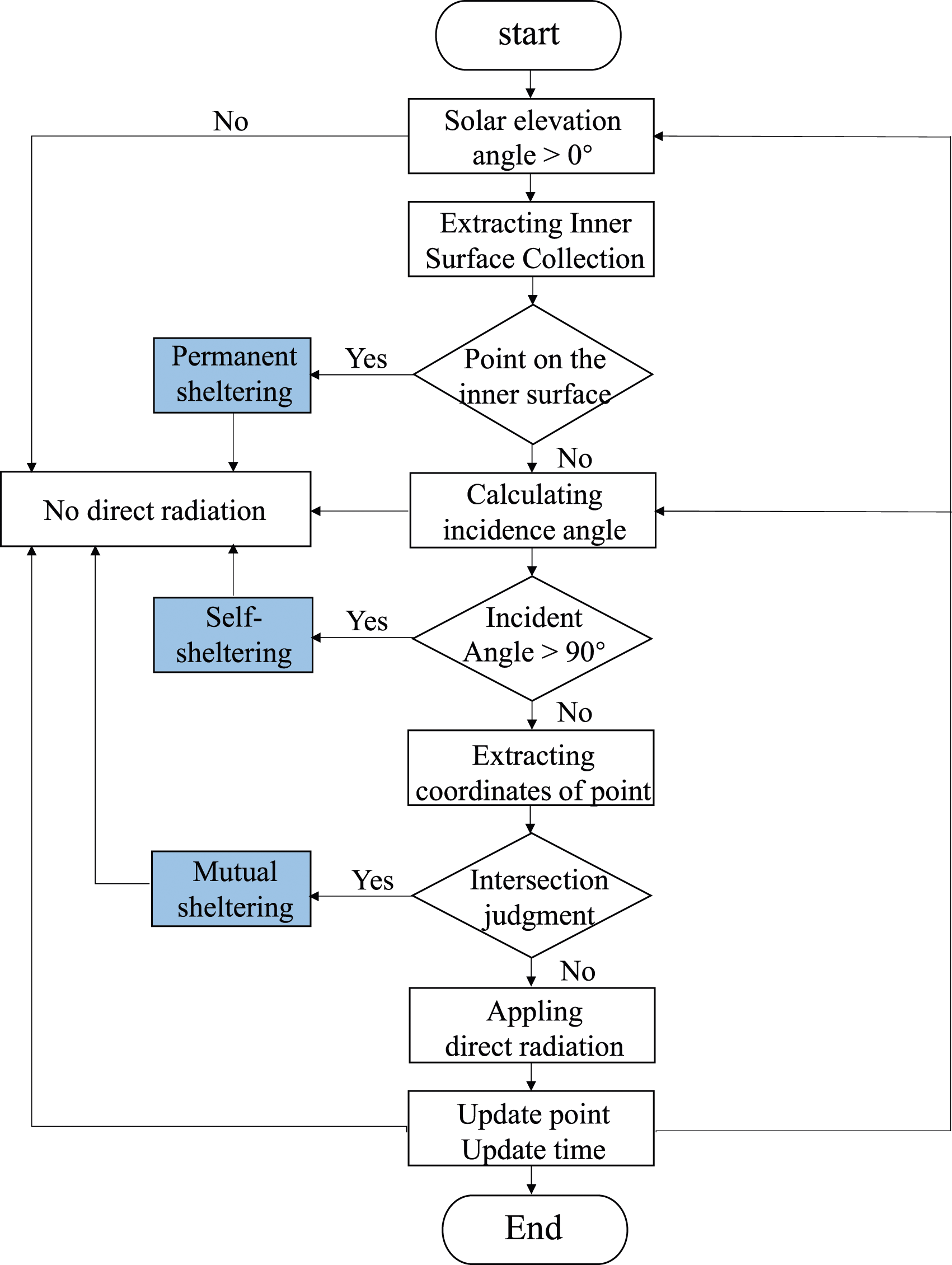
Due to the motion of the sun, some surfaces of the bridge will be in shadow, and the thermal boundary conditions of that surface will also be affected. As shown in Figure 2, the conditions for generating shadows contain the following three types. Firstly, if the connection between the bridge surface and the sun passes through its own structure at any time, then the surface is in a permanent sheltering state. Secondly, if there is some time when the solar incident angle is greater than 90°, then the surface is in a self-sheltering state. Thirdly, if the bridge does not belong to the above two sheltering states, but is unable to be directly radiated by the sun due to the obstruction of other surfaces, then the surface is in a mutual sheltering state. The specific algorithm implementation process is given in Figure 3 (Meng, 2019).

Figure 2.

Schematic diagram of three types of sheltering.

Figure 3.

Flowchart of the 3D sheltering algorithm.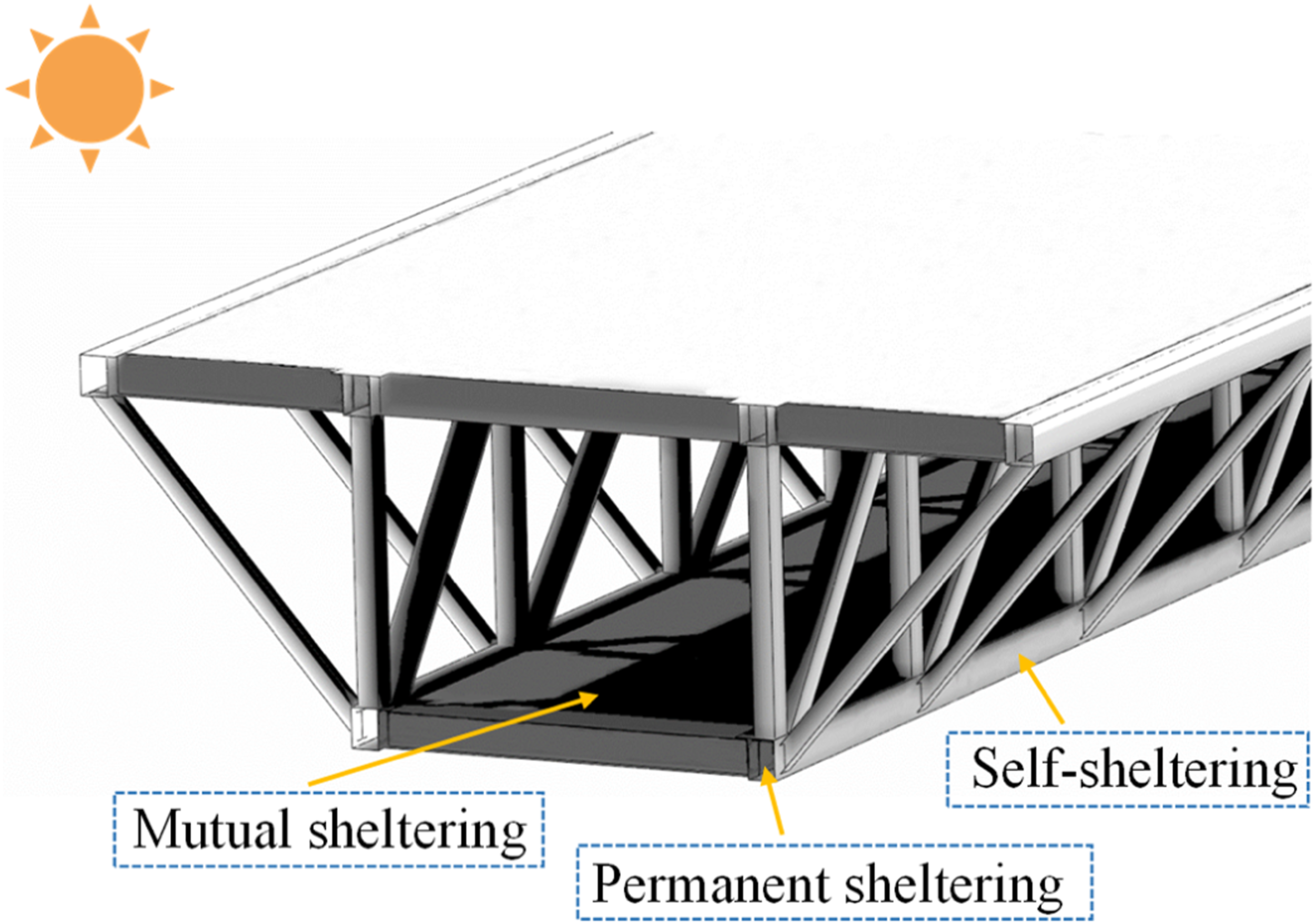

Initial temperature filed

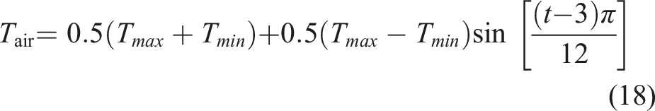
When simulating the temperature field, the selection of the initial temperature field must be considered. Commonly, it is assumed that the initial temperature of the bridge is uniform. The ambient temperature at 3:00 before sunrise is employed as the initial value for the numerical simulation of the bridge, and this temperature is regarded as the lowest value. Then, through several days of cyclic calculation, errors caused by the initial value selection are eliminated. (Kim et al., 2015; Moorty and Roeder, 1992). This study calculated the temperature changes of a steel truss cable-stayed bridge with two-layer decks and found that the temperature showed periodic changes starting from the third day. The variation in air temperature is expressed as follows:

T_{air} = 0.5 (T_{\max} + T_{\min}) + 0.5 (T_{\max} - T_{\min}) \sin [\frac{(t - 3) π}{12}]

(18)

Where

T_{air}

= air temperature varying with time t;

T_{\max}

and

T_{\min}

= maximum and minimum air temperature.

Numerical analysis and validation

Numerical analysis process

The analysis process of the thermal effect of the bridge mainly includes two parts, the solution of transient temperature field and thermal deformation. The transient temperature field is solved using the DFLUX and FILM subroutine modules in the finite element software ABAQUS. The subroutine simulates the process of solar motion based on the geo-meteorological information of the area where the bridge is located. It also simulates its radiation intensity in view of thermal boundary conditions and 3D sheltering algorithm. For thermal deformation analysis, a thermo-mechanical coupling model is established according to the temperature field obtained from the previous calculation.

Validation

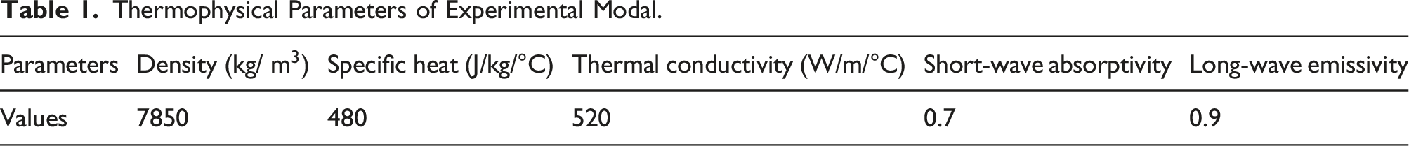
To verify the above theory and analysis process, numerical simulation was conducted on the temperature field of a steel truss cable-stayed bridge spanning the Yangtze River in Jiangsu Province, China. And compared with the measured temperature values from July 22 to July 23, 2022 (Zhu et al., 2023). The main span of the bridge is 1092m, located at 119.69° E and 32.23° N, with an azimuth angle of 73° northwest. The thermophysical parameters of the steel used are presented in Table 1.

Table 1.

Thermophysical Parameters of Experimental Modal.

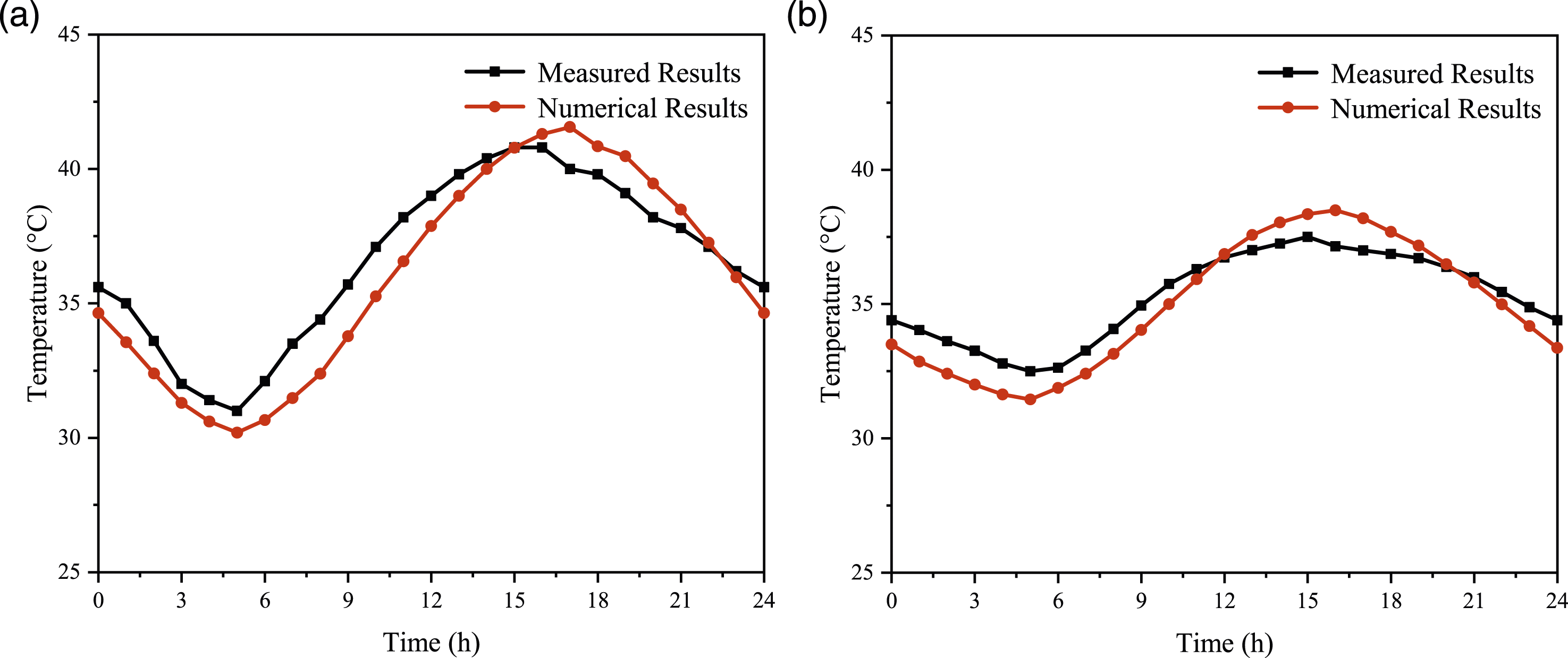
Parameters	Density (kg/ $m^{3}$ )	Specific heat (J/kg/°C)	Thermal conductivity (W/m/°C)	Short-wave absorptivity	Long-wave emissivity
Values	7850	480	520	0.7	0.9

The temperature distribution of the section where the temperature measuring points are located is shown in Figure 4. Here, the shadow appeared at the lower deck because of the obstruction of the upper deck and web members. The selected temperature measuring points included points 1 and 2 on the lower chord, and measuring points 3 and 4 on the lower deck. Take the average value of points 1 and 2 as the actual measuring result of the lower chord, and the average value of points 3 and 4 as the actual measuring result of the lower deck. The measuring result and the numerical result are plotted in Figure 5. Through comparison, the trend of the two changes was the same, and the data was in good agreement. The maximum error was 1.8°C, which meets the accuracy requirements of actual engineering.

Figure 4.

Temperature distribution and shadow region.

Figure 5.

Measured and simulated temperatures of the bridge for July 22,2022. (a) Lower chord;(b) Lower deck.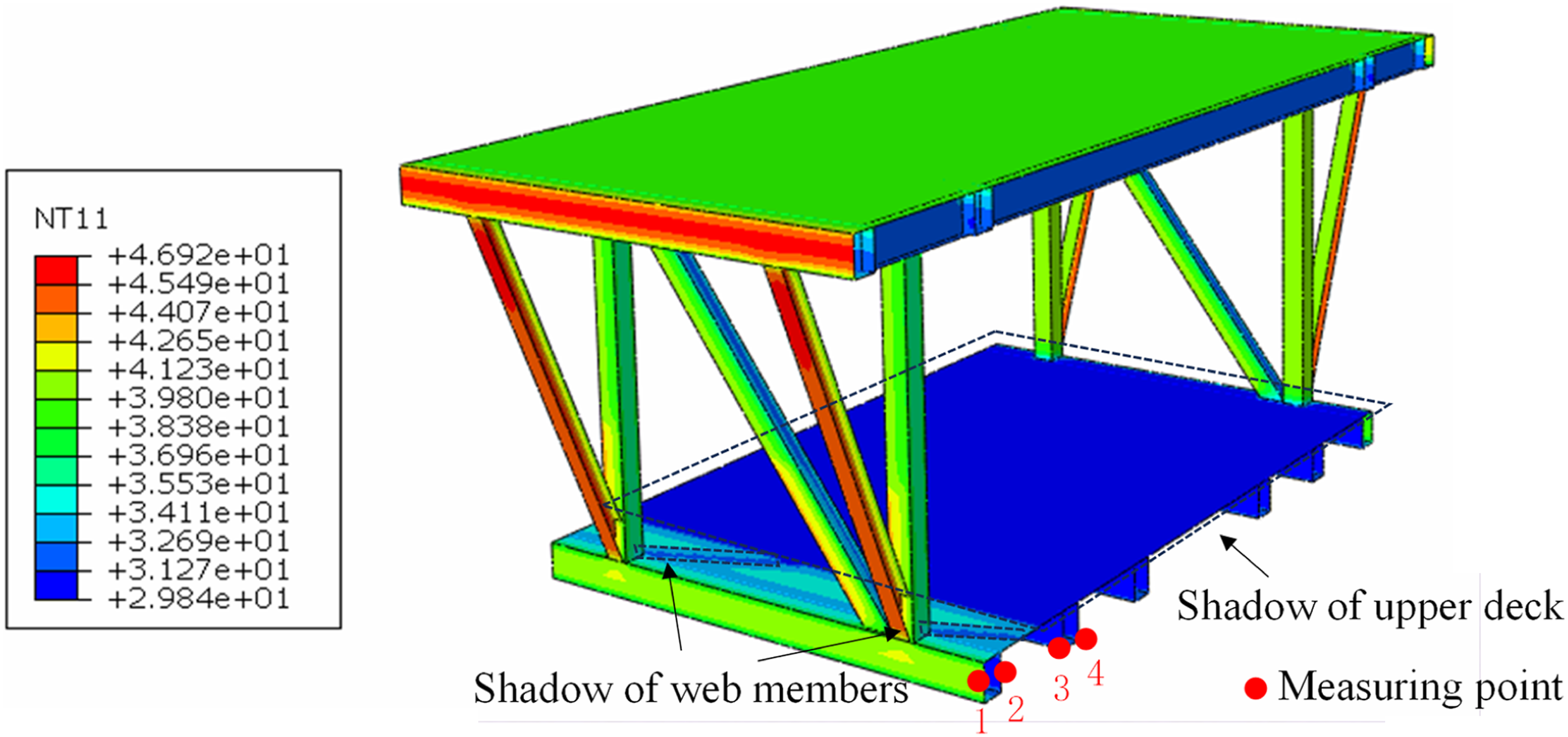

Case

Description of experimental bridge

The thermal effect analysis was conducted on an ongoing steel truss cable-stayed bridge with two-layer decks, spanning the Yellow River in Jinan, China. The bridge has a 1028m-long (90 + 180+488 + 180 + 90) steel truss girder, a 37.5m-wide upper deck and a 15m-wide lower deck. It is located at 116.1° E, 39.2° N, and has an azimuth angle of 8.8° northwest. Figure 6 shows the basic information of the experimental bridge location. The bridge crosses the Yellow River, and the surrounding terrain is flat. No mountains or high-rise buildings are blocking the sunlight.

Figure 6.

Experimental bridge.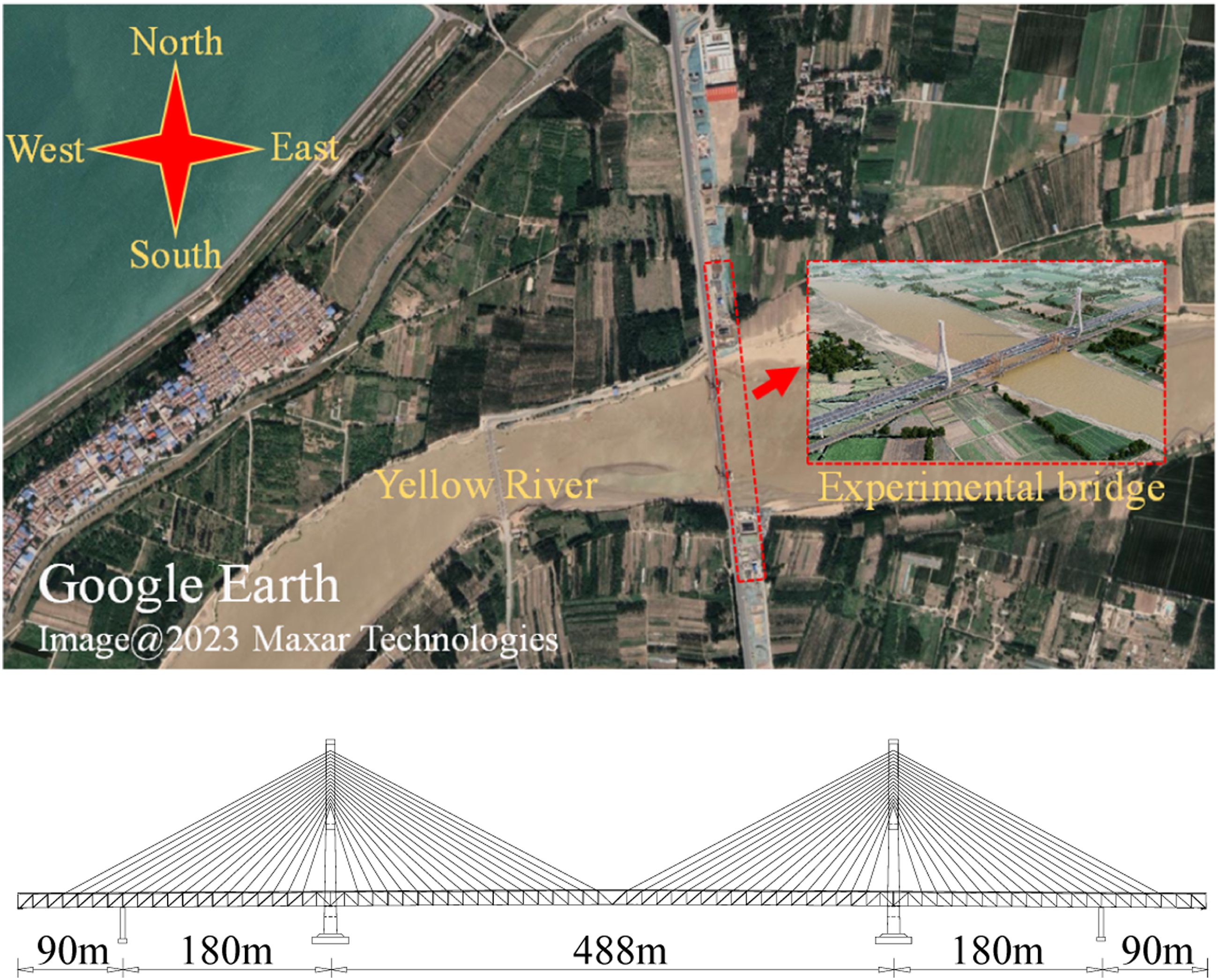

The main girder of this bridge is composed by two-layer decks. As shown in Figure 7, the main girder consists of the upper chord (M₂ and M₃), lower chord (M₅ and M₆), side girder (M₁ and M₄), web members, inclined strut, upper deck system, and lower deck system. For the convenience of subsequent discussions, Figure 7 also represents the sun’s exposure to the steel truss girder at sunrise and sunset.

Figure 7.

Cross-section of the main girder.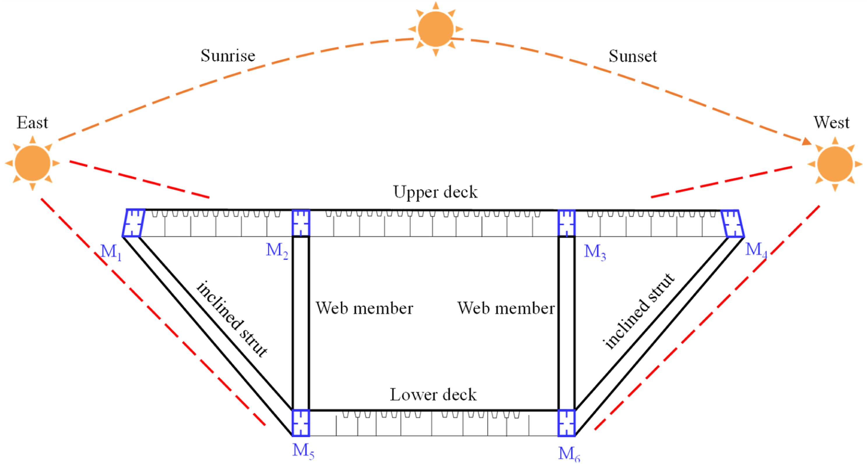

Finite element simulation

The finite element software ABAQUS was employed to study the transient temperature field and thermal deformation. The flow chart is presented in Figure 8. The primary analysis step was to use DFLUX and FILM subroutine interfaces for the secondary development of finite element software ABAQUS, during which a three-dimensional occlusion algorithm was used to identify shadow areas and accurately simulate the heat exchange between the structure surface and the external environment.

Figure 8.

Flow chart for temperature field simulation.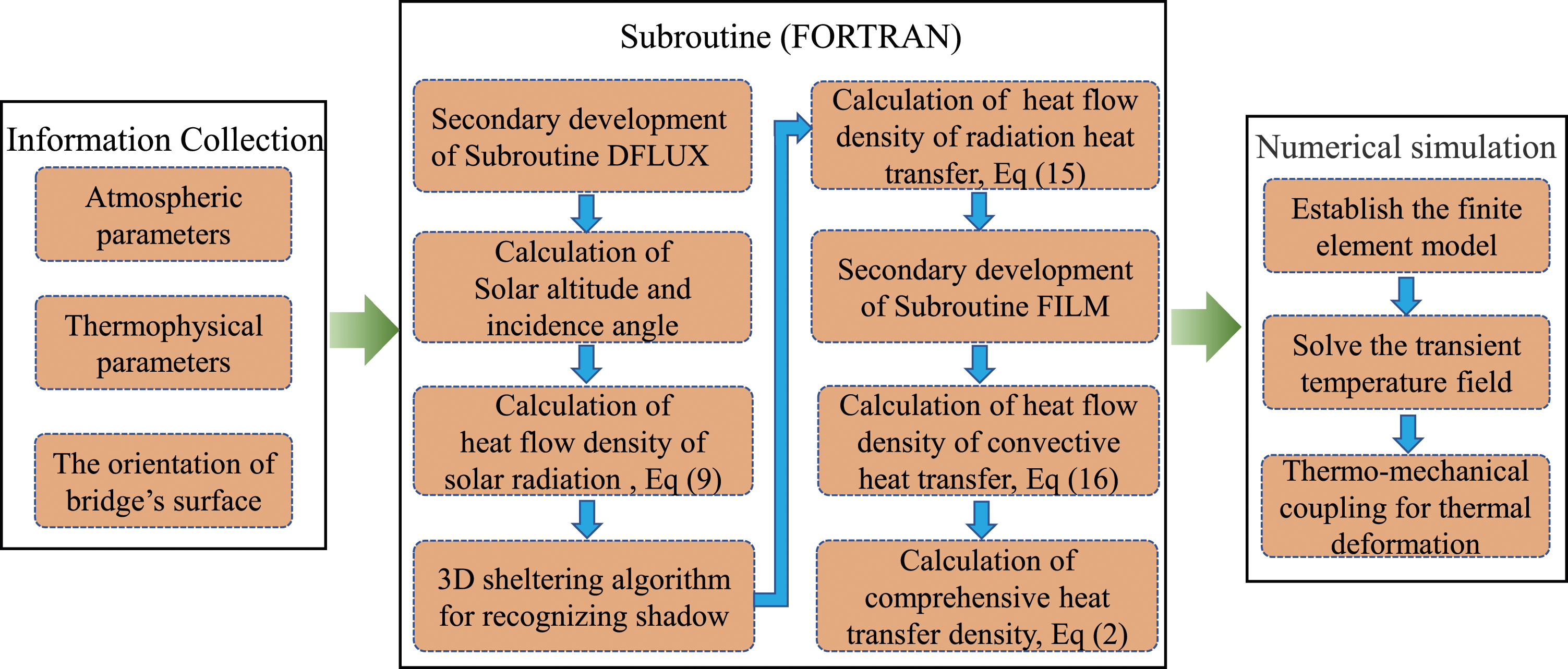

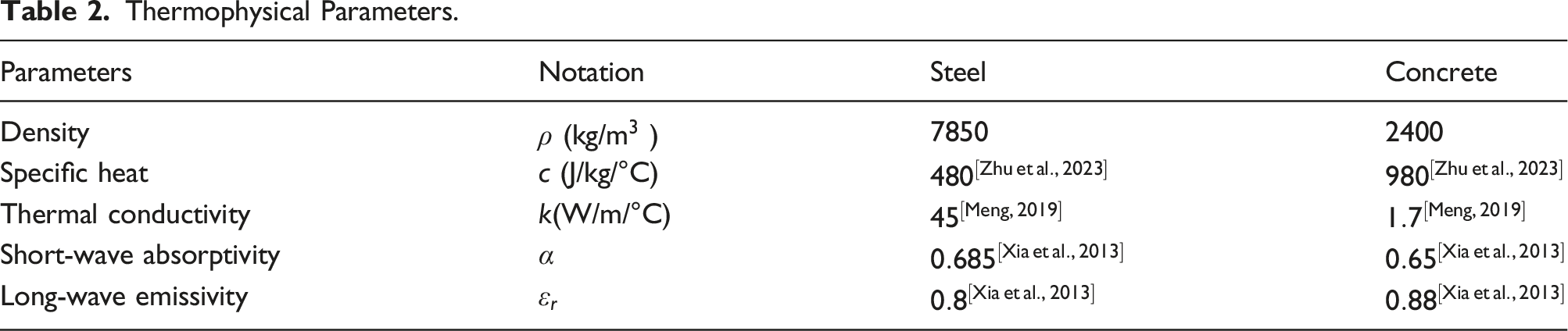
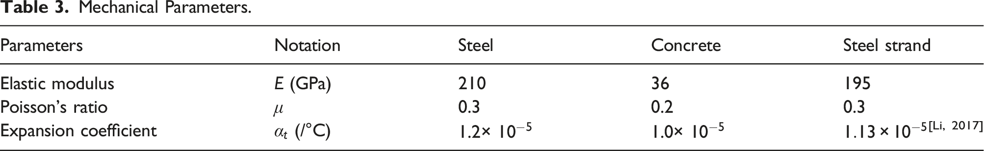
Figure 9 shows the established finite element model of a steel truss cable-stayed bridge with two-layer decks. In the heat transfer analysis, Shell (DS4) element was utilized for the steel truss girder, and Solid (DC3C8) was utilized for the bridge tower. When calculating thermal deformation, the elements used for steel, concrete, and cables were Shell (S4R), Solid (C3D8R), and Truss (T3D2), respectively. Tables 2 and 3 list the thermophysical and mechanical parameters.

Figure 9.

Finite element model.

Table 2.

Thermophysical Parameters.

Parameters	Notation	Steel	Concrete
Density	$ρ$ (kg/ $m^{3}$ )	7850	2400
Specific heat	c (J/kg/°C)	$480^{[Zhu et al ., 2023]}$	$980^{[Zhu et al ., 2023]}$
Thermal conductivity	k(W/m/°C)	$45^{[Meng, 2019]}$	${1.7}^{[Meng, 2019]}$
Short-wave absorptivity	$α$	${0.685}^{[Xia et al ., 2013]}$	${0.65}^{[Xia et al ., 2013]}$
Long-wave emissivity	$ε_{r}$	${0.8}^{[Xia et al ., 2013]}$	${0.88}^{[Xia et al ., 2013]}$

Table 3.

Mechanical Parameters.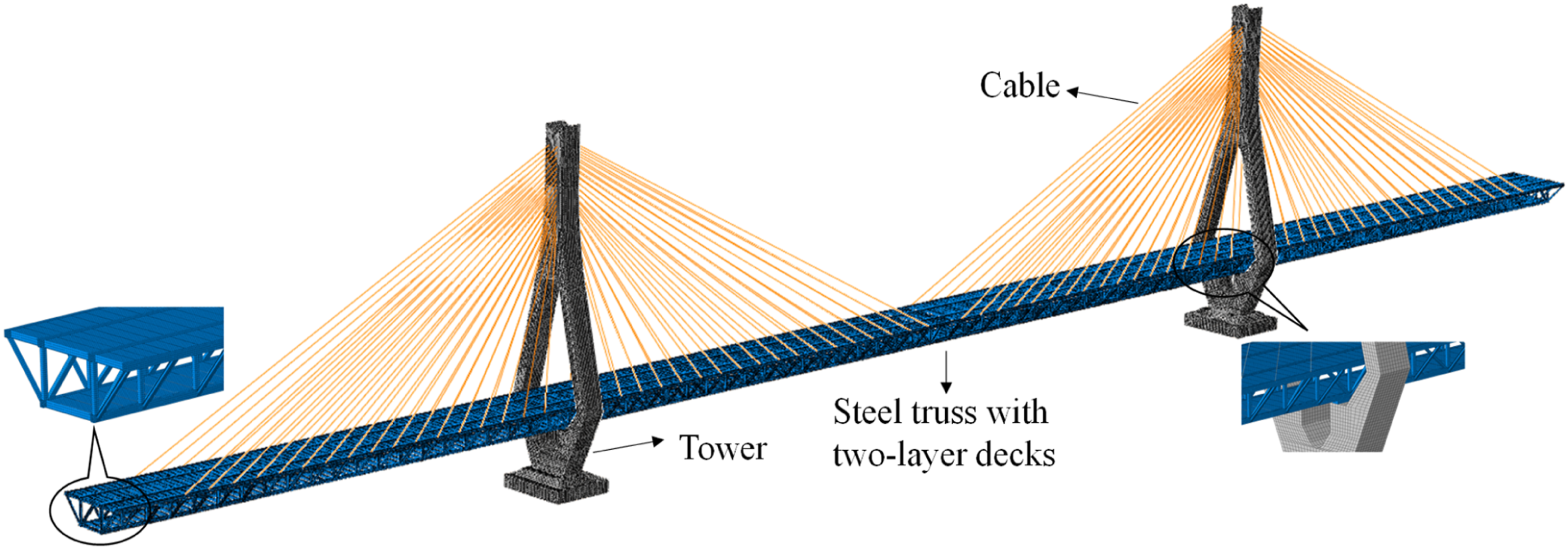

Parameters	Notation	Steel	Concrete	Steel strand
Elastic modulus	E (GPa)	210	36	195
Poisson’s ratio	μ	0.3	0.2	0.3
Expansion coefficient	$α_{t}$ (/°C)	1.2× $10^{- 5}$	1.0× $10^{- 5}$	$1.13 \times 10^{- 5}$ ^{[Li, 2017]}

Several issues needed to be noted in the heat transfer analysis of the steel truss cable-stayed bridge with two-layer decks. Firstly, steel has good thermal conductivity, and the plates are relatively thin, so the temperature difference in the thickness direction of the plates was generally neglected. Secondly, the upper and lower chords have a closed box-shaped cross-section, and the internal air velocity is approximately 0, so the convective heat transfer between the internal surface and the air was not considered.

In order to study the typical seasonal temperature behavior of the bridge, four representative weather conditions at the bridge's location were selected as the research objects. The selected dates were March 21 (spring equinox), June 22 (summer solstice), September 22 (autumn equinox), and December 23 (winter solstice), 2022. According to the information provided by the China Meteorological Data Network, the temperatures on that day were 9°C to 15°C, 22°C to 35°C, 19°C to 26°C, −1°C to 8°C, and the average wind speeds were 4.1 m/s, 3 m/s, 1.9 m/s, and 2.5 m/s, respectively.

Temperature distribution characteristics of the steel truss girder

This section analyzed the vertical temperature gradient, transverse temperature gradient, and temperature difference of the lower chord under the influence of different seasons.

Figure 10 illustrates the simulated transient temperature distribution of steel truss girder with two-layer decks on the summer and winter solstices. It can be found that there are apparent shadow areas at the web members and the lower deck. On the winter solstice day, the shadow generated by the web member at the lower deck was longer, because the solar altitude was lower than the summer solstice.

Figure 10.

Transient temperature distribution of steel truss girder at 16:00. (a) Summer solstice (b) Winter solstice.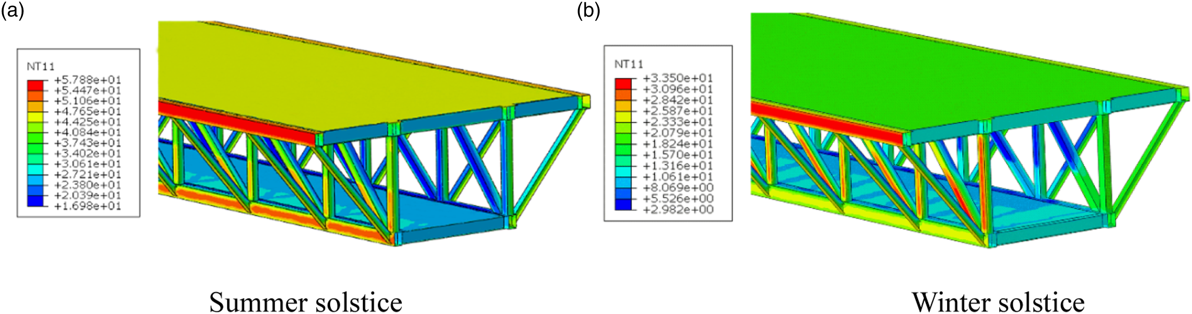

Vertical temperature gradient of the girder

The vertical temperature gradient of the steel truss girder on the summer solstice is shown in Figure 11(a). Every moment, there was a significant temperature difference at the junction of the side girder and the web members, with a maximum temperature difference of 15.4°C at 9:30. This condition was attributed to the direct shining on the east side of the side girder, while the end of the web member was entirely in shadow. From 8:30 to 10:30, the upper deck covered the upper part of the web members, resulting in a significant temperature difference. The maximum temperature difference occurred at 8:30, at 8.1 m from the upper deck. Meanwhile, the temperature of the web member decreased from 41.8°C to 34.2°C, and the sheltering effect caused the maximum transient temperature difference of the same member to reach 7.6°C. Thus, the sheltering effect of the upper deck had a significant impact on the structural temperature field and cannot be ignored.

Figure 11.

Vertical temperature gradient of the steel truss girder: (a) 1 day on June 22, 2022; (b) largest temperature gradient.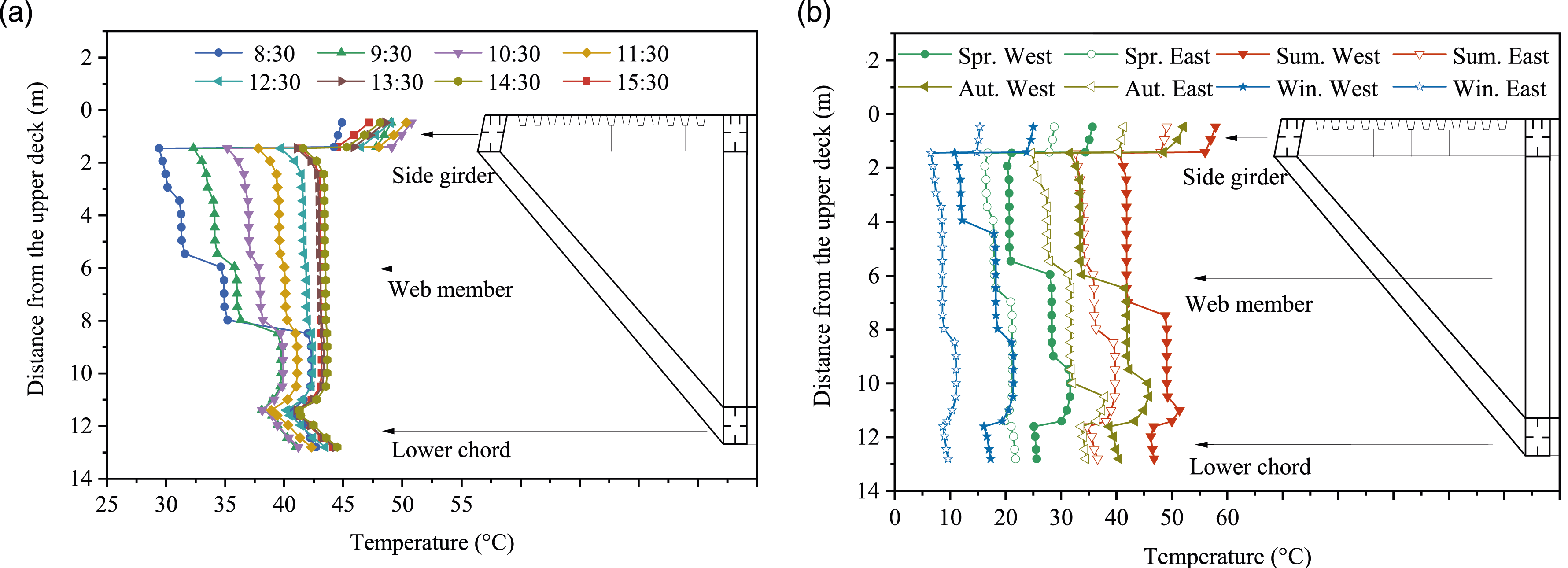

The most adverse vertical temperature gradient of the steel truss girder in four seasons is plotted in Figure 11(b). The vertical temperature difference on the west side was more prominent than on the east, because of the higher air temperature when the sun shines directly on the west side girder. In summer, the maximum temperature difference on the west side was 17.3°C. In winter, the maximum temperature difference on the east side was 8.8°C.

Transverse gradient of the girder

The transverse temperature gradient of the upper deck was uniform under the sunlight, but the lower deck was different. The reason was that the upper deck and web members surrounded the lower deck. For convenient representation, the middle position of the lower deck was positioned at coordinate 0, with the farthest coordinates on the east and west sides being −7m and 7m, as given in Figure 12.

Figure 12.

Transverse temperature gradient of the steel truss girder.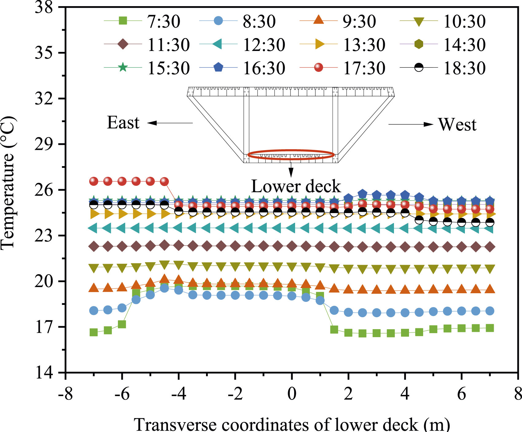

From 7:30 to 8:30, there was a significant temperature difference of 2.8°C at the transverse coordinates of −5.5 m and 1.5 m. The lower deck within the transverse coordinates of 1.5 m to 7m and −7.5 m to 5.5 m was obstructed by the upper deck and web members, whereas the range of −5.5 m to 1.5 m was not obstructed, resulting in a significant temperature difference at the junction. At other times, the temperature distribution was even because the lower deck was entirely in shadow.

Transverse difference of the girder

The research reported in the existed reference had revealed that for similar steel truss cable-stayed bridges with two-layer decks, the transverse temperature difference of the lower chords significantly impacted the horizontal rotation angle (Wang and Ding, 2019). Therefore, it was necessary to study the variation of the transverse temperature difference of the lower chords. It should be said that the transverse temperature difference in this simulation refers to the difference between the lower chords on the east and west side.

As is demonstrated in Figure 13 (a), the variation pattern of the transverse temperature difference in different seasons is similar. Before sunrise, the temperature difference was almost 0. The temperature difference gradually increased as the sun rose and shined directly on the eastern lower chord. At noon, both sides of the lower chord were exposed to the same solar radiation, and the temperature difference fell to 0. The sun continued to move to the west side, and the temperature difference grew again.

Figure 13.

Transverse temperature difference of the lower chord: (a) different seasons; (b) different orientations.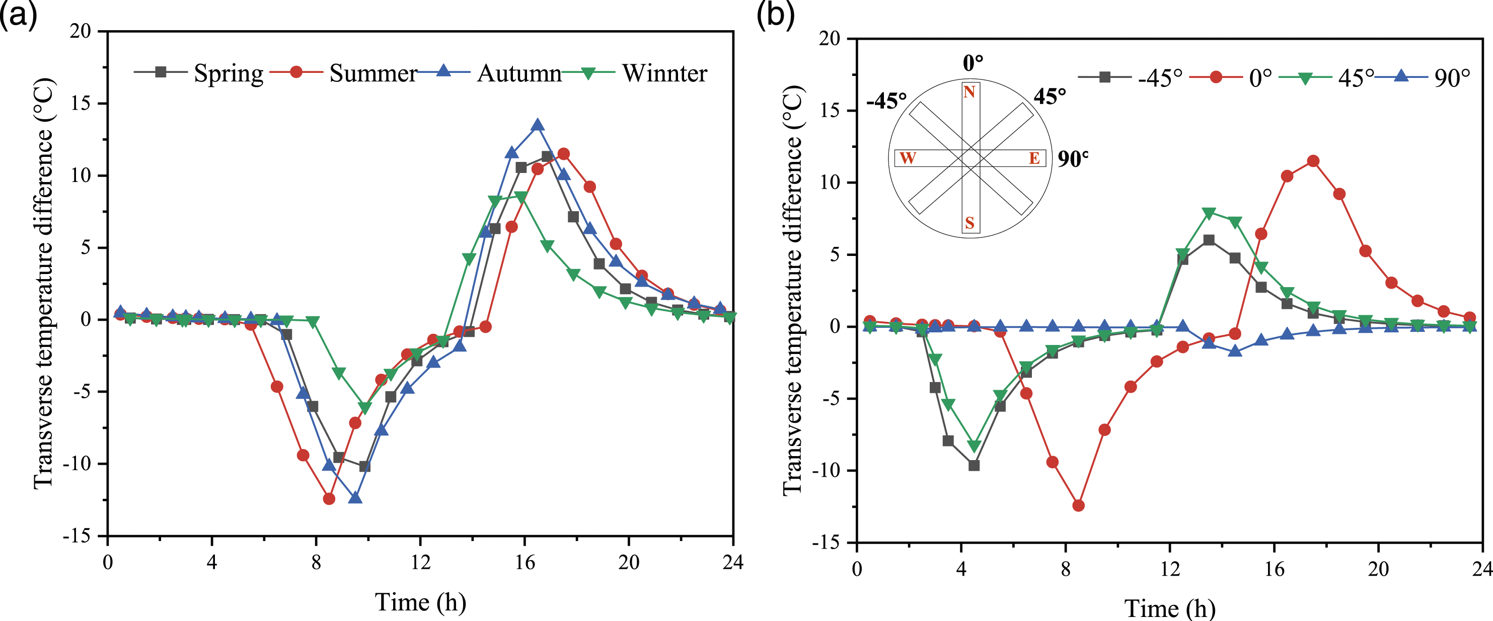

The influence of bridge direction (azimuth) on the transverse temperature difference of the lower chord was studied based on the steel truss girder. As shown in Figure 13 (b), four typical directions were selected, namely −45°, 0°, 45°, and 90°, all in summer. When the azimuth was 0°, the temperature difference was the largest, 13.1°C. As the azimuth of the bridge increased to 90°, the maximum temperature difference declined to 1.76°C. This can be attributed to the inability of direct solar radiation to reach the lower chord on both sides. As a consequence, the direction of the bridge has a considerable effect on the maximum temperature difference.

Thermal deformation of steel truss girder during construction stage

The maximum cantilever stage is one of the most adverse construction stages before the bridge closure. After being affected by sunlight, the plane bending deformation of the steel truss beam is large. This section studied the vertical, transverse, and longitudinal thermal deformations of the upper chord (M₂ and M₃), side girder (M₁ and M₄), and lower chord (M₅ and M₆) during this stage through thermo-mechanical coupling. The specific location is given in Figure 14.

Figure 14.

Location of M₁–M₆: (a) longitudinal view of maximum single cantilever stage; (b) cross-section 1-1.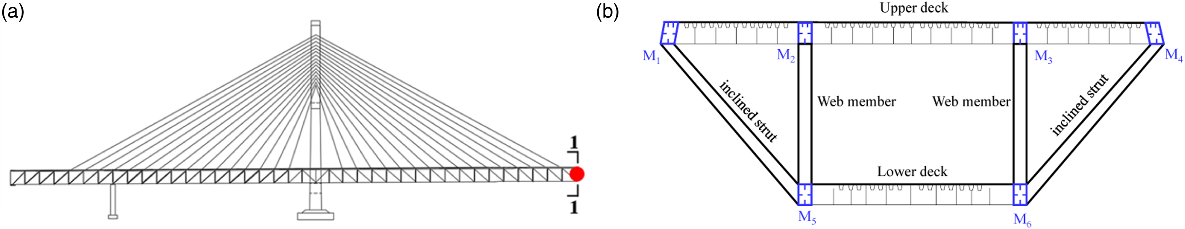

For cables, the cross-section is so small that the cable temperature is uniform. Zhu and Meng (2017) found that compared to the vertical temperature gradient inside the beam, the effect of temperature changes inside the steel cable on deflection was more significant. Therefore, this section considered that the temperature inside the cable varied sinusoidal, and there was a lag time between its extreme and the air temperature (Cao et al., 2011).

Vertical deformation of the girder

On the summer solstice and winter solstice, the real-time vertical deformation of members M₁–M₆ is shown in the Figure 15. As the sun rose, the temperature of the cable and the vertical temperature difference of the steel truss girder continued to increase. Under the combined effect, each member's downward vertical deformation varied greatly. At midday, the change in vertical deformation of the members was small, because of the decreasing vertical temperature difference (Figure 11). On the summer solstice, the maximum vertical deformation occurs at the upper chord M₂, which is 7.2 cm. On the winter solstice, the maximum vertical deformation of the upper chord M₂ was 5.1 cm.

Figure 15.

Vertical deformation of members: (a) summer solstice; (b) winter solstice.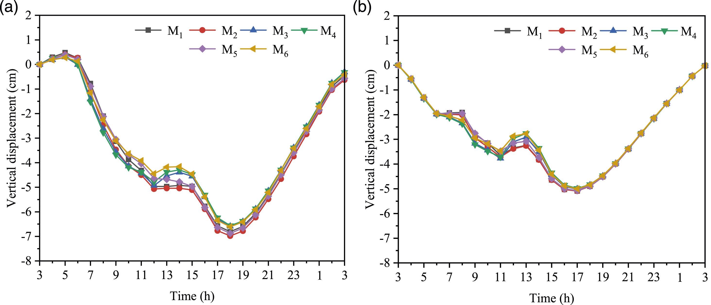

Longitudinal deformation of the girder

The longitudinal deformation of the girder in the real-time temperature field is presented in Figure 16. In the morning, the longitudinal deformation of the east side members M₁–M₂ was larger; In the afternoon, the value of the west side members M₃–M₄ was larger. Moreover, the deformation of members M₅–M₆ was generally smaller than that of members M₁–M_4. This can be attributed to the sheltering effect of the upper structure on the lower structure, resulting in low temperature of M₅–M_6. In Figure 16(a), at 15:00 on the summer solstice, the deformation of the side girder M₄ reached the maximum value of 6.4 cm among all members, while that of the lower chord M₅ was 4.7 cm. The difference in deformation between members M₄ and M₅ was 1.7 cm. In Figure 16(b), during a day in winter, the maximum longitudinal deformation of the side girder M₄ was 4.2 cm, and the maximum difference between the members was 1.3 cm.

Figure 16.

Longitudinal deformation of members: (a) summer solstice; (b) winter solstice.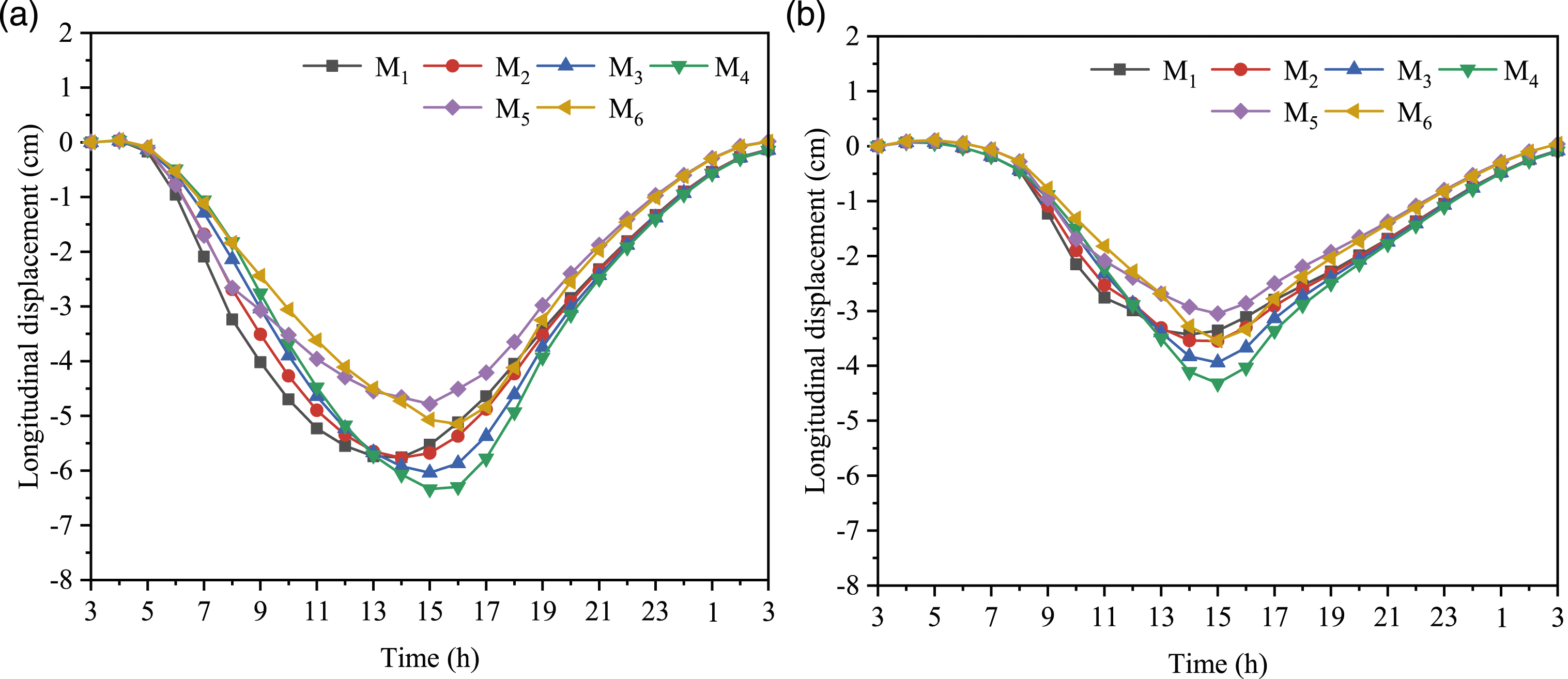

Transverse deformation of the girder

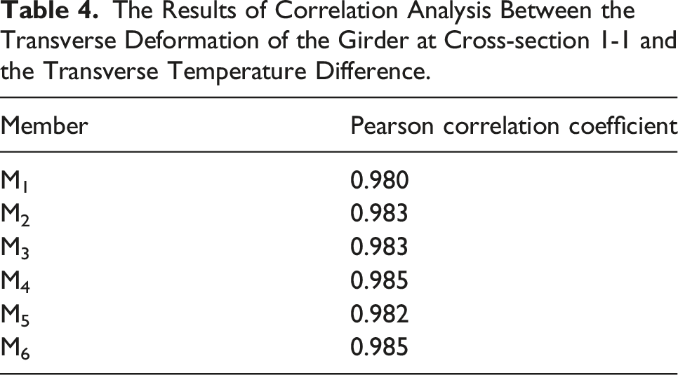
The variation of the transverse deformation of the girder on the summer solstice and winter solstice is given in Figure 17. The overall deformation trend of members M₁–M₆ was the same, with little change at night and intense change at daytime. On the summer solstice, the maximum deformation during the day reached 5.9 cm; On the winter solstice, the maximum deformation was 3.9 cm. By comparing the transverse temperature difference of the lower chord calculated in Figure 13 (a), it was found that the variation between the transverse deformation and the transverse temperature difference was consistent, and they almost reached their maximum and minimum values simultaneously.

Figure 17.

Transverse deformation of members: (a) summer solstice; (b) winter solstice.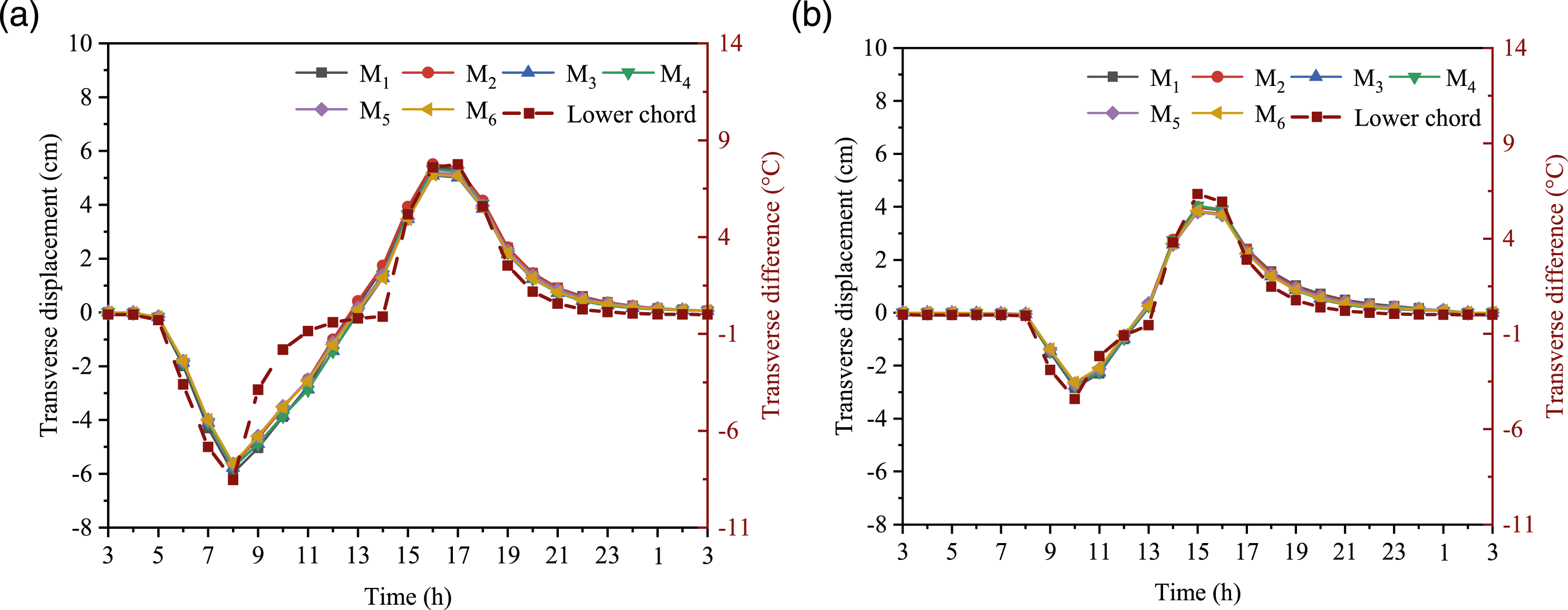

Table 4 shows the Pearson correlation analysis (Zhou et al., 2016a) between the transverse deformation of the girder at cross-section 1-1 and the transverse temperature difference. A generally strong positive correlation between the transverse deformation of the members M₁–M₆ and the transverse temperature difference of the lower chord can be observed. Therefore, it was reasonable to believe that the transverse temperature difference of the lower chord was the main factor controlling the transverse deformation of the girder during the construction stage.

Table 4.

The Results of Correlation Analysis Between the Transverse Deformation of the Girder at Cross-section 1-1 and the Transverse Temperature Difference.

Member	Pearson correlation coefficient
M₁	0.980
M₂	0.983
M₃	0.983
M₄	0.985
M₅	0.982
M₆	0.985

Conclusions

By considering geo-meteorological factors and the sheltering relationships, a temperature field analysis algorithm was developed, accurately simulating the temperature field and thermal deformation of the bridge during construction. The main conclusions of this study can be summarized as follows:

(1) By comparing with experimental data, the accuracy of the method for analyzing the sunlight temperature field of the steel truss cable-stayed bridge with two-layer decks was verified.

(2) Due to the obstruction of the upper structure, apparent shadow areas appeared at the web members and lower deck, causing a maximum temperature difference of 7.6°C in the bridge structure. It can be found that sheltering effect of the upper structure has a significant impact on the temperature field, which cannot be ignored.

(3) Study on the transverse temperature difference of the lower deck shows that the maximum transverse temperature difference of this north-south oriented bridge can reach 13.1°C, which is much larger than that of the same type of east-west oriented bridge, which is 1.8°C; and the comparison of transverse temperature difference and transverse deformation of different seasons reveals that the transverse temperature difference of the lower chord is the main factor controlling the transverse deformation of the steel truss girder during the construction stage.

(4) Sunlight has a large impact on the deformation of steel truss girder during construction. On the summer solstice, the maximum vertical, longitudinal, and transverse deformations of the main members are 7.2 cm, 6.4 cm, and 5.9 cm, respectively.

Footnotes

Declaration of conflicting interests

The author(s) declared no potential conflicts of interest with respect to the research, authorship, and/or publication of this article.

Funding

The author(s) disclosed receipt of the following financial support for the research, authorship, and/or publication of this article: This work was supported by the National Natural Science Foundation of China (Grant No. 52078333).

ORCID iD

Jinsong Zhu

References

Cao

Yim

Zhao

, et al. (2011) Temperature effects on cable stayed bridge using health monitoring system: a case study. Structural Health Monitoring 10(5): 523–537.

Catbas

Susoy

Frangopol

(2008) Structural health monitoring and reliability estimation: long span truss bridge application with environmental monitoring data. Engineering Structures 30(9): 2347–2359.

Chang

(2000) Thermal behavior of composite box-girder bridges. Structures and Buildings 140(2): 117–126.

Chen

(2008) Effects of Thermal Loads on Texas Steel Bridges. Austin, TX: The University of Texas at Austin.

Ding

Zhou

, et al. (2012) Thermal field characteristic analysis of steel box girder based on long-term measurement data. International Journal of Steel Structures 12(2): 219–232.

Emanual

Hulsey

(1978) Temperature distributions in composite bridges. Journal of the Structural Division 104(1): 65–78.

Fan

Liu

, et al. (2022) An efficient model for simulation of temperature field of steel–concrete composite beam bridges. Structures 43: 1868–1880.

Kehlbeck

(1981) Effect of Solar Radiation on the Bridge Structure. Beijing, China: China Railway Press. (in Chinese).

Kim

Park

, et al. (2015) Temperature variation in steel box girders of cable-stayed bridges during construction. Journal of Constructional Steel Research 112: 80–92.

10.

Lee

Kalkan

(2012) Analysis of thermal environmental effects on precast, prestressed concrete bridge girders: temperature differentials and thermal deformations. Advances in Structural Engineering 15(3): 447–459.

11.

(1996) Solar Physics. Beijing, China: Capital Normal University Press. (in Chinese).

12.

(2017) Study on Thermal Expansion Coefficient of Cable and Structural Performance of Prestressed Steel Structure under Temperature Action. Tianjin, China: Tianjin University. (in Chinese).

13.

Chen

Zhou

, et al. (2023) Thermal behaviors of bridges – a literature review. Advances in Structural Engineering 26(6): 985–1010.

14.

Lienhard

(2003) A Heat Transfer Textbook. 3rd edn. Cambridge, MA: Phlogiston Press.

15.

Liu

Qian

(2016) Thermal field characteristic analysis of steel bridge deck during high-temperature asphalt pavement paving. KSCE Journal of Civil Engineering 20(7): 2811–2821.

16.

Liu

Zhang

(2019) Review on solar thermal actions of bridge structures. China Civil Engineering Journal 52(5): 59–78. (in Chinese).

17.

Meng

(2019) Simulation and Prediction of Long-Term Deformation of Prestressed Concrete Bridges under Environmental Thermal and Vehicle Loads. Tianjin, China: Tianjin University. (in Chinese).

18.

Moorty

Roeder

(1992) Temperature-dependent bridge movements. Journal of Structural Engineering 118(4): 1090–1105.

19.

Priestley

MJN

(1976) Design temperature gradients for concrete bridges. New Zealand Engineering 31(9): 213–219.

20.

Roberts-Wollman

Breen

Cawrse

(2002) Measurements of thermal gradients and their effects on segmental concrete bridge. Journal of Bridge Engineering 7(3): 166–174.

21.

Roeder

(2003) Proposed design method for thermal bridge movements. Journal of Bridge Engineering 8(1): 12–19.

22.

Shan

Xia

, et al. (2023) Temperature behavior of cable-stayed bridges. Part I — global 3D temperature distribution by integrating heat-transfer analysis and field monitoring data. Advances in Structural Engineering 26(9): 1579–1599.

23.

Tong

Tham

FTK

(2001) Numerical modelling for temperature distribution in steel bridges. Computers & Structures 79(6): 583–593.

24.

Wang

Ding

(2019) Long-Term Monitoring of temperature effect on horizontal rotation angle at beam ends of a railway steel truss bridge. Journal of Bridge Engineering 24(10): 05019012.

25.

Wang

Fan

, et al. (2017) Thermal effects on curved steel box girder bridges and their countermeasures. Journal of Performance of Constructed Facilities 31(2): 04016091.

26.

Wang

Zhou

Ding

, et al. (2021) Long-Term monitoring of the temperature differences in a steel truss bridge with two-layer decks compared with bridge codes: case Study. Journal of Bridge Engineering 26(3): 05020013.

27.

Xia

Chen

Weng

, et al. (2012) Temperature effect on vibration properties of civil structures: a review and case studies. Journal of Civil Structural Health Monitoring 2(1): 29–46.

28.

Xia

Chen

Zhou

, et al. (2013) Field monitoring and numerical analysis of Tsing Ma Suspension Bridge temperature behavior. Structural Control and Health Monitoring 20(4): 560–575.

29.

Xia

Zhang

Tian

, et al. (2017) Experimental study of thermal effects on a long-span suspension bridge. Journal of Bridge Engineering 22(7): 04017034.

30.

Chen

, et al. (2010) Monitoring temperature effect on a long suspension bridge. Structural Control and Health Monitoring 17(6): 632–653.

31.

Yin

Zhao

(2014) Computer program for directed structure topology optimization. Chinese Journal of Applied Mechanics 31(6): 939–944. (in Chinese).

32.

Zhou

(2013) Thermal load in large-scale bridges: a state-of-the-art review. International Journal of Distributed Sensor Networks 9(12): 217983.

33.

Zhou

Deng

Xia

, et al. (2016a) A new sampling method in particle filter based on Pearson correlation coefficient. Neurocomputing 216: 208–215.

34.

Zhou

Xia

Brownjohn

, et al. (2016b) Temperature analysis of a long-span suspension bridge based on field monitoring and numerical simulation. Journal of Bridge Engineering 21(1): 04015027.

35.

Zhu

Meng

(2017) Effective and fine analysis for temperature effect of bridges in natural environments. Journal of Bridge Engineering 22(6): 1–19.

36.

Zhu

Sun

Guo

, et al. (2023) Fine analysis for non-uniform temperature field and effect of railway truss suspension bridge under solar radiation. Journal of Constructional Steel Research 210: 108098.

Thermal effect analysis of a steel truss cable-stayed bridge with two-layer decks under sunlight

Abstract

Keywords

Introduction

Thermal analysis method for bridge structures

Thermal environment of steel truss

Heat-Transfer Analysis

Heat-Transfer theory

Thermal Boundary Conditions

Direct solar radiation

Diffuse solar radiation

Reflected solar radiation

Atmospheric radiation

Surface environmental radiation

Diffuse surface radiation

Three-dimensional ray sheltering theory

Initial temperature filed

Numerical analysis and validation

Numerical analysis process

Validation

Case

Description of experimental bridge

Finite element simulation

Temperature distribution characteristics of the steel truss girder

Vertical temperature gradient of the girder

Transverse gradient of the girder

Transverse difference of the girder

Thermal deformation of steel truss girder during construction stage

Vertical deformation of the girder

Longitudinal deformation of the girder

Transverse deformation of the girder

Conclusions

Footnotes

Declaration of conflicting interests

Funding

ORCID iD

References