
Abstract
This study investigates four different joints under fluctuating tension cycles in the low-cycle fatigue (LCF) regime. The selected material was S960 ultra-high-strength steel, manufactured via the direct-quenching manufacturing route. Based on typical engineering solutions, the following joints were chosen to be investigated in the experimental tests: metal active gas and laser welded butt joints, fillet-welded load-carrying cruciform joints, and non-load-carrying double-sided transverse attachment joints. To evaluate the improvement gained by the post-weld treatment, both as-welded condition and high-frequency mechanical impact treated joints from all joint types were tested. In addition to the experimental tests, some of the joints were analyzed using finite element (FE) models, with the aim of comparing the accuracy of the different fatigue assessment methods and the effect of the toe radius on the computational fatigue lives. The results obtained from the experimental tests and FE analyses were compared with each other and with IIW recommendations using the nominal stress, structural hot-spot (HS) stress, effective notch stress (ENS) and 4R methods. Based on the results, the structural HS and 4R methods are very suitable for the fatigue strength assessment in the LCF regime. With the nominal stress method, the computational fatigue lives remained uniformly conservative, while with the ENS method, the results varied depending on the calculation method. Using the value r = 1 mm as the weld toe rounding is justified in the FE analysis.
Introduction
It is widely acknowledged that carbon dioxide emissions have an impact on global climate change, and that these emissions should be globally minimized as soon as possible. In the steel industry, with a global CO2 emissions share of about 6%, this challenge has been approached by developing a new nearly fossil-free steel production method, which applies electricity and hydrogen in steelmaking instead of coal and coke (Müller et al., 2021). However, it is currently expensive to produce steel using this method, and the costs are not expected to reach the level of those for steel produced via conventional manufacturing until 5–10 years from now (Pimm et al., 2021). Hence, and to minimize emissions and the amount of steel produced in the future, the design of efficient structures made of appropriate fossil-free steel will create the basis of eco-friendly and economically viable products and solutions.
Nowadays, high-strength steels (HSSs) and ultra-high-strength steels (UHSS) are commonly used in steel structures. The potential for lightweight structures, good manufacturability, and high load-bearing capacity support the use of these materials. In addition, the abovementioned characteristics can reduce the amount of CO2 emissions, for example, by reducing the dry weight, increasing the load-carrying capacity, and optimizing the amount of steel used, thereby complementing the comprehensive reduction of CO2 emissions begun by switching to fossil-free steel. However, new solutions and steel grades create new challenges and demands for design and manufacturing. Good material properties and manufacturability do not automatically mean a good end product, and therefore the behavior of structures and structural components in connection with various load situations must be known. For example, the IIW recommendations for estimating fatigue resistance and effect of residual stresses (RS) (Hobbacher, 2016; Marquis and Barsoum, 2016) are applicable to yield strengths of up to f y = 960 MPa. UHSSs usually suffer from the sharp notches and, consequently, the applications of post-weld treatments (PWT) are of paramount importance to enhance fatigue strength capacity (Zhao et al., 2014: 64). Also, the recommendations are often limited to the high-cycle fatigue (HFC) regime, where external loads do not cause stresses close to the yielding strength and the crack growth occurs as an elastic phenomenon. In low-cycle fatigue (LCF) regime, however, stresses are higher and material response is macroscopically plastic in every cycle (Schijve, 2009: 161–162, 168.).
In this study, SSAB Strenx 960 steel plate with a plate thickness of 8 mm was studied in the LCF regime under a constant amplitude load. The research was performed by testing four different joints, namely laser and metal active gas (MAG)-welded butt joints, fillet-welded load-carrying cruciform (LC-X) joints, and non-load-carrying double-sided transverse attachment (NLC-X) joints, all in both as-welded (AW) and post-treated conditions. Post-weld treatment was performed with high-frequency mechanical impact (HFMI) treatment. By locally plasticizing the material, the treatment affects the weld toe geometry, material microstructure and residual stresses (Aldén et al., 2020: 1948). Roughly 700 MPa nominal stress variation and R = 0.1 stress ratio were applied.
The results of the experimental tests were analyzed by applying the nominal stress, structural hot-spot (HS) stress, and effective notch stress (ENS) methods. The results were calculated fatigue (FAT) classes, and comparisons between the experimental and computational fatigue lives as well as the IIW recommendations were made. In addition to the ENS method, the results of finite element (FE) analysis were used for the fatigue life predictions in the HS and 4R methods. The computational fatigue lives were compared to the results of the experimental tests; in addition, the effect of the toe radius on the accuracy of the ENS and 4R methods was investigated by performing the FE analysis with four different toe radii.
Materials and methods
Base material and welding consumables
The studied base material was SSAB Strenx 960 steel plate with a plate thickness of 8 mm Mechanical properties of the plate are given in Table 1. The studied UHSS grade was a low-alloyed steel manufactured via the direct quenching (DQ) manufacturing route. DQ, with the chemical composition given in Table 2, forms a bainitic and martensitic microstructure for the base material with a grain size of about 1 μm, providing high strength. The steel can be classified as dual-phase or ultra-fine-grain steel, but also as complex-phase steel due to the various bainite phases. The DQ production method also ensured a low carbon content, which together with the low extent of alloying, produced a low-carbon equivalent. Thus, the probability of the cold cracking of welds was diminished and the preheating only required thick plates.
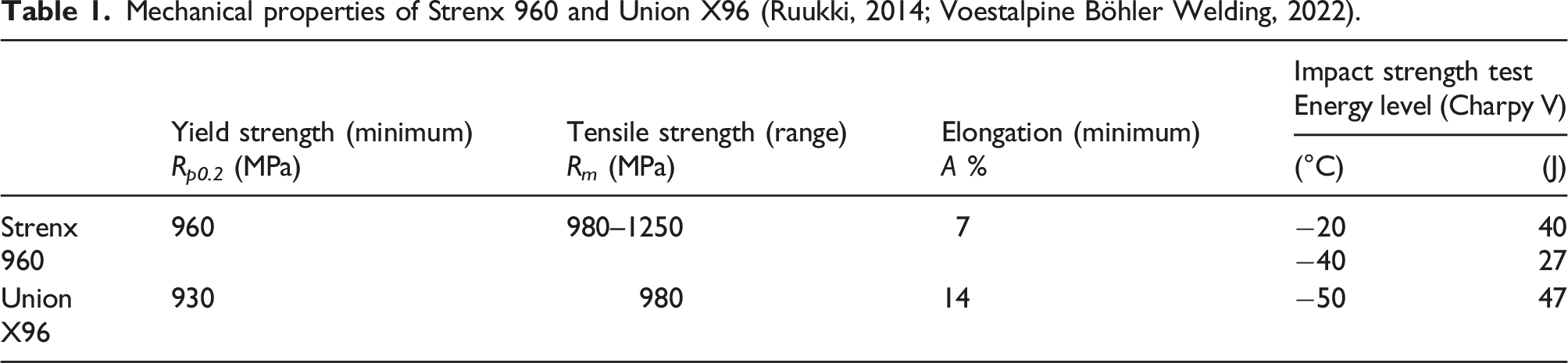
Mechanical properties of Strenx 960 and Union X96 (Ruukki, 2014; Voestalpine Böhler Welding, 2022).
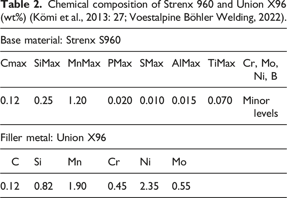
Chemical composition of Strenx 960 and Union X96 (wt%) (Kömi et al., 2013: 27; Voestalpine Böhler Welding, 2022).
Due to the welding, the softening of DQ S960 MC, with a bainitic-martensitic microstructure, is typically slightly greater than with quenched and tempered UHSSs; however, a hard and non-tempered martensitic microstructure is not formed because of low alloying. Thus, the 800–500°C cooling time (t8/5) of less than 4 s could be considered in the case of equal strength joints, when a t8/5 of less than 15 s is otherwise acceptable. Although the joint is said to achieve equal strength, softening is always found at the local stage heat affected zone (HAZ), and thus there are lower strength zones that are generated by phase transitions, carbide spheroidization and tempering. Therefore, in general, methods that minimize and focus the heat input are widely used.
The used fillet metal was Böhler Welding Union X96 solid wire, which is classified as strength-matching with the base material. Woikoski SK-10 (Ag+10% CO2) was used as a shielding gas. To the authors’ knowledge, small amounts of CO2 are known to stabilize the arc, improve the weld geometry, and reduce spatter and slag.
Test specimens
The studied specimen types were chosen based on the representative welded components typically found in engineering structures, and thus four different joints were selected. These were metal active gas (MAG)-welded butt joints, laser-welded butt joints, fillet-welded load-carrying cruciform (LC-X) joints, and non-load-carrying double-sided transverse attachment (cruciform, NLC-X) joints. To evaluate the improvement gained by post-weld treatment (PWT), high-frequency mechanical impact (HFMI) treatment was applied using a commercial Pfeifer Dynatec HiFIT device with a hammer pin radius of 2.5 mm. Two test specimens in each series (joint type and condition) were fatigue-tested, for a total number of 16 specimens.
The shape and dimensions of the dual symmetric test specimens (without the transverse reinforcement plates) are shown in Figure 1. The purpose of the widenings at the joint area was to ensure that the weld run-on and run-off were outside the tested area, and thus ensure uniform joint geometry over the joint area after the widenings were removed. Shape of the pre-cut sheet for the manufacture of welded joints.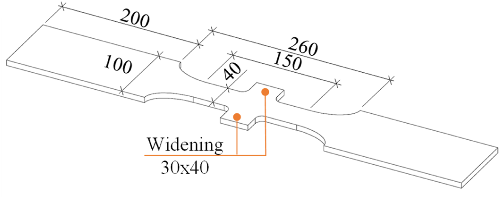
Tack welding was performed with tungsten inert gas (TIG) from both ends of the groove. Robotized MAG welding was done using a Motoman EA1900 N welding robot, a Kemppi Pro 4200 Evolution power source, and a ProMig 520R MXE control unit. The butt welds were performed with two passes in the x-groove in the flat (PA) position. The wire was aligned in the center of the joint, applying a working angle of 90° and a 5° pushing travel angle. The X-joints were made with fillet welds in the horizontal–vertical (PB) position, with the wire aligned about 1 mm on the side of the lower plate and applying a working angle of 45° and an 18° pushing travel angle. Each specimen was tilted to produce a 4° downhill angle to obtain a better weld geometry compared to the horizontal alignment. All specimens were allowed to cool to room temperature between passes.
Manufacturer’s recommended and calculated values for welding energy EW and cooling time t8/5.
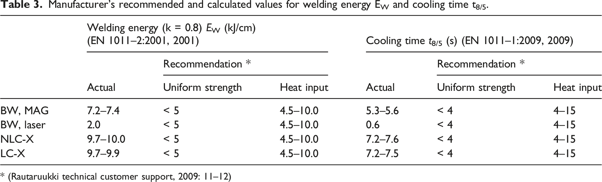
* (Rautaruukki technical customer support, 2009: 11–12)
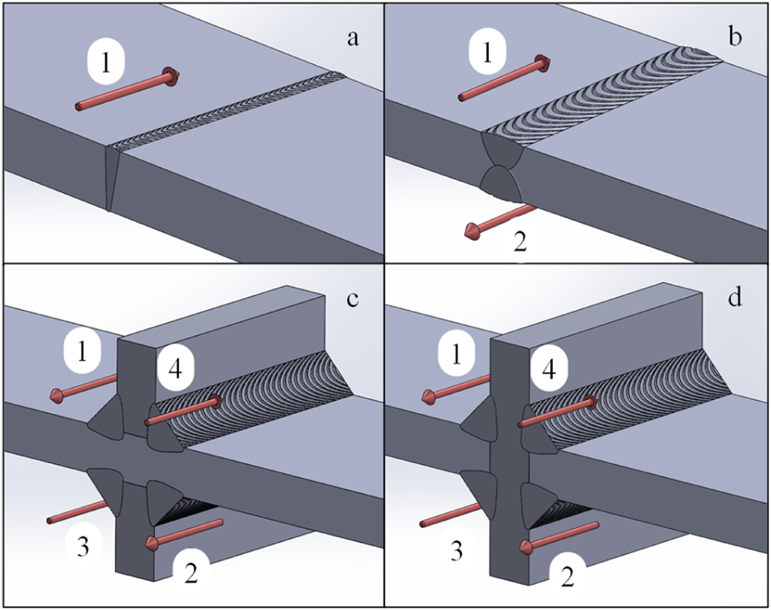
Welding sequence of the (a) laser-welded butt weld, (b) MAG-welded butt weld, (c) MAG-welded non-load-carrying double-sided transverse attachment, and (d) MAG-filled-welded load-carrying cruciform joint.
Pre-test measurements
In the selected specimens, as representative specimens in each specimen category, pre-test measurements were carried out before the fatigue testing to obtain the information required in the tests and to collect data for the post-analysis of the test results. The applied tests were hardness tests, surface shape measurements and residual stress measurements. The purpose of the hardness measurements was to identify changes in the material properties at the HAZ. In particular, the areas close to the potential crack nucleation were measured to identify any reduction in the material strength due to the welding as well as the widths of the different sub-zones. In addition, the geometries of the joints’ cross-sections were visually observed from the macro graphs. Based on the hardness measurements, a 50 to 60 HV decrease in material hardness in the fine-grained area near the surface was perceptible, indicating about 900 MPa ultimate strength (Rm) (see Figure 3). Compared to the reported ultimate strength of the base material equal to 980–1250 MPa, the difference is considerable. Hardness distribution of a non-load-carrying double-sided transverse attachment joint (JR3B1).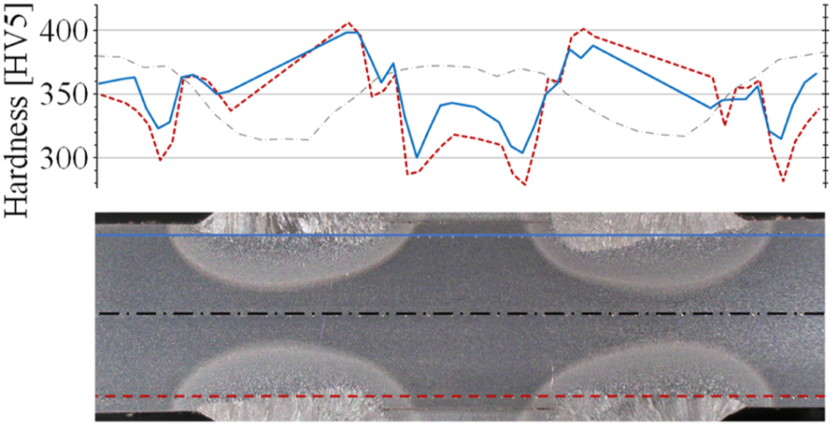
The residual stresses of each different specimen were measured with X-ray diffraction. Eight measurement points were located, with the first one at the weld toe and the last one 10 mm from the weld toe, as shown in Figure 4. Based on the measurements, the residual stresses at the weld toe line varied from 100 MPa in tension to 500 MPa in compression. In this regard, it is also worth mentioning that the welding preparation was conducted while preventing welding deformation; as a result, small or even compressive residual stresses were measured from the joints in the AW condition. In all studied specimen types, residual stress levels changed sign and were in compression after HFMI treatment, being between 450 and 800 MPa in compression at the weld toe. The effect of the HFMI treatment on the residual stresses was identified at a distance of about 3 mm from weld toe at the shortest, but at the load-carrying X-joints (LCX-joint) and laser-welded butt joints, the effect was noticed even at a distance of up to 6 mm and 10 mm, respectively. Residual stress distribution of a non-load-carrying double-sided transverse attachment joint (JR3B1) in the AW and HFMI treated conditions.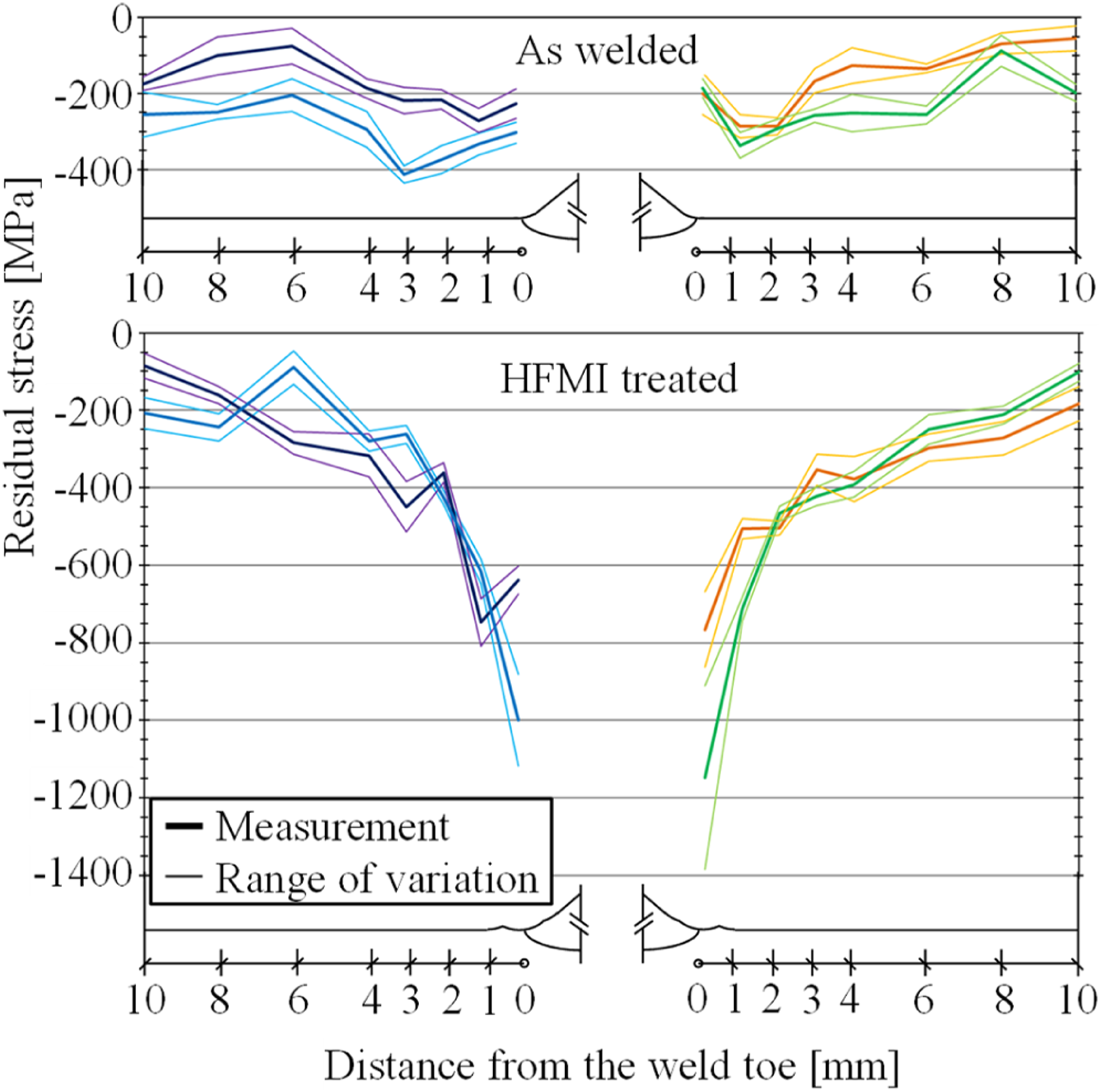
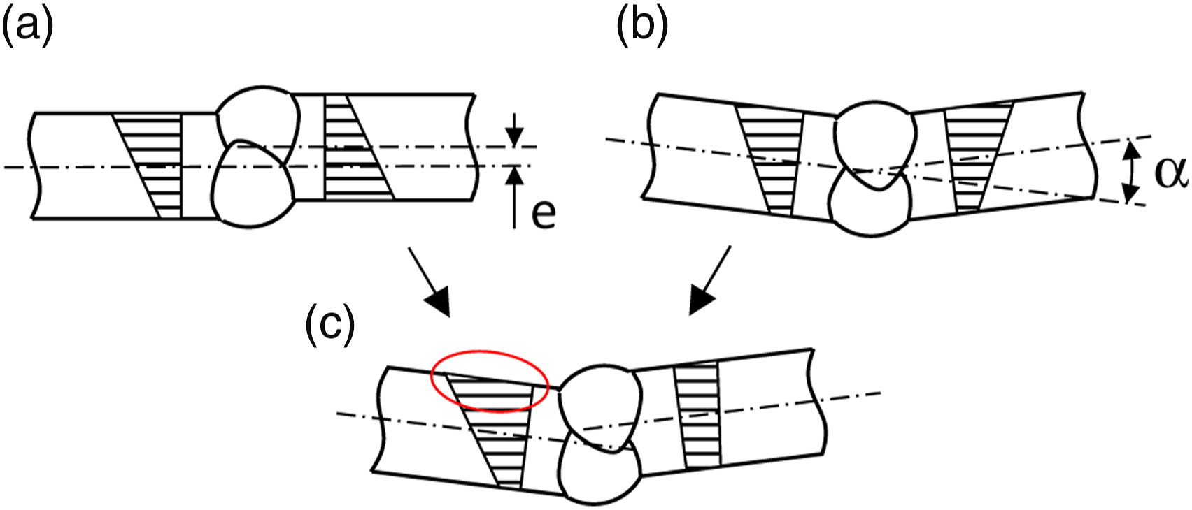
Angular and axial misalignment together with weld notch angles.
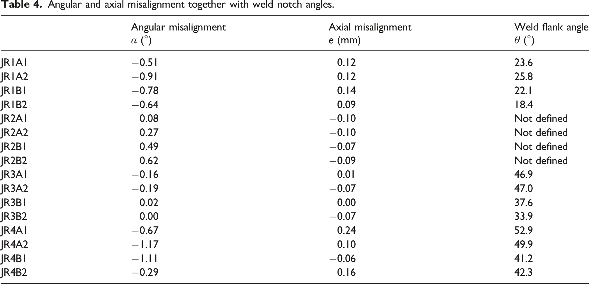
Misalignment may consist of angle or axial misalignment or both, as shown in Figure 5. The stress magnification factors Km,e and Km,α could be calculated by means of formulas obtained from the literature, but in the combination of cases, the interaction was obtained from equation (1). Due to the rigid attachment of the clamps, the ends were assumed to be fully restrained (λ = 3). (Hobbacher, 2016: 127.) Structural stress over thickness: (a) axial, (b) angular, (c) axial and angular misalignment.
Fatigue testing
Fatigue tests were performed in the LUT Laboratory of Steel Structures at room temperature, utilizing a 400 kN servo-hydraulic test rig. The load was created by moving the upper clamp axially with servo-hydraulic actuators using constant amplitude uniaxial loading. Both the upper and lower clamps were located on the same axis, so by placing the specimens perpendicular between them, the external load consisted of only pure tension. During the test, the minimum and maximum of the applied load, displacement, and strain values for a certain cycle and time were periodically measured. The values of the load and displacement were read directly from the control unit of the test rig. The values of the strain were determined from the center line of the specimen using one strain gauge at a distance of 0.4 t (3.2 mm) from the weld toe. The side of the gauge was defined on the side where crack was predicted to nucleate based on maximum stress magnification factor from equation (1) and visual inspection.
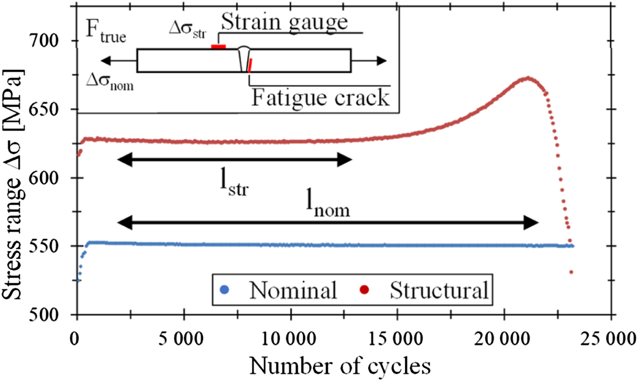
All tests were started by loading the test specimens quasistatically at the maximum tension so that the permanent strain caused by the hysteresis could be noted and removed from the cyclic measurement sequence. After that, the specimens were loaded dynamically between the minimum and maximum stresses, using load cycles with a 1–2 Hz frequency. The magnitude of secondary stress was determined in each specimen on the basis of a strain gauge by applying equation (2). After the dynamic test had reached the required stress levels, the test was continued by keeping the strain constant. For this reason, the structural stress results correspond approximately to the stress range based on the measured strain, and the nominal stress had to be calculated by using the measured force and the cross-sectional area as shown in equation (3). An example of the measured nominal stress (applied force) and structural stress (strain gauge measurements) during the fatigue test is shown in Figure 6. At the beginning of both curves, it is noticeable that the power levels are rising to the required levels during the first tens of cycles. In addition, the increase in structural stress as the test progresses indicated the crack growth from a different side to the gauge. Nominal and structural stress range during the test (JR2B2, gauge side 2A).
Finite element analysis
The FE analyses were performed by applying the HS and ENS methods. FE models were created based on the surface measurement data to minimize geometrical errors. No factors other than shape were taken into account in the FE analyses, and the material was thought to be homogeneous and linear-elastic (Young’s modulus of E = 210 GPa and Poisson’s ratio of v = 0.3) without residual stresses, as per the HS stress and ENS methods. Considering the above as well as the applied assessment methods, the joints in the AW condition were only assumed to produce comparable results. However, based on the visual inspection of the surface measurement data, the BW and NLC-X joints in the HFMI-treated condition also needed to be analyzed. Modelling and post-processing were performed with the Siemens FEMAP 2020.2 software using an NX Nastran solver.
Model generation
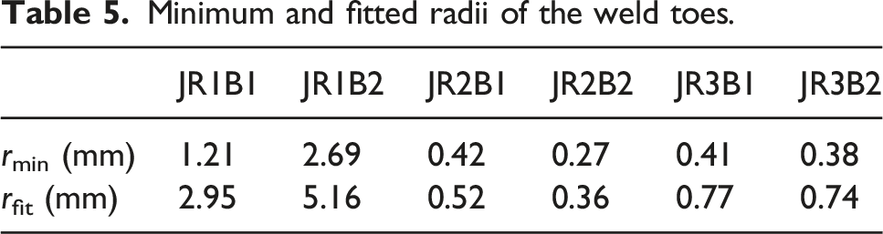
Minimum and fitted radii of the weld toes.
Meshing
The analysis of the models was performed with quadratic (Q8) isoparametric plane strain elements with a thickness of 1 mm. The ENS method element size was determined by the size of the radius of the weld toe under consideration. Following the IIW recommendations (Hobbacher, 2016: 29), the element size was in all cases limited to ¼ of the defined minimum radius. However, the maximum size length of the elements was limited to 0.1 mm, since some sharp forms were always noticed next to the radius, that may have otherwise been ignored. Around the areas to be analyzed, a regular quadrilateral element shape was applied, and the elements were regularly increased, as presented in Figure 7. An example of the meshing of a weld toe. Element size at the radius 0.07 x 0.07 mm.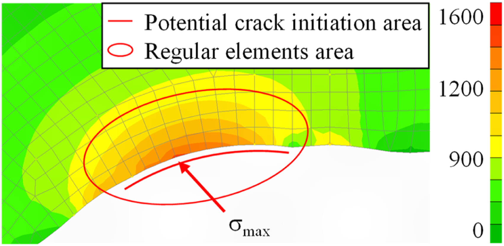
In the HS stress method, IIW recommends that the element size be below or equal to 4/10 of the sheet thickness (Hobbacher, 2016: 24). Thus, an element size of about 3.2 mm would have been enough in all cases. However, the models were made with the same element size as in the ENS method to consider the effect of the true shape of the weld toe line.
Load and boundary conditions
The load and boundary conditions were transferred to the model through rigid elements, created at both ends. The created rigid elements allowed the nodes to move in the direction of the plane thickness, but in the perpendicular direction, the nodes were kept in a straight line. Thus, transformation under the load was possible, but rotation occurred as a solid plane. The load was introduced uniformly over the thickness, only at one end. The used magnitude of the loads was the nominal stress range, given in Appendix A1. The direction of the force was always the direction of the x-axis. With the boundary conditions, shown in Figure 8, it was ensured that no shear or bending stress was generated in the model. Principle drawing load and boundary conditions of the models.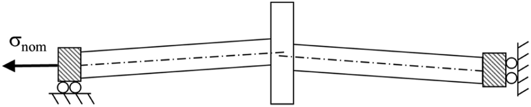
Fatigue assessment using the 4R method
To consider and understand the essential fatigue parameters, the 4R method was applied to the MAG-welded butt joints and NLC-X joints. The 4 R method is a notch stress-based approach method developed by Nykänen and Björk in the early 2010s, and it can be applied to welded joints and cut edges. The method simulates the material’s cyclic behavior, considering four important material and joint parameters: material ultimate strength (R m ), applied stress ratio (R), residual stress (σ res ), and rounding of the weld toe (rtrue). Of course, since the material’s local elastic-plastic material model with the kinematic hardening rule is considered, the material parameters for the Ramberg–Osgood equation, for example, must be known. (Björk et al., 2018)
In the 4R method, the ENS approach is used to calculate the local notch stress range Δσ
k
, but the reference notch stress range Δσ
k,ref
, applied in fatigue calculations, is calculated by applying the local stress ratio R
local
(the ratio of the local minimum and maximum stresses) equation (4).
Results
The results of the fatigue tests were compared using three different stress-based approaches, namely nominal stress, structural HS stress and ENS. The nominal and structural stress levels were determined based on Equation (3) and Equation (2), respectively. However, since crack initiation did not always start from the side of the strain gauge, particularly in the case of low angular misalignment, structural stress was transferred to the correct weld toe line by applying the stress magnification factor K m , given in equation (1). It should be noted that the maximum stress was not always on this side. Based on the nominal and structural stresses, the HS stress concentration factor k hs could be calculated by applying equation (6).
The notch stress ranges were determined based on the FE calculations. For the specimens in the AW condition, the ENS was calculated by applying a toe radius of 1 mm and, in the HFMI-treated specimens, by applying the measured true toe radii. In the case of the PWT laser-welded BW and LC-X joints, the stresses were not specified. The fatigue notch factor K
f
was calculated using equation (7) and the ENS concentration factor K
w
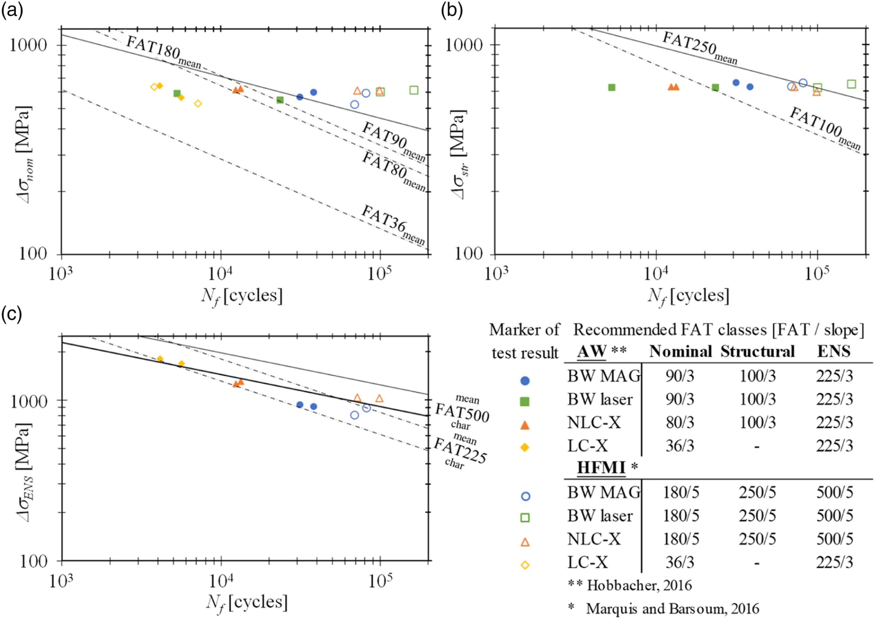
using equation (8). All the results, categorized by each applied method, are shown as S–N graphs in Figure 9 and tabulated in Appendix A1. Fatigue test results in an S–N graph, based on the (a) nominal stress, (b) structural HS stress, and (c) ENS stress methods.
Nominal stress method
The results based on the nominal stress ranges are presented in Figure 9(a). FAT36 (mean fatigue strength approximately 49 MPa with jσ = 1.37) (Radaj et al., 2006: 20) is generally applied for the LC-X joints (root failure) (Hobbacher, 2016: 45), and the obtained test results are clearly above this with a calculated FAT59 (FAT50% = 81 MPa; henceforth, mean fatigue strength is presented in parenthesis). The results are well in line with the slope parameter of m = 3. For butt joints, instead, FAT90 (123) is recommended (Hobbacher, 2016: 44), and one laser-welded specimen with a fatigue strength of FAT60 (82) did not reach this recommendation. A second specimen, with FAT91 (125), was in agreement with the recommended value, but still clearly below the MAG-welded butt joints with an average value of FAT110 (151). For the NLC-X joints, FAT80 (110) is recommended (Hobbacher, 2016: 53), which is in line with the average FAT84 (115).
Excluding the LC-X joint failing from the weld root, the effect of HFMI treatment is clearly noticeable. With m = 3, the MAG-welded BW obtained FAT137 (187), the laser-welded BW FAT178 (244) and the NLC-X joint FAT155 (212). Respectively, with m = 5, FAT212 (290), FAT257 (352), and FAT236 (323) were achieved. IIW allows the fatigue limit to be increased 1.5 times with the slope parameter of m = 3 (Hobbacher, 2016: 71) or the value FAT47(180) with m = 5 (Marquis and Barsoum, 2016: 23). In all cases, the test results were above these limits.
Structural hot-spot stress method
The results based on the structural stress range are presented in Figure 9(b). All joints suitable for the HS method had a recommended fatigue class of FAT100 (137) (Hobbacher, 2016: 61). The reference value was only achieved with the MAG-welded BW specimen, with an average FAT124 (170). The results also fit well on the slope parameter of m = 3. For the laser-welded BW, only one exceeded the recommendation with FAT104 (142), and the other fell below, with FAT63 (87). Neither of the NLC-X joints achieved the recommendation but remained on average at FAT85 (117).
For the HFMI-treated joints, FAT250 (343) with a slope parameter of m = 5 is recommended by IIW (Marquis and Barsoum, 2016: 26). All PWT joints were well compliant with the recommendation, obtaining values of MAG-welded BW: FAT250 (343), laser welded BW: 274 (376) and NLC-X joint: FAT238 (327). Meanwhile, the other recommendation of FAT140 (192) with a slope parameter of m = 3 (Hobbacher, 2016: 70) seems conservative, with the joints obtaining values of FAT162 (221), FAT191 (261), and FAT156 (214), respectively.
Effective notch stress method
The results based on the ENS ranges are presented in Figure 9(c). For the ENS method, IIW recommends the characteristic curve FAT225 for joints in the AW condition with a slope parameter of m = 3 (Hobbacher, 2016: 62) and, after HFMI treatment, FAT500 with m = 5 (Marquis and Barsoum, 2016: 27). All joints in the AW condition were above the recommendation, with FAT238 (173); however, they remained clearly below the mean curve of FAT309 (225). As expected with the HFMI treatment, the fatigue strength appeared to rise, but only came close to the characteristic curve by an average of FAT362(496) with a slope parameter of m = 5. However, with m = 3, FAT236 (323) was achieved.
Discussion
Computational fatigue lives
In addition to the S–N curves presented in results, the nominal, structural HS and ENS methods (appendix A.1) were used to determine the computational fatigue lives of the specimens. The IIW recommended fatigue classes, summarized in Figure 9, were used in the calculations. The results based on the mean and characteristic curves are shown in Figure 10 as a comparison of the experimental (Nf,exp) and computational (Nf,comp) fatigue lives. Comparison of the experimental (Nf,exp) and computational (Nf,comp) fatigue lives based on the mean and characteristic curves; (a) nominal stress, (b) structural HS stress and (c) ENS methods.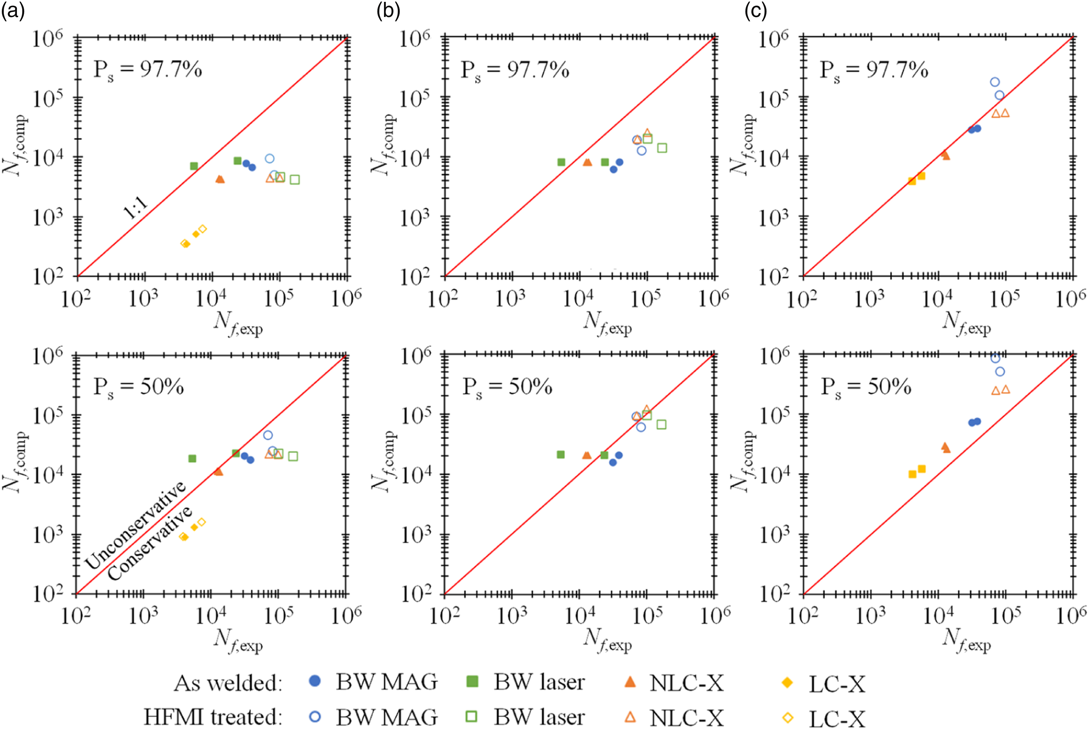
In the structural HS method, all computational fatigue lives are well aligned with the test results. The only clear exception is one laser-welded butt joint, for which a lower fatigue life is clearly visible in the experimental test, as well as in the nominal stress results. The higher fatigue class given by the HFMI treatment (FAT250 (343) with a slope parameter of m = 5) can be considered well justified, although the given minimum structural HS stress concentration value is not exceeded (Marquis and Barsoum, 2016: 26).
With the previously mentioned exception, the calculated fatigue lives of the nominal stress method remain on the conservative side, predicting shorter service lives than those obtained from the tests. The results for the HFMI-treated specimens are slightly more conservative than for the specimens in the AW condition; consequently, the fatigue class could be even higher than recommended in the design standards. Meanwhile, the ENS method provides unconservative results. Excluding the HFMI-treated MAG-welded butt joint, the computational fatigue lives lead to an almost characteristic curve. The abovementioned MAG-welded butt joint even exceeds the characteristic curve and thus clearly differs from the line of the other results. The large deviation can be explained by the low ENS concentration factor K W . According to the recommendations, the stress concentration factor should be at least 1.6, yet it is only about 1.3 for this joint (Marquis and Barsoum, 2016: 27). By applying structural HS stress Δσ str, fix and the factor K W = 1.6, the recalculated service lives decrease to become well in line with the other results.
Fatigue lives calculated using the hot-spot and 4R methods
The HS and 4R methods were used to estimate the fatigue life of the MAG-welded BW and NLC-X joints. The methods utilized the stresses obtained from the FE analysis. In the HS method, FAT100 with a slope of three and FAT250 with a slope of five were used for the AW and HFMI-treated joints, respectively. The calculations for the 4R method were performed with the values given in chapter 2.6 and using ENS stresses with a toe radius of r = 1 mm. The results of the calculations are shown in Figure 11. Comparison of the experimental (Nf,exp) and computational (Nf,comp) fatigue lives based on the mean and characteristic curves; (a) structural HS stress and (b) 4R methods.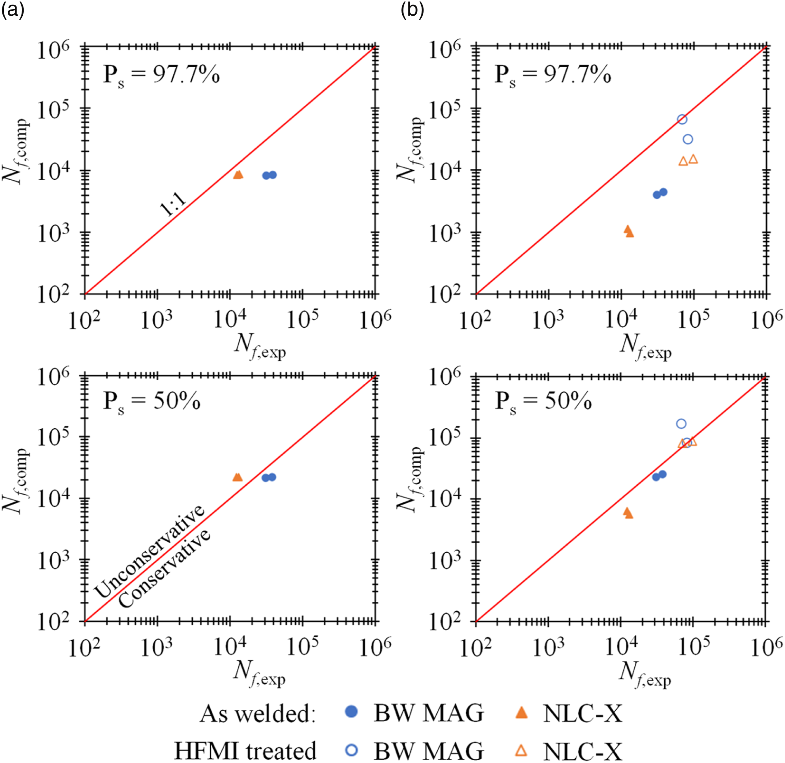
Based on the results, the fatigue lives estimated using both methods correspond well to the results of the experimental tests. The results with the HS method can be stated to be at least as accurate, and even slightly more in line with the test results, than the results measured with the strain gauge (Figure 10(b)). With the 4R method, the results are very much in line with the test results, and in terms of accuracy are comparable to the results of the ENS method (Figure 10(c)). However, the results are fundamentally more conservative than with the ENS method, even leading to conservative fatigue life estimations in the AW condition joints. For joints treated with HFMI, the results are even more accurate than using the ENS method, corresponding well to the fatigue test results.
Fatigue strength of the HFMI-treated specimens
For comparison, the computational service lives of the HFMI-treated specimens were estimated in two ways, namely using the recommendations of Hobbacher (2016) and Marquis and Barsoum (2016). Subsequently, by comparing the computational and experimental fatigue lives, it was possible to evaluate the representativeness of the increased fatigue class for the PWT joints. The calculations were made using the FAT categories given in Section 3 and Figure 9. The results based on the mean and characteristic curves are shown in Figure 12 as a comparison of the experimental (Nf,exp) and computational (Nf,comp) fatigue lives. Comparison of the HFMI-treated specimens’ experimental (Nf,exp) and computational (Nf,comp) fatigue lives based on the mean and characteristic curves; (a) nominal stress, (b) structural HS stress and (c) ENS methods.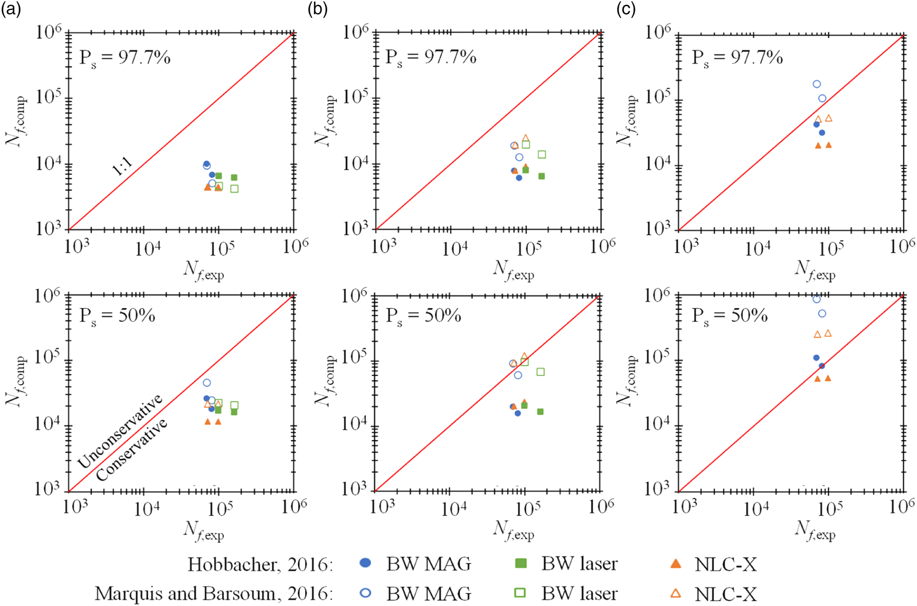
With the nominal stress method, the computational fatigue lives obtained with both recommendations are very similar. From the point of view of dimensioning, it does not matter which one is used. However, when using the HS and ENS methods, the results clearly differ between the recommendations. In the HS method, Marquis et al. recommend the fatigue class FAT 180 (247) with a slope parameter of m = 5, which gives well-aligned results and thus their use in the dimensioning is justified. Hobbacher instead recommends fatigue class FAT140 (192) with m = 3, which gives results that are clearly on the safe side. In the ENS method again, the computational fatigue lives based on Hobbacher’s recommendations of FAT225 (309) with m = 3 match the results of the experimental tests. The results obtained with Marquis et al.’s recommendations, i.e. FAT500 (686) with m = 5, are clearly unconservative, giving results close to the design curve.
Effect of the toe radii on the results of the ENS and 4R methods
In the FE calculations of the MAG-welded butt joints and NLC-X joints in the AW condition, the rounding of the weld toe was simulated in four different ways: fitted curve (r = rtrue), fitted arc (r = rfit), 1 mm root radius (r = 1 mm), and true radius plus 1 mm radius (r = rtrue + 1 mm). The stresses given by the models were used in the calculations of the ENS and 4R methods, and the obtained computational fatigue lives were compared with the results of the experimental tests. In the ENS method, FAT225 (309) with a slope parameter of m = 3 was used. In the 4R method, the assessments were made as described in Section 2.6, using the characteristic reference curve Cref, char = 1020.83 with m = 5.85. A comparison of the results using the ENS concept and the 4R method is presented in Figure 13. Effect of the weld toe radii on the relationship between the computational and experimental service lives. MAG-welded BW and NLC-X joints in the AW condition were included in the comparison.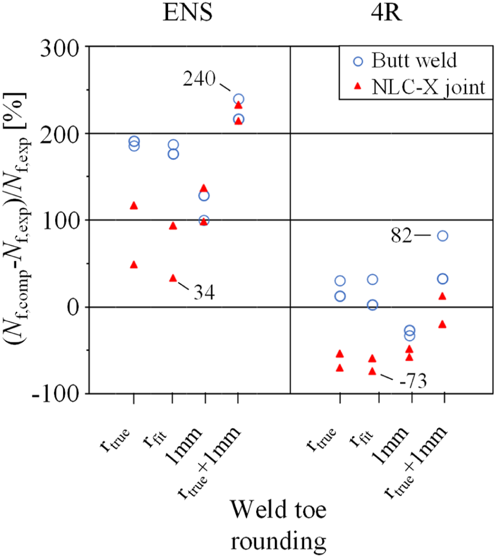
The comparison shows that the computational lives calculated by the ENS method are all on the conservative side, while the 4R method provides both conservative and unconservative results depending on the applied toe radius. By applying r = rtrue or r = rfit, the results are very scattered in both methods; however, it should be considered that the ENS method gives a maximum difference of almost 191%, while the 4R method gives a maximum difference of 73%. In addition, in the case of the NLC-X joints, the variation between the results is clearly greater in the ENS concept than in the 4R method, while in the butt joints the difference is the other way around, albeit smaller. Considerably smaller variations, with a maximum difference of 39%, were obtained by applying r = 1 mm and r = rtrue + 1 mm with the ENS method and r = 1 mm with the 4R method. The most accurate computational fatigue live predictions were obtained with the 4R method, the difference being only 41% lower on average. Even though the variation was small with the ENS method, the predicted service lives were far from the experimental test results, being 116% and 226% higher on average. By applying the 4R method and r = rtrue + 1 mm, the results for the NLC-X joints were the most accurate among the tested specimens. However, the results for the butt joints turned out to be more accurate with all other weld toe rounding applied in the 4R method.
For comparison, the HFMI-treated MAG-welded butt joint and NLC-X joints were also subjected to FE analysis, applying a fitted surface shape, and the ENS and 4R methods were used to predict the fatigue lives, as described above. Based on the results (Figure 14), the predicted fatigue lives of the butt joints showed a large, almost 200% deviation in both methods, but with the 4R method the results were closer to the results of the experimental tests. In the NLC-X joints, the variation was lower with both methods than with the butt joints. However, with the ENS method the results were further from the results of the experimental tests than they were with the 4R method. For the NLC-X joints, the variation was reduced, but the accuracy was maintained, when using the ENS method. With the 4R method, the variation decreased clearly, and the estimated fatigue lives had a maximum 15% difference from the results of the experimental tests. Effect of assessment method on the relationship between the computational and experimental service lives. MAG-welded BW and NLC-X joints in the HFMI-treated condition and with a fitted surface model were included in the comparison.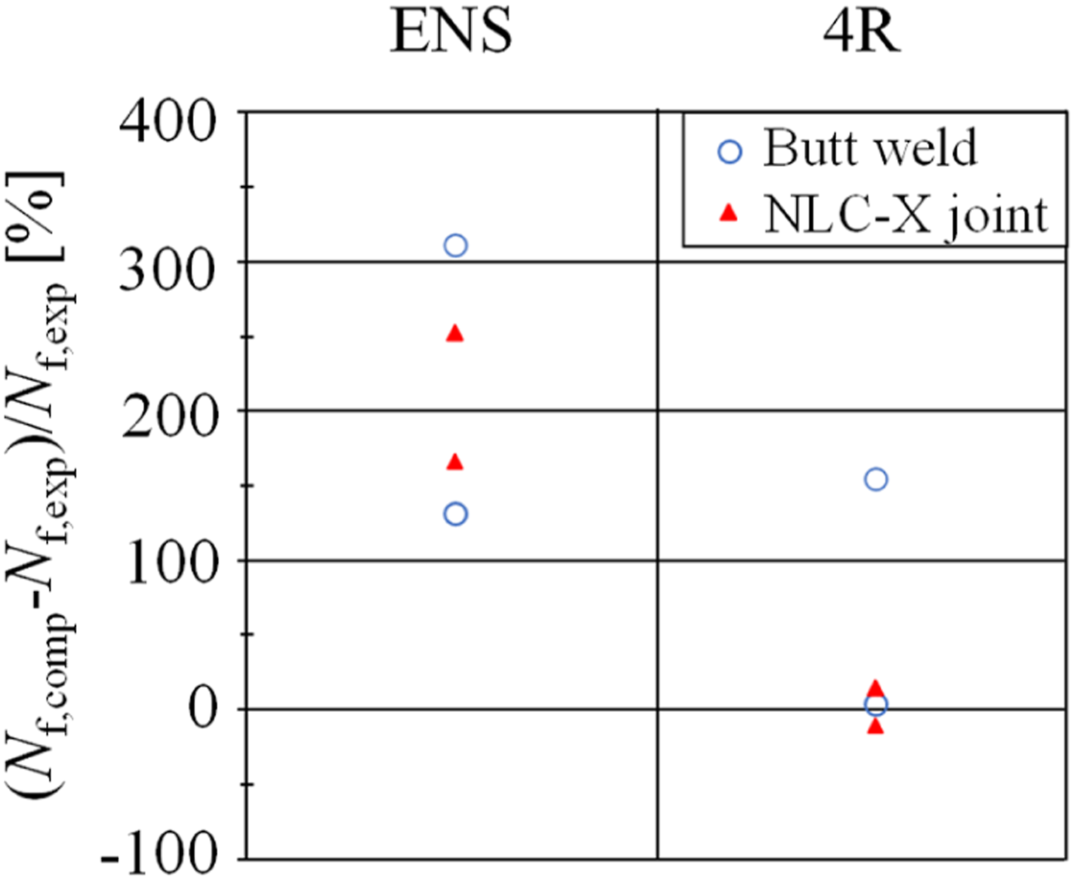
Conclusions
In this paper, experimental and numerical analyses were carried out to investigate four different joints, made by Strenx S960 structural steel, under fluctuating tension cycles in the LCF regime. Half of the test specimens underwent PWT to evaluate the effect of HFMI treatment on fatigue strength. The results obtained from the experimental tests were compared to the IIW recommendations and to the computational fatigue lives obtained from the nominal stress, structural HS stress, ENS, and 4R methods. Based on the evaluations and experimental study, the following conclusions can be drawn: • Based on the values measured from the experimental tests, the nominal stress method gives slightly conservative results, while the results from the structural HS method are well in line with the recommendations. • FE analysis, using the weld toe rounding r = 1 mm in the AW condition, showed that the computational fatigue lives of the structural HS method are in accordance with the recommendations. However, the ENS method provides uniformly unconservative computational fatigue lives, while they are slightly conservative with the 4R method. For the HFMI-treated specimens, and using the weld toe rounding r = rfit, the 4R method provides fatigue life predictions that are well in line with the recommendations, but the computational fatigue lives with the ENS method are clearly too large compared to the experimental results. In the case of the MAG-welded BW, the big difference is partly explained by the small KW factor. • As the weld toe is critical for crack initiation, HFMI treatment could improve the fatigue strength of the experimentally tested joints. It is possible to calculate the computational fatigue life of HFMI-treated specimens according to two different recommendations: Hobbacher (2016) and Marquis and Barsoum (2016). The fatigue lives obtained by the nominal stress method are uniformly on the conservative side, and which recommendation to use is not decisive for the results. With the structural HS method, FAT180 with a slope parameter of m = 5 gives clearly more accurate fatigue life estimates than FAT140 with m = 3. With the ENS method, using the fatigue class FAT225 with the slope parameter of m = 3, instead of the increased FAT500 with m = 5, is justified based on the results. • In both the ENS and 4R methods, the stress used in the calculations is obtained from the weld toe using FE analysis. For the joints in the AW condition, it is justified to use a weld toe rounding of r = 1 mm in both methods. However, the computational fatigue lives based on the ENS method differ from the experimental test results by more than +100%, while with the 4R method the difference is less than −60%. With the HFMI-treated specimens, using FE analysis with the measured surface model r = rfit, the 4R method provides very accurate fatigue life predictions, while with the ENS method, the dispersion between the variation is large and the difference from the experimental test results is more than +100%.
Footnotes
Declaration of conflicting interests
The author(s) declared no potential conflicts of interest with respect to the research, authorship and/or publication of this article.
Funding
The author(s) disclosed receipt of the following financial support for the research, authorship, and/or publication of this article: This work has been carried out in the Fossil-Free Steel Applications (FOSSA) project (Grant ID 5498/31/2021). The authors wish to thank Business Finland for the financial support.
Appendix
Fatigue test results.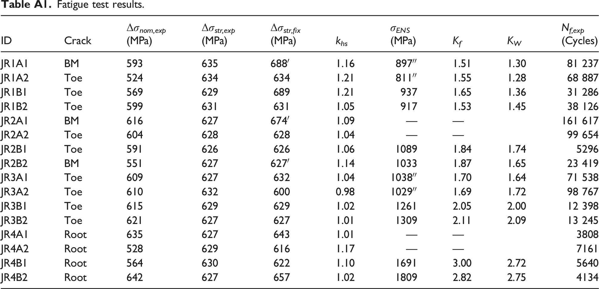
ID
Crack
Δσ
nom,exp
Δσ
str,exp
Δσ
str,fix
k
hs
σ
ENS
K
f
K
W
N
f,exp
(MPa)
(MPa)
(MPa)
(MPa)
(Cycles)
JR1A1
BM
593
635
688′
1.16
897″
1.51
1.30
81 237
JR1A2
Toe
524
634
634
1.21
811″
1.55
1.28
68 887
JR1B1
Toe
569
629
689
1.21
937
1.65
1.36
31 286
JR1B2
Toe
599
631
631
1.05
917
1.53
1.45
38 126
JR2A1
BM
616
627
674′
1.09
—
—
161 617
JR2A2
Toe
604
628
628
1.04
—
—
99 654
JR2B1
Toe
591
626
626
1.06
1089
1.84
1.74
5296
JR2B2
BM
551
627
627′
1.14
1033
1.87
1.65
23 419
JR3A1
Toe
609
627
632
1.04
1038″
1.70
1.64
71 538
JR3A2
Toe
610
632
600
0.98
1029″
1.69
1.72
98 767
JR3B1
Toe
615
629
629
1.02
1261
2.05
2.00
12 398
JR3B2
Toe
621
627
627
1.01
1309
2.11
2.09
13 245
JR4A1
Root
635
627
643
1.01
—
—
3808
JR4A2
Root
528
629
616
1.17
—
—
7161
JR4B1
Root
564
630
622
1.10
1691
3.00
2.72
5640
JR4B2
Root
642
627
657
1.02
1809
2.82
2.75
4134