
Abstract
The large amounts of hospitality and tourism-related search data sampled at different frequencies have long presented a challenge for hospitality and tourism demand forecasting. This study aims to evaluate the applicability of large panels of search series sampled at daily frequencies to improve the forecast precision of monthly hotel demand. In particular, a hybrid mixed-data sampling regression approach integrating a dynamic factor model and forecast combinations is the first reported method to incorporate mixed-frequency data while remaining parsimonious and flexible. A case study is undertaken by investigating Sanya, the southernmost city in Hainan province, as a tourist destination using 9 years of the experimental data set. Dynamic factor analysis is used to extract the information from large panels of web search series, and forecast combinations are attempted to obtain the final prediction results of the individual forecasts to enhance the prediction accuracy further. The empirical analysis results suggest that the developed hybrid forecast approach leads to improvements in monthly forecasts of hotel occupancy over its competitors.
Keywords
Introduction
Given the perishability of hospitality and tourism products, the real-time and accurate forecasting of hospitality and tourism demand is vital in revenue management to guide enterprises in long-term investment planning and strategic decisions (Chu, 2011; Li and Law 2020; Weatherford and Kimes, 2003). Inaccurate forecasts mislead them to make erroneous development plans and decisions, thus resulting in the unnecessary wastage of resources and even leading to the bankruptcy of the business (Norsworthy and Tsai, 1998). The high-frequency search data generated by Internet users can objectively reflect tourists’ attention and the potential hospitality and tourism demand, they can also help to enhance the forecast performance of the model (Yang et al., 2015; Zhang et al., 2020). However, the current prediction technology can only deal with the prediction task of the same frequency data, which, to a certain extent, limits the application of the model and the predictive capability (Kim and Swanson, 2017). Furthermore, when the web search data are used for prediction, a large number of key word explanatory variables bring new challenges to the model. This study addresses these two problems in the prediction of hotel demand.
With the comprehensive popularization of Internet technology, Internet information search is closely related to people’s daily lives and has become an important tool, particularly for tourists, to make decisions and conduct online transactions (Fesenmaier et al., 2009, 2010; TIA, 2008; Vila et al., 2018). The search record generated by Internet information exploration reflects the public opinions and attention of the tourists and essentially gives an early signal of tourist flow (Li and Law, 2020; Zhang et al., 2017). However, in practical applications, a dilemma usually faced by researchers is that the hospitality and tourism-related data are sampled at different frequencies. On the one hand, hospitality and tourism demand variables are generally monthly frequency data, while the online search data are generally daily or weekly high-frequency data containing potentially valuable feature information (Ghysels et al., 2007). On the other hand, researchers cannot directly incorporate mixed-frequency queries into a prediction model to forecast hospitality and tourism demand. High-frequency variables must be converted to low frequency by simple weighted average or summation method to meet the requirements of the consistent frequency of the variables in the current prediction technology, including time series models, econometric models, and artificial intelligence technologies. However, this solution may not be optimal, and it will lose potential useful information, thus resulting in progressively ineffective and inconsistent estimates and affecting the prediction accuracy (Andreou et al., 2010; Ghysels et al., 2007; Kim and Swanson, 2017; Owyang et al., 2010). Therefore, a forecasting scheme must be developed to enhance the predictability of the model. The mixed-data sampling (MIDAS) model developed by Ghysels et al. (2004) can solve the prediction problem of the data sampled at different frequencies. It allows the predicted variable to have different sampling frequencies, thereby avoiding the information loss caused by simple weighted average or summation scheme. This method has been widely used in the prediction of various macroeconomic indicators (Pan et al., 2018; Yuan and Lee, 2019).
The second challenge is incorporating large data sets into the MIDAS model while still being parsimonious. This incorporation involves the aggregation of multiple indicators and attracts the attention of academics (Brynjolfsson et al., 2016). Existing research mainly focuses on three methods to integrate web search data into the prediction model: first, by using statistical methods, such as Pearson correlation coefficient, to select key word variables with predictive ability and directly bringing the selected variables into the model (Choi and Varian, 2012; Zhang et al., 2017); second, by using a simple weighted average or summation, where multiple key word variables are aggregated into a comprehensive indicator (Yang et al., 2015); and third, by extracting the composite search index using factor analysis (Li et al., 2015).
Although these methods improve the prediction ability of the model under certain conditions, they are no longer suitable for a large number of key word variables. Directly bringing the key word series into the model likely results in numerous information duplication and overfitting problems (Varian, 2014), and the parameter proliferation problems caused by too many explanatory variables may be more evident (Owyang et al., 2010). The second method may lead to the information loss of key word variables and affect the prediction accuracy (Li et al., 2017). Factor analysis can extract common factors from large data sets (Stock and Watson, 2002). Using these factors can enhance the forecast precision of the model (Kim and Swanson, 2017). However, factor analysis mainly deals with sectional data, and the hospitality and tourism demand forecast uses time series in a large sample. In addition, the key assumption of the classical factor model is that the heterogeneity parts are orthogonal to one another, which means that all the correlations among the data are attributed to static common factors. Thus, the prediction results are not optimal. The dynamic factor model relaxes these assumptions, and it can extract information from high-dimensional time series data. Studies have shown that the introduction of dynamic factor models is conducive to the prediction of macroeconomic variables (Forni et al., 2003; Li et al., 2017). Forecast combinations can address structure breaks and model instability under certain circumstances (Timmermann, 2006). A large number of prior studies have shown that forecast combinations can improve prediction performance by using information from all models rather than relying on a single specific model (Aiolfi et al., 2010; Stock and Watson, 2004). Following the recent work by Andreou et al. (2013) and Gomez Zamudio and Ibarra (2017), and so on, this study introduces dynamic factor model and forecast combinations as two complementary approaches to deal with large-scale data that cannot be handled in one go.
The application of a large amount of hospitality and tourism-related search data sampled at different frequencies in demand forecasting needs further exploration. This study proposes a hybrid MIDAS approach integrating a dynamic factor model and forecast combinations to predict hotel occupancy. To evaluate the prediction power of the constructed approach, Sanya, a tourist city in China’s Hainan province, is used as an experimental case by collecting the key word variables related to the destination from January 2011 to December 2019. To ensure the parsimony of the model, the dynamic factor method is used to obtain the factor variables before forecasting, and each common factor is taken into the MIDAS model to predict the hotel occupancy. Then, the prediction results of the individual forecasts of the single-factor MIDAS model are combined to obtain the final predicted value. We conclude that the methodologies described herein can lead to improvements in prediction accuracy over its competitors.
The rest of the article is structured as follows: an extensive literature review is undertaken in the second section. Then, the conceptual analysis is presented in the third section. The fourth section constructs prediction methods used in this work. Next, the fifth section elaborates on the empirical analysis, results and discussion, and robustness check. Finally, the article concludes and offers a future course of action in this area.
Literature review
Hospitality and tourism demand forecasting
Various demand forecasting methods reported so far in hospitality and tourism mainly include time series models, econometric models, and artificial intelligence technologies (Song and Li, 2008; Song et al., 2019).
The time series methods represented by the autoregressive (AR) integrated moving average and the exponential smoothing model are used to predict demand based on the historical data derived from systematic observations (Chu, 2009; Guizzardi and Stacchini, 2015; Li et al., 2017; Song and Li, 2008; Stock and Watson, 2002). Econometric techniques, such as vector autoregression, construct models on the basis of statistical theory to detect the causal relationship between tourism demand variables and their influencing factors (Smeral, 2019; Song and Witt, 2006; Song and Li, 2008; Wong et al., 2007). Artificial intelligence methods include support vector regression (SVR), artificial neural network, deep learning method, and so on. These methods mainly model the nonlinear nature of tourism demand. The research results show that when the data possess nonlinear characteristics, artificial intelligent methods can effectively improve the model prediction capabilities compared with the benchmark models (Hassani et al., 2015; Law and Au, 1999; Law et al., 2019; Pai and Hong, 2005; Palmer et al., 2006; Zhang et al., 2020). However, no fixed prediction technology has excelled in all circumstances (Song and Li, 2008).
The aforementioned demand prediction models require that the predicted variables and the prediction variables have an equal sampling frequency, which, however, limits the application of the model to a certain extent and affects prediction accuracy (Kim and Swanson, 2017).
Forecasting with search engine data and dimension reduction
When consumers’ travel motivation is stimulated, tourists tend to explore and understand the related information of various holiday-making destinations to arrive at decisions (Gnoth, 1997; Uysal and Jurowski, 1994). With the popularity of the Internet, online information query has become an important and essential tool for consumer decision-making (Fesenmaier et al., 2009, 2010; Ho and Liu, 2005). Compared with traditional information search, web information search not only saves consumers’ time and cost but also provides more credible information (O’Connor, 1999). Moreover, information search behavior usually precedes tourism behavior (Pan et al., 2012). Tourist information search reveals different aspects of the travel process (Kim et al., 2007). These information searches are recorded by search engines, which objectively reflect the attention of the tourists. Therefore, key word variables can be used as the leading indicators of hospitality and tourism demand. Compared with statistical data, this kind of online search data is timely, easily accessible, and sensitive to tourists’ behavior. Many prior studies have reported in prediction research on social and economic activities based on the search engine data (Li et al., 2017).
In the field of hospitality and tourism, researchers mainly use Google and Baidu search queries to predict demand. To select effective key word variables for prediction, data dimensionality reduction methods mainly include using statistical techniques to filter key words, weighted sum scheme to aggregate key word variables into a comprehensive index, and factor analysis method (Choi and Varian, 2012; Li et al., 2017; Loureno et al., 2020; Yang et al., 2015; Zhang et al., 2017, 2019). The empirical outcomes suggest that the addition of search engine data can further enhance the forecast accuracy. For example, the ARMA with weekly Google trend data was used to forecast the monthly hotel room demand in Charleston City in the southeastern United States. In the empirical application, five key words are directly brought into the model for prediction, and the results indicate that the addition of Google data can improve the predictability of the model (Pan et al., 2012). For dimensionality reduction, Yang et al. (2015) transformed the key word variables into a composite index by a weighted average scheme and verified the cointegration relationship between the key word composite index and the tourist volume of China’s Hainan. Then, they incorporated the composite variable into the ARMA to predict Chinese tourist flow. Considering the nonlinear fluctuation characteristics of tourism demand, Zhang et al. (2017) used the Pearson cross-correlation analysis method to retain the four key word prediction variables with a higher correlation with the predicted variables. The selected variables were incorporated into the SVR algorithm to forecast the tourist flow of China. The results show that the addition of search data can enhance forecast power. Sun et al. (2019) constructed a single-layer artificial neural network algorithm and used Google and Baidu composite search index to forecast the tourist volume of Beijing; the composite index was constructed by a shift and sum approach. Other studies have also been reported to corroborate similar conclusions (Choi and Varian, 2012; Huang et al., 2017; Li et al., 2018; Park et al., 2016; Sun et al., 2020; Wei and Cui, 2018; Zhang et al., 2020). With the advance of academic research, online big data from multiple sources such as search engines and social media platforms are used to predict tourism demand (Li et al., 2020).
The existing literature mainly uses the time series model and artificial intelligence method when using high-frequency web online queries to forecast trends. However, none of these prediction techniques can directly model the mixed-frequency data set. The solution is to convert the high-frequency variable into a low-frequency one by a simple weighted average, thereby losing the characteristic information of high-frequency data (Ghysels et al., 2007; Owyang et al., 2010). In addition, the prediction accuracy will be affected by directly bringing the key word variables into the model and aggregating them into a comprehensive index (Li et al., 2017). Moreover, the classical factor model can show good dimensionality reduction ability in processing cross-sectional data. However, with the enlargement of time series, classic factor analysis is no longer the optimal scheme. The application of Internet search data in the hotel demand forecast needs further exploration. Furthermore, Baidu high-frequency web online data has not been applied in the hotel demand forecast, and the specific prediction effect needs to be tested.
Forecasting with MIDAS and forecast combinations
To avoid information loss caused by transforming mixed-frequency data into the same frequency by simple averaging and summing, the MIDAS regression developed by Ghysels et al. (2004) can be used to construct a forecasting technique with different frequencies while still being parsimonious. However, the MIDAS model was originally proposed for mixed-frequency data to forecast the volatility of the stock market (Ghysels et al., 2005; Leon et al., 2007). Later, the MIDAS and its variants have been successfully deployed in the field of macroeconomic forecasting (Li et al., 2015; Xu et al., 2020).
The application of MIDAS in hotel demand forecasting remains unexplored. Bangwayo-Skeete and Skeete (2015) directly introduced data from Google Trends into the MIDAS model to predict the tourist flows to five tourist destinations in the Caribbean. Meanwhile, Qin and Liu (2019) used weekly key word variables into the multivariate MIDAS approach to predict the tourist flows in China. Wen et al. (2020) proposed an improved MIDAS approach to forecast tourist volumes in Hong Kong from Mainland China with search index. The results suggest that the introduction of MIDAS can improve the forecasting accuracy of the model. Other similar studies have also been reported similar findings (Havranek and Zeynalov, 2019; Volchek et al., 2019; Wen et al., 2019).
Since the original study conducted by Bates and Granger (1969), forecast combinations have attracted extensive attention. This method combines the prediction results of individual models by using predetermined weighting schemes, thereby improving the forecasting performance over that offered by individual models (Gomez-Zamudio and Ibarra, 2017). Timmermann (2006) and Kim and Swanson (2014) have discussed this topic. Timmermann (2006) provided an excellent survey on forecast combinations. One of the justified reasons for using forecast combinations is that due to the various uncertainties in the modeling process, we regard the results of individual models as approximations, and we can combine the information sets of the prediction results of different models to generate a better prediction (Aastveit et al., 2014; Timmermann, 2006). A second reason is that forecast combinations can, to a certain extend, address the instability and structural mutation of the model under certain conditions, whereas a single model cannot (Stock and Watson, 2004). Moreover, a single model may suffer from an unknown form of error setting bias (Stock and Watson, 2004). A large and growing body of research shows that forecast combinations can improve prediction accuracy and robustness by using the information from all models rather than relying on a single specific model (Aiolfi et al., 2010; Timmermann, 2006). Forecast combinations have been widely used in the field of macroeconomic forecasting (Timmermann, 2006).
To address large panels of high-frequency data, Andreou et al. (2013) proposed two complementary prediction methods: (1) using data dimension reduction methods such as principal component analysis and factor analysis to extract a few common factors from a large number of time series and (2) combining the results of individual MIDAS models with a single factor, more accurate, and robust results are obtained. This approach has been applied to a large number of empirical studies. For example, to forecast Mexico’s GDP, Gomez Zamudio and Ibarra (2017) used factor analysis to extract a few common factors from 392 daily financial series and combined the forecast results of the single-factor MIDAS models with forecast combinations. The results show that this approach significantly improves prediction accuracy relative to the single-factor MIDAS model. Sen Dogan and Midilic (2019) successfully predicted Turkey’s economic growth by using the two complementary methods of principal component analysis and forecast combinations. Similar studies have also been conducted by other researchers (Andreou et al., 2013; Kim and Swanson, 2017; Stock and Watson, 2004). This study is encountering the same problem, we followed the method proposed by Andreou et al. (2013) to deal with large-scale data that cannot be handled in one go.
In contrast to the existing research, this study constructs a hybrid MIDAS approach integrating a dynamic factor model and forecast combinations to predict the hotel occupancy in the spirit of their work and to evaluate the role of high-frequency search data in hotel demand forecasting. The dynamic factor model is used to extract feature information from large panels of key word variables, which reduces the dimension of prediction variables and avoids information redundancy and multicollinearity. To ensure the parsimony of modeling and the stability of prediction, the prediction results of the single-factor MIDAS models are combined with forecast combinations (Sen Dogan and Midilic, 2019). The results show that compared with the benchmark model, the introduction of MIDAS can improve the prediction ability of the model.
Methodology
MIDAS regression approach
According to the theory of the distributed lag model, the MIDAS method developed by Ghysels et al. (2004) can directly model mixed-frequency data in a parsimonious, simple, and flexible way. Given the possible autocorrelation of tourism demand, the lag term of explained variables is introduced into the model. We consider the following MIDAS regression technique:

where the function
Weighting function
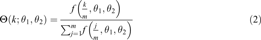
where

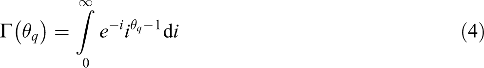
is the gamma function in standard form. The equal weighting scheme can be obtained when
The MIDAS model can also be extended to the multiple-lag form of predictor F as

where
In the MIDAS model, in addition to introducing the lags of the predicted variable y, we focus on the information of the high-frequency factor
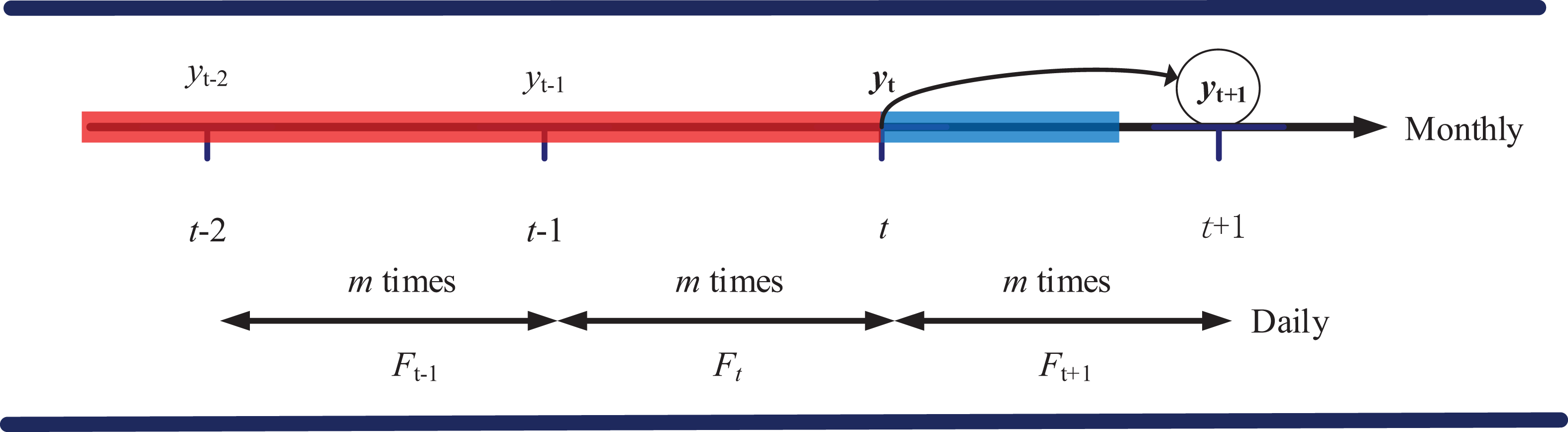
Forecast timeline.
Dynamic factor model
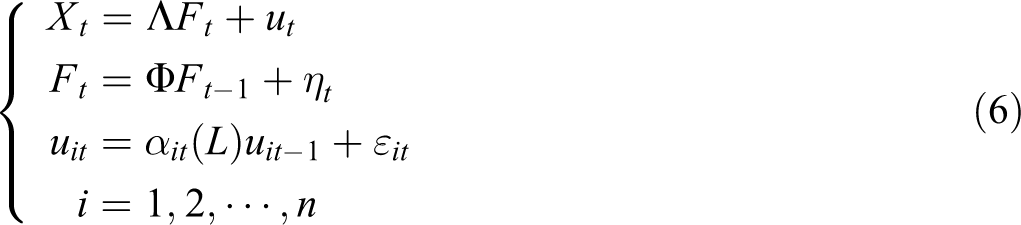
In this work, the dynamic factor model is introduced to obtain comprehensive variables from large panels of search data. The basic purpose of the dynamic factor model is to obtain a few common factors through dimension reduction. These few factors can explain the main part of the original variable information and avoid information redundancy, overfitting, and multicollinearity (Li et al., 2017). Research shows that the introduction of the dynamic factor model is beneficial to the prediction of macroeconomic variables (Forni et al., 2003; Li et al., 2017).
Supposedly, a large data set X with p variables will be used for prediction. Each variable has n observations and assumes that
The number of factors is determined by the suggestion of Bai and Ng (2002), and the parameters are determined by the maximum likelihood method. Once the dynamic factors are obtained, they are taken into the MIDAS model to carry out a single-factor model prediction experiment. The final forecasts are obtained through the forecast combinations.
Forecast combinations
To make full use of the information of each common factor, the forecast combinations are introduced to combine the prediction results of individual MIDAS with a single factor without increasing the estimated parameters of the model and maintaining its parsimony. Previous studies have agreed that forecast combinations with preset weighting scheme can improve the prediction accuracy of a single model (Timmermann, 2006) and can deal with the instability and structural mutation of the univariate model (Watson and Stock, 2004)
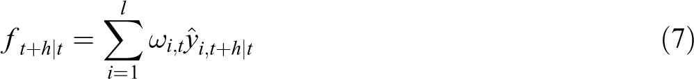
where
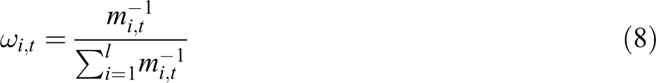
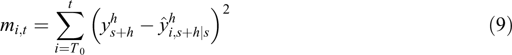
where T0 is the time point of the first out-of-sample observed value, and
Forecast evaluation
To evaluate the forecast power of the constructed hybrid forecast approach, the AR model and autoregressive distributed lag (ADL) model are introduced as the benchmark models, which can be expressed as follows:
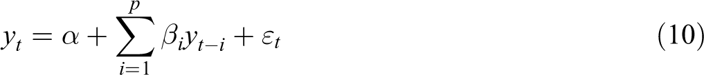

AR uses historical observations of hotel occupancy for prediction, and the lag order p is determined by using AIC and BIC criteria. ADL introduces public factor exogenous vector X and their lag terms based on AR. To ensure frequency consistency, the high-frequency factor obtained is converted into a low-frequency factor variable by using the equal weighting scheme, and the lag number is determined according to the AIC and BIC criteria. The parameters of AR and ADL are estimated by the least square method. In addition, the individual MIDAS model with a single factor is also used as a benchmark model to examine the effectiveness of the combination forecasts. Root mean square error (RMSE), mean absolute percentage error (MAPE), and coefficient of determination (R) are used as the standards to measure prediction performance. The expressions of the three indicators are as follows:


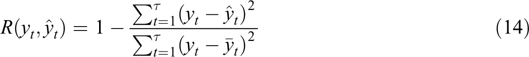
where yt and
RMSE is an absolute index, and its value ranges from zero to infinity. When the predicted value and the real value are completely consistent, it is equal to 0; greater error entails greater value. MAPE is a relative index with a range of
To evaluate the predictive power of non-nested models, the Diebold and Mariano (DM) method was used to verify whether there exists a significant difference between two non-nested forecast models (Diebold and Mariano, 1995). To achieve this goal, the following statistical hypotheses were put forward:
A loss function

When comparing predictive capabilities, the DM test introduces the loss differential:

Equation (16) is used to construct the DM test statistics (Diebold and Mariano 1995):
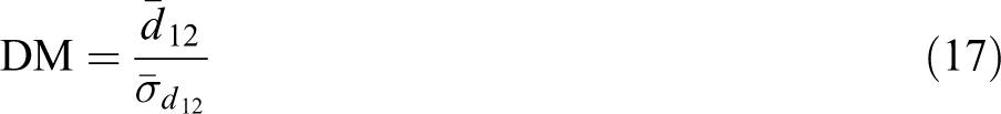
where
Hybrid MIDAS forecasting approach
As shown in Figure 2, the hybrid MIDAS forecasting approach integrating a dynamic factor model and forecast combinations is constructed through five steps for empirical analysis. The specific steps are as follows:
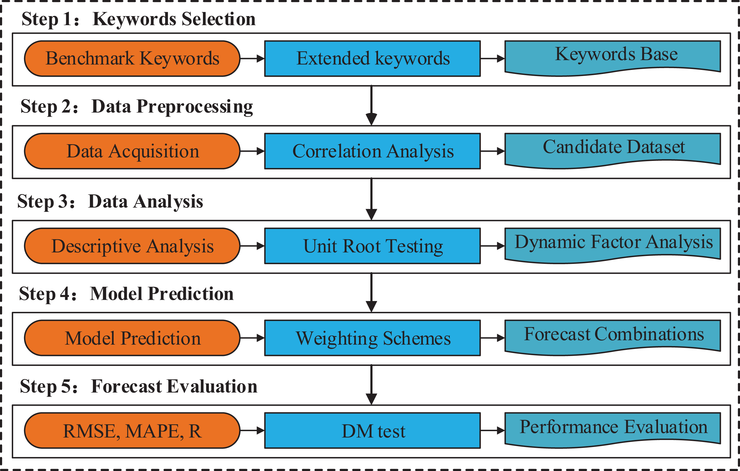
Flow diagram of the hybrid mixed-data sampling approach.
Step 1: Key word selection. On the basis of Yang et al. (2015) and Zhang et al. (2020), we use the search engine automatic recommendation technology provided by Baidu to obtain the benchmark key words. These benchmark key words include all aspects of information queries related to the six elements of a tourist destination. Then, the other key words related to the benchmark terms are searched circularly to form a database of key words.
Step 2: Data acquisition and preprocessing. First, the observations of all key words in the key word database are obtained. To obtain the key word variables with prediction ability before dynamic factor analysis, irrelevant queries must be eliminated. To achieve this goal, Pearson cross-correlation analysis is carried out to identify the search data related to the predicted variables (Zhang et al., 2017) and form the initial experimental data set. In this study, the key word variables are converted using an equal weighting scheme to conduct the Pearson cross-correlation analysis.
Step 3: Data analysis. To explore the basic characteristics of each variable, descriptive statistical analysis is conducted. Considering the requirements of the model for the stationarity of time series, the Augmented Dickey–Fuller (ADF) unit root test is carried out for all variables. Meanwhile, unstable variables are transformed by the difference method. The dynamic factor model is used to obtain factor variables from all the search series. Given the requirement of the equal sampling rate of high-frequency variables in each month, the observation value of each factor in each month is adjusted to 30 days. When a month has 31 days, the observation of the 30th day is replaced by the average value of the last 2 days. The interpolation method is used to supplement the data every February. The adjusted public factors and predicted variables are used as experimental data sets.
Step 4: Prediction experiment. The experimental data set is divided into two parts viz. the training section and the test section, which are used for the model estimation and prediction tests, respectively. A single common factor is taken into the MIDAS for prediction experiments, and the prediction results of each single-factor MIDAS model are combined to generate the final forecasts.
Step 5: Forecast evaluation. The prediction accuracy between the proposed prediction method and the benchmark models is evaluated by using predictive performance metrics and DM significance tests.
Empirical results
Data acquisition and preprocessing
To evaluate the prediction performance of the constructed hybrid prediction method, this study takes Sanya, a famous tourist destination in China’s Hainan province, as a case study. The city received 23.9633 million overnight tourists in 2019, which was an increase of 10.0% over the previous year. The average occupancy of the tourist hotels was 71.81%—an increase of 0.36% over the previous year. The monthly data of hotel occupancy is collected from the official website of Sanya (http://lwj.sanya.gov.cn/), covering January 2011 to December 2019. For convenience, the values of hotel occupancy are expressed in decimals with values range from 0 to 1.
As the econometric model should be driven by demand theory, price and income should be used as the forecast variables in the model. However, the official database does not directly provide historical data on average room rates. The consumer price index (CPI) can reflect changes in price levels, but the selected empirical case only provides CPI data after January 2013 (the time range of experimental data was from January 2011 to December 2019), and there is a serious lack of data every month. In addition, the disposable income data collected only include the annual data for nine years, and no suitable method has been found to forecast monthly tourism demand by using the annual data as the prediction variable. Therefore, following the forecasting approach of Bangwayo-Skeete and Skeete (2015) and Volchek et al. (2019), this study only uses the search data for prediction research.
The Internet search data are collected from Baidu (http://index.baidu.com), which provides daily and weekly search data. These search queries are based on the search volume of netizens on Baidu. According to step 1 of the prediction approach, we search for key words related to Hainan and Sanya tourism given that Sanya is the core tourist city of Hainan. These key words include food and accommodation, transportation, scenic spots, shopping, and entertainment. Finally, 58 key words are collected to form a key word database.
According to step 2, the daily search volume time series of 58 key words over the period under consideration is collected. To exclude the information that is not related to the predicted variables before performing dynamic factor analysis, Pearson cross-correlation analysis is employed to calculate the maximum correlation coefficient between the hotel occupancy and the 0–12 order lag variables of each key word variable. The selection of the maximum lag order is 12 considering the periodicity of the monthly data. To reduce the information loss, the threshold of the correlation coefficient is set to 0.6, and 14 key words are reserved. There are three reasons to set the threshold to 0.6. First, the correlation coefficient between key word variables and forecasted variable is statistically significant at least at 10% level (the original assumption is that the correlation coefficient is equal to 0) when the correlation coefficient is greater than 0.6. However, the correlation coefficient between key word variables and forecasted variable is not statistically significant when the correlation coefficient is less than 0.6, even many key word variables are negatively correlated with the forecasted variable. Second, the key word variables with correlation coefficient below 0.6 do not show the same seasonal characteristics and periodic fluctuations as the forecasted variables, and these key words contain much noise, which can not provide useful information for forecasting. Finally, if the threshold is set to 0.7, the three key word variables of “Hainan specialty,” “Hainan self-driving travel,” and “Sanya accommodation” that have significant correlation with the predicted variable may be excluded from the experimental data set. Through preliminary experiments, we found that excluding any one of these three key words will reduce the correlation between the common factors and the predicted variable, which further leads to information loss of key word variables and affects the prediction accuracy. Therefore, to keep the important characteristics of these three key words as much as possible, the threshold is not greater than 0.6.
The outcomes of the cross-correlation analysis are displayed in Table 1. The table shows a strong correlation between information search terms and hotel occupancy, and the optimal lag order of most variables is 1 to 3. The maximum lag order is 7, indicating that most information search behavior occurs approximately two months before trip. These key words are the leading indicators of hotel occupancy.
Pearson correlation analysis between key word variables and predicted variable.
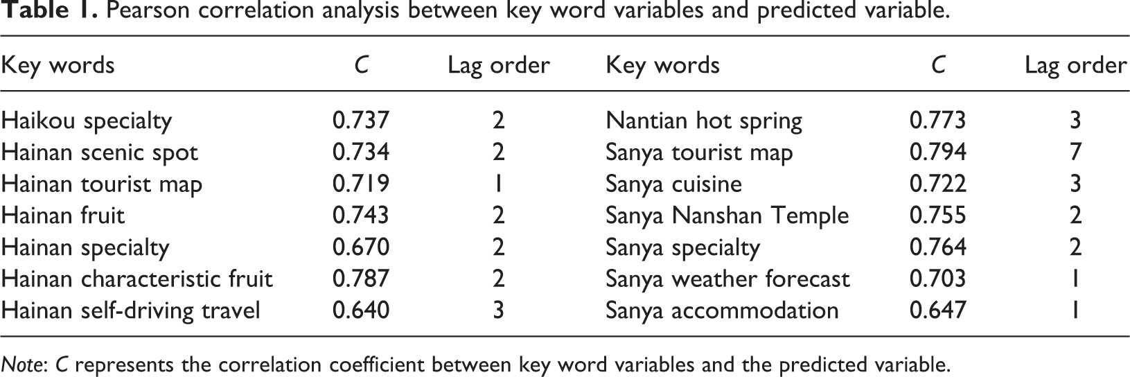
Note: C represents the correlation coefficient between key word variables and the predicted variable.
Figure 3 further intuitively presents the trend between the hotel occupancy and the two key word variables of “Hainan fruit” and “Sanya accommodation” among the 14 key variables. It presents consistent fluctuation characteristics and a close correlation between the daily key word variables and the monthly hotel occupancy. Given the seasonality, the tourist flow is at its peak from January to August every year, and the information search also exhibits similar traits. However, the fluctuation characteristics of different key words in a local area show heterogeneity, which means that different key words reflect potential tourists’ demand from various aspects and provide different characteristic information for hotel occupancy prediction. This observation prompts us to explore the validity of these high-frequency search data in the hotel occupancy forecast further.
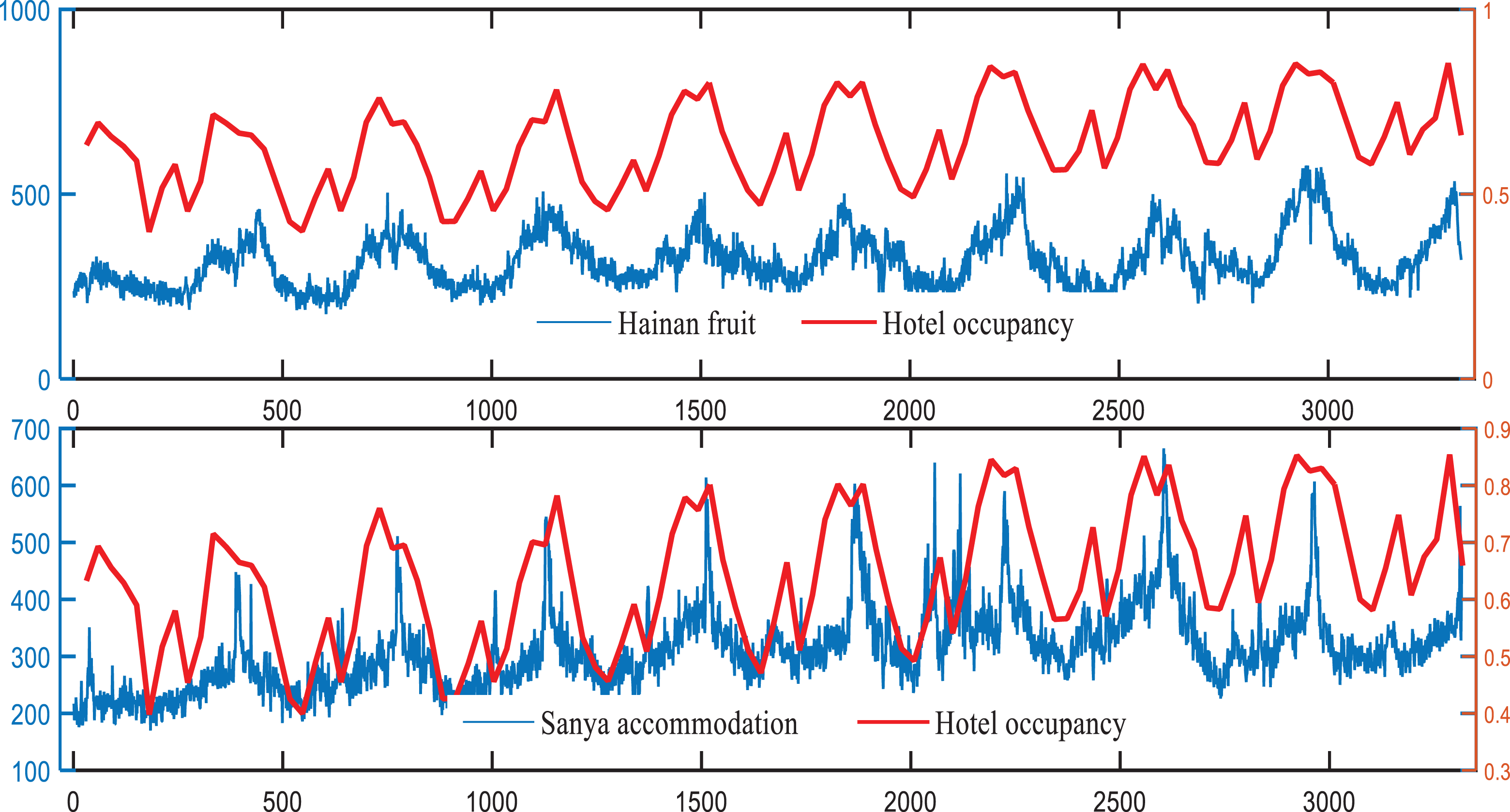
Fluctuation trend between “Hainan fruit” as well as “Sanya accommodation” and hotel occupancy.
Data analysis
According to step 3, the descriptive statistical analysis and stable analysis are carried out for 14 key words and predicted variables. In this work, the stability of variables is tested by using the ADF test. The results of the descriptive statistical analysis and the ADF test are presented in Table 2. Test results (the last two columns of Table 2) show that except for “Sanya specialty” rejecting the original hypothesis at the 5% level, all other time series reject the original hypothesis at the 1% level, thus indicating that all variables meet the stationarity.
Descriptive statistical analysis and ADF test of all variables.
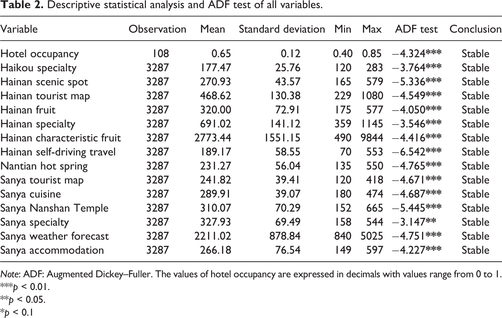
Note: ADF: Augmented Dickey–Fuller. The values of hotel occupancy are expressed in decimals with values range from 0 to 1.
***p < 0.01.
**p < 0.05.
*p < 0.1
For dimensionality reduction, the dynamic factor model is used to extract threshold from 14 key word variables. Finally, two common factors denoted by F1 and F2 are obtained, which explain more than 80% of the original variable information. Moreover, according to the load matrix of dynamic factor analysis results, the correlation coefficients between F1 and the key word variables of “Hainan tourist map,” “Hainan fruit,” “Hainan characteristic fruit,” “Hainan self driving travel,” “Sanya tourist map,” “Sanya weather forecast,” and “Sanya accommodation” all exceed 0.67. This means that F1 mainly explains the information about eating, accommodation, and transportation related to the destination. The correlation coefficients between F2 and the key word variables of “Haikou specialty,” “Hainan specialty,” “Nantian hot spring,” “Sanya cuisine,” “Sanya Nanshan Temple,” and “Sanya specialty” all exceed 0.71, which suggests that F2 mainly captures the information about travelling, shopping, and entertainment related to the destination.
Given that the sampling rate of common factor variables in each month is inconsistent, the common factor variable is adjusted according to step 3. In addition, the sampling rate of each month after adjustment is 30 days. The adjusted common factors and the predicted variables constitute the experimental data set. To carry out the prediction experiment, the experimental data set is divided into two sections: the initial data sample from January 2011 to December 2018 as the training section for model estimation and the data from January 2019 to December 2019 as the testing section for forecasting.
Results and discussions
For convenience, MIDAS-1 refers to the MIDAS model with the common factor F1 as a high-frequency prediction variable, and MIDAS-2 refers to the MIDAS model with the common factor F2 as a high-frequency prediction variable. The constructed hybrid forecasting approach is represented as MIDAS-C, which is the weighted average of MIDAS-1 and MIDAS-2. In the process of prediction experiments, a rolling window scheme is applied for all the models. AIC and BIC criteria are used to determine the lag order of the hotel occupancy and the high-frequency factor variables. In the weighting scheme, only two parameters in the Beta function are estimated, and the parameters of all MIDAS models are estimated by the nonlinear least square method.
Figure 4 shows the prediction curves of each model on the test set by one step and multiple steps (h = 1, 3, 6, 10) ahead horizons. The figure shows that the fitting power of each forecasting technique on the test section is preferable. Among them, the deviation of the MIDAS-C prediction curve from the expected value is smaller, which shows that the prediction method constructed in this study has a good fitting ability. The fitting effect of AR amongst the benchmark model is the worst. To illustrate the predictive ability of each model on the test set further, the predictive performance index values of each model must be compared.
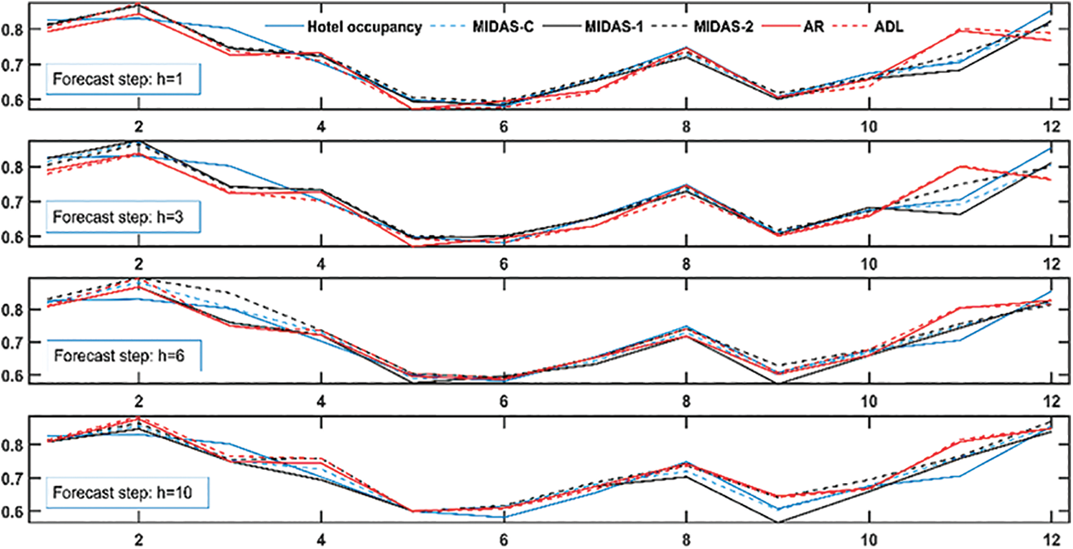
Comparison of one step and multiple steps ahead forecasts of forecast models.
Tables 3 and 4 show the comparison of the one step and multiple steps ahead statistical index (RMSE and MAPE) values of each model on the test set. As shown in Tables 3 and 4, MIDAS-C performs best on the two indicators, which means that the prediction power of the proposed approach is better than that of its competitors. Specifically, compared with the AR and ADL models, the improvement rate (IR) of MIDAS-C on RMSE and MAPE by all forecast horizons exceeds 33% and 25%, respectively. Compared with the univariate MIDAS model, the prediction accuracy of MIDAS-C on RMSE and MAPE by all forecast horizons increased by approximately 9% and 17%, respectively.
Comparison of RMSE values of each model for the Sanya data set.
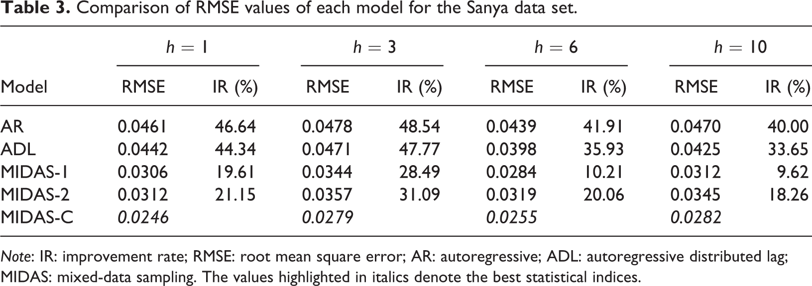
Note: IR: improvement rate; RMSE: root mean square error; AR: autoregressive; ADL: autoregressive distributed lag; MIDAS: mixed-data sampling. The values highlighted in italics denote the best statistical indices.
Comparison of MAPE values of each model for the Sanya data set.
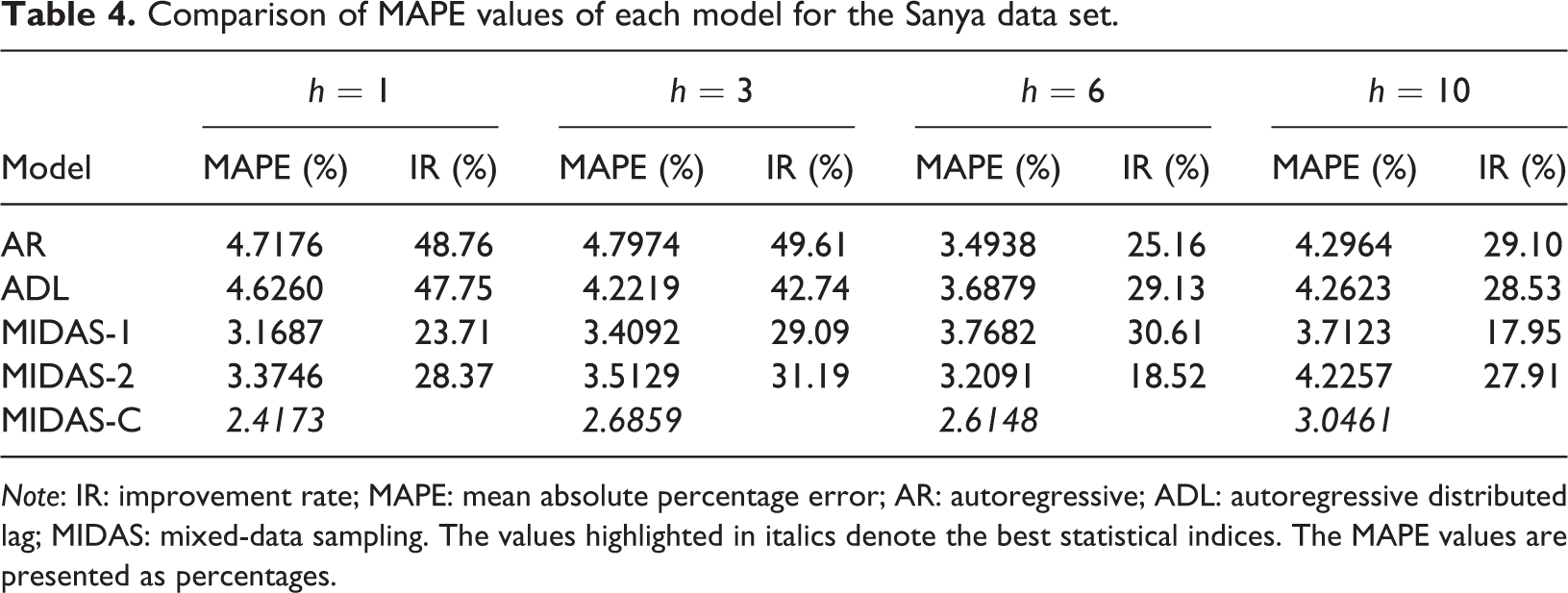
Note: IR: improvement rate; MAPE: mean absolute percentage error; AR: autoregressive; ADL: autoregressive distributed lag; MIDAS: mixed-data sampling. The values highlighted in italics denote the best statistical indices. The MAPE values are presented as percentages.
Table 5 shows the comparison of the one step and multiple steps ahead R values of each model on the test set. As shown in Table 5, the fitting ability of the prediction model constructed in this research has varying degrees of improvement on the other forecast horizons except the 10-step ahead forecasts compared with its competitors, it is approximately 0.9% higher than AR and ADL and at least 1% higher than the single-factor MIDAS model.
Comparison of R values of each model for the Sanya data set.
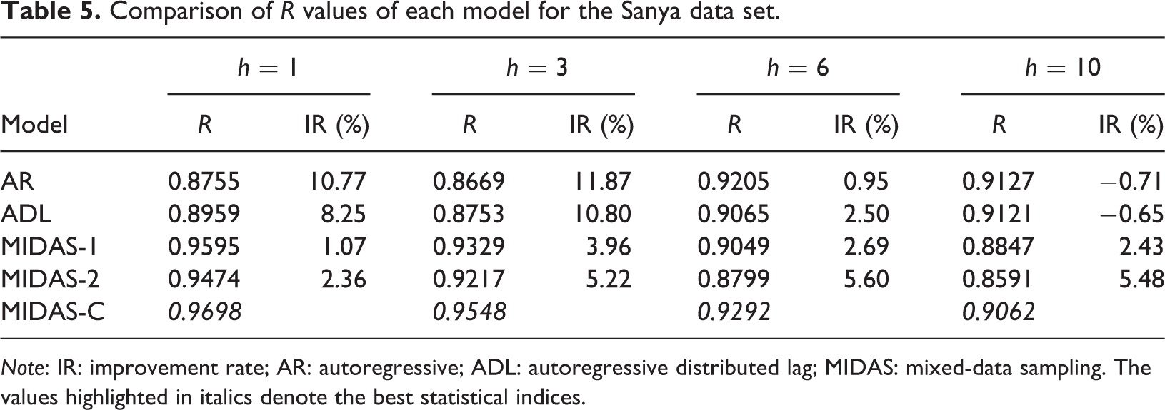
Note: IR: improvement rate; AR: autoregressive; ADL: autoregressive distributed lag; MIDAS: mixed-data sampling. The values highlighted in italics denote the best statistical indices.
To verify further whether the improvement of prediction accuracy is significant, we carried out a DM test on each forecast step, and the outcomes are shown in Table 6. The test statistics and p-value in Table 6 show that on one step and multiple steps ahead prediction results reject the null hypothesis at different significance levels (1% statistical significance level in most cases). This outcome indicates that the forecast accuracy of MIDAS-C is significantly different from that of other models.
Tests of equal predictive ability with the DM test for the Sanya data set.
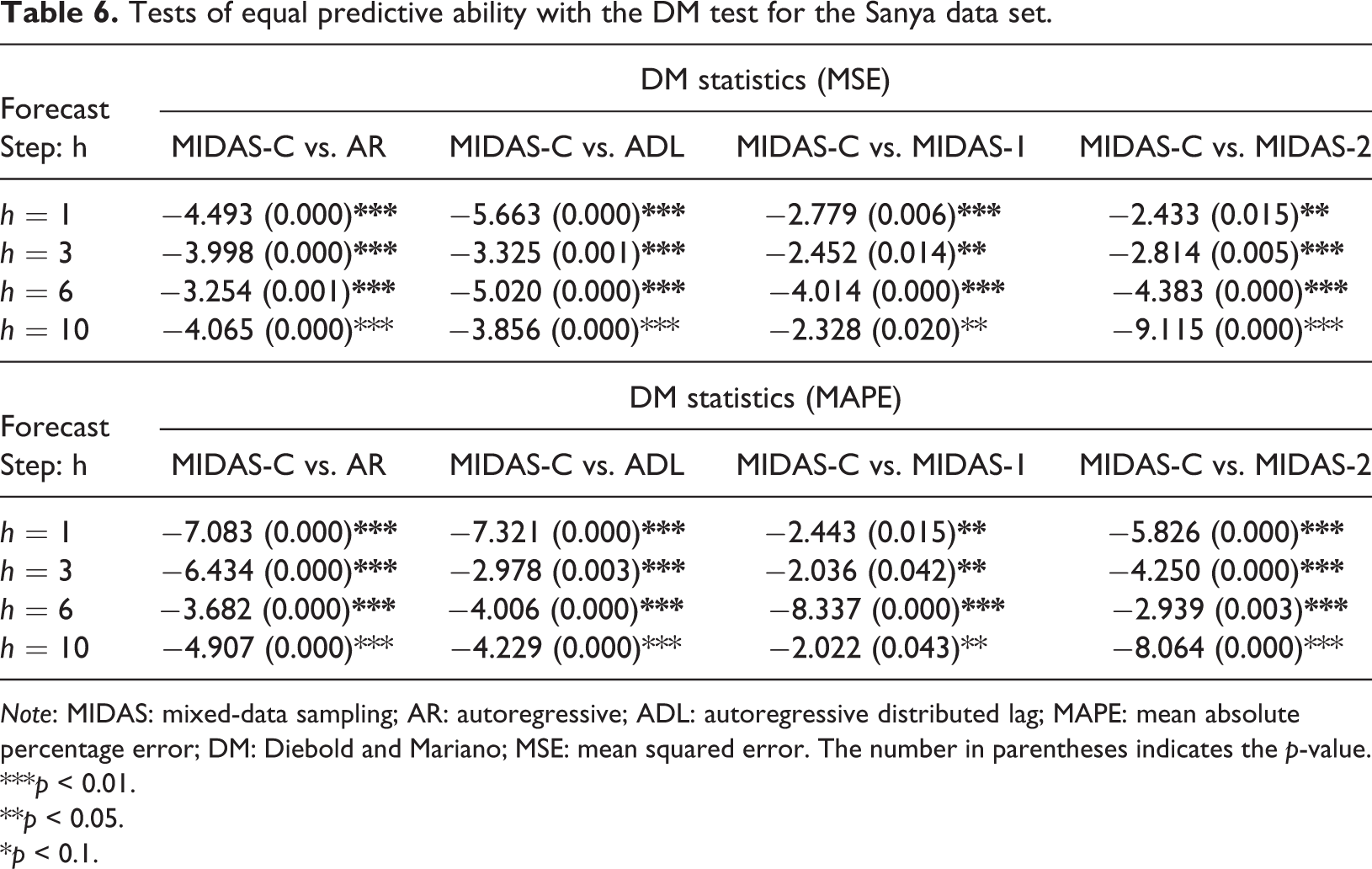
Note: MIDAS: mixed-data sampling; AR: autoregressive; ADL: autoregressive distributed lag; MAPE: mean absolute percentage error; DM: Diebold and Mariano; MSE: mean squared error. The number in parentheses indicates the p-value.
***p < 0.01.
**p < 0.05.
*p < 0.1.
In summary, the aforementioned analysis reveals that the prediction accuracy of the proposed hybrid MIDAS approach integrating a dynamic factor model and forecast combinations is significantly improved compared with its competitors. Moreover, the results confirm that daily search data is helpful to the hotel occupancy prediction, thus adding evidence to the conclusions of Bangwayo-Skeete and Skeete (2015) and Qin and Liu (2019). This confirmation is attributed to the following facts. First, the AR model uses only the historical information of the predicted variable and does not add the key word variables with predictive ability. Its prediction ability is significantly lower than that of the MIDAS-C. Second, the ADL model converts two high-frequency common factor variables into monthly variables by equal weighting scheme, thus losing the dynamic characteristic information of the original high-frequency data (Kim and Swanson, 2017) and resulting in its prediction ability to be significantly lower than that of the proposed MIDAS-C. Finally, MIDAS-C has stronger predictive ability than the two univariate MIDAS models, thus indicating that the forecast combinations can significantly improve the forecasting accuracy. This outcome is consistent with the conclusions of Timmermann (2006), as the forecast combinations are more stable than the univariate MIDAS model (Watson and Stock, 2004). Additionally, the constructed method integrates the main feature information of the original key word variables.
Another case study
To enhance the generalization of this study, we take Beijing as another numerical example. The monthly data of hotel occupancy is collected from the Wind database, a leading financial database curated in China, and the search engine data are collected from Baidu. We used the same detailed forecasting procedure described in the “Hybrid MIDAS forecasting approach” subsection for the forecasting experiment over the same time span. Through the first three steps of the prediction framework, 10 key word variables with prediction ability are obtained, and two common factors are extracted by using the dynamic factor model. The forecasting results are shown in Tables 7, 8, and 9. The results show that MIDAS-C performs better than the other indicators and forecasting steps except the ADL model in the R index of the 6-step ahead horizon.
Comparison of RMSE values of each model for the Beijing data set.
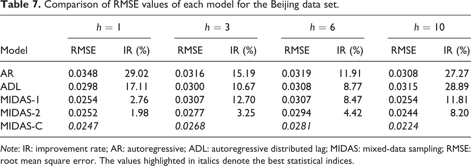
Note: IR: improvement rate; AR: autoregressive; ADL: autoregressive distributed lag; MIDAS: mixed-data sampling; RMSE: root mean square error. The values highlighted in italics denote the best statistical indices.
Comparison of MAPE values of each model for the Beijing data set.
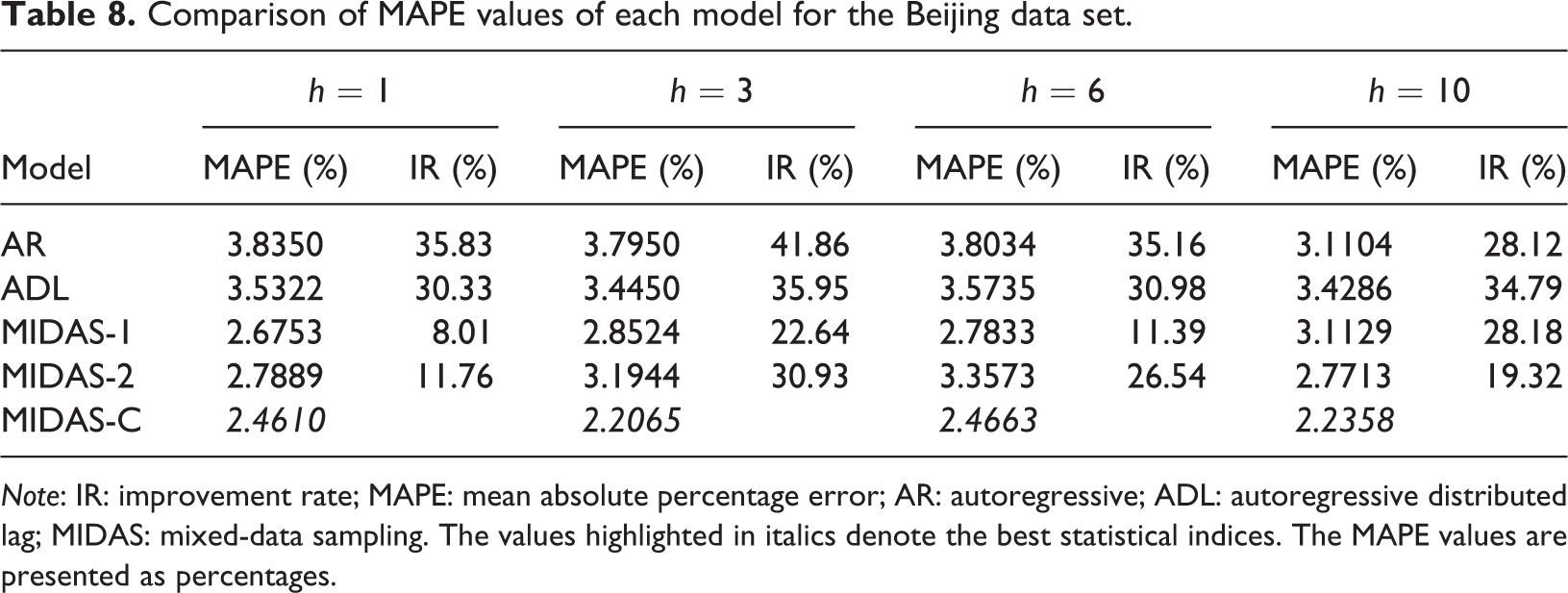
Note: IR: improvement rate; MAPE: mean absolute percentage error; AR: autoregressive; ADL: autoregressive distributed lag; MIDAS: mixed-data sampling. The values highlighted in italics denote the best statistical indices. The MAPE values are presented as percentages.
Comparison of R values of each model for the Beijing data set.
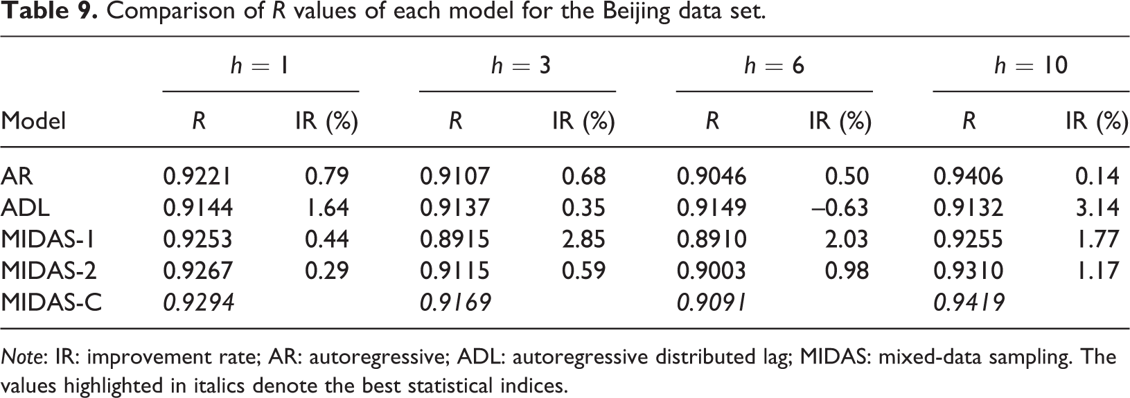
Note: IR: improvement rate; AR: autoregressive; ADL: autoregressive distributed lag; MIDAS: mixed-data sampling. The values highlighted in italics denote the best statistical indices.
The significance test results in Table 10 show that, in terms of the MSE index, the forecasting accuracy of MIDAS-C is significantly different from that of other models except MIDAS-2 on three-step ahead forecasts. In terms of the MAPE indicator, the results suggest that the forecasting accuracy of MIDAS-C is significantly different from that of other models on all forecast horizons. Overall, the empirical analysis once again suggests that the developed approach can produce preferable and robust forecasting results.
Tests of equal predictive ability with the DM test for the Beijing data set.

Note: MIDAS: mixed-data sampling; AR: autoregressive; ADL: autoregressive distributed lag; MAPE: mean absolute percentage error; DM: Diebold and Mariano; MSE: mean squared error. The number in parentheses indicates the p-value.
***p < 0.01.
**p < 0.05.
*p < 0.1.
Conclusions and implications
Accurate demand forecasting is of utmost help in scientific decision-making to hospitality and tourism-related industries. With the popularity of the Internet, web information search objectively reflects consumers’ potential demand and provides a reliable source of data for demand forecasting. However, forecasting accuracy is affected by the inconsistency of data frequency and increasing key word variables. In this study, we use the dynamic factor model to obtain two factors and directly model the monthly hotel occupancy and daily key word variables in the hybrid MIDAS framework. Then, we construct two single-factor MIDAS models for the two common factors. Then, the final forecasts are obtained by forecast combinations. The results show that compared with the baseline models, the proposed hybrid approach can significantly improve accuracy while maintaining parsimony and flexibility, and the forecast results are more robust. Moreover, MIDAS-C alleviates the fitting problem to a certain extent. We conclude that incorporating daily search data into the constructed predictive model can lead to improvements in the monthly forecasts of hotel occupancy over its baseline models.
The contribution of this work to the existing research is mainly reflected in three aspects. First, the current hotel demand prediction method deals with the problem of equal frequency data prediction. Hence, the hybrid MIDAS approach integrating a dynamic factor model and forecast combinations in this study is reported to model the mixed-frequency data directly in a parsimonious and flexible way to reduce the prediction error rate of the model. Second, the effectiveness of the daily search data in the prediction of hotel occupancy is verified under the hybrid MIDAS approach for the first time. Lastly, to use the feature information of key word variables effectively, the dynamic factor model is used to obtain factor variables from large panels of daily search data. Moreover, the forecast combinations are used to obtain the final forecast values of the individual MIDAS model to improve the prediction ability further.
The research in this article has important theoretical implications. First, given the inconsistent frequency of the predicted variables and the prediction variables, the hybrid MIDAS approach is introduced to model the mixed-frequency data directly, which ensures the parsimony and flexibility of the modeling. Second, the dynamic factor model is introduced to extract the feature information from large amounts of search engine data. The original variable feature information is retained, while the dimension reduction is achieved. Thus, the model estimation is parsimonious. Finally, the forecast combinations are constructed to avoid the instability of the single-factor MIDAS model and improve the prediction ability.
This research has practical implications for policy makers, researchers, and practitioners. In particular, the results show that the daily key word variables contain useful feature information. The data is updated daily, while the frequency of hotel occupancy is updated monthly. Generally, the hotel occupancy observations of the current month are released in the middle and late periods of the following month. Therefore, before the official data are released, the current month’s daily search data is available and can be used to predict the current month’s hotel occupancy rate (nowcasting) in advance. From the policy point of view, forecast results can provide the necessary information support to policy makers and business managers in various aspects, such as planning, marketing, income management, investment, and annual budget. For example, in the off-season and peak season, hotels use forecast results to implement additional scientific promotion plans, ensure a reasonable allocation of hotel resources, and avoid unnecessary wastage. With regard to the prediction method, the prediction approach constructed in this work can be generalized to other demand forecasts, such as tourist flow and revenue, to solve the frequency inconsistency and the large amounts of key word variables to reduce the prediction error rate.
However, given the data collection restrictions, the experimental data set does not include search data from other search engines and other hospitality and tourism-related series such as macroeconomic data and various online review records. Integrating other data sources to verify and compare the performance of demand forecasting would be a direction of further research.
Footnotes
Acknowledgment
The authors are grateful to the editors and the anonymous reviewers for their valuable comments and suggestions.
Declaration of conflicting interests
The author(s) declared no potential conflicts of interest with respect to the research, authorship, and/or publication of this article.
Funding
The author(s) disclosed receipt of the following financial support for the research, authorship, and/or publication of this article: This research was funded by the Humanities and Social Science Fund of Ministry of Education of China, grant number 20YJC630202 and supported by a grant from State Key Laboratory of Resources and Environmental Information System.