UK overseas visitors: Seasonality and persistence

Abstract

This article analyses seasonality and persistence in the number of UK overseas visitors applying a fractional integration framework to (monthly and quarterly) data from 1986 to 2017. The results indicate that long memory is present in the series and the degree of persistence is higher for seasonally adjusted data, with shocks having transitory but long-lasting effects.

Introduction

This article analyses seasonality and persistence in the number of UK overseas visitors applying a fractional integration framework to (monthly and quarterly) data from 1986 to 2017. These two features are very common in tourism-related series, and despite the existence of numerous studies analysing them, there is still no consensus on the most appropriate empirical framework to apply. Seasonality can be modelled either deterministically (using seasonal dummy variables) or stochastically; in the latter case, either stationary Auto Regressive Moving Average (ARMA) seasonal models or seasonal unit roots (as in Dickey et al., 1984 or Hylleberg et al., 1990) can be used. Examples of tourism studies using these techniques are Kim and Moosa (2001), Alleyne (2006), Shen et al. (2009), Lean and Smyth (2008) and so on. As for persistence, unit root methods (e.g. Dickey and Fuller, 1979; Phillips and Perron, 1988; Elliot et al., 1996; etc.) have been widely used to assess whether the effects of shocks are transitory or permanent and the dynamic adjustment process (Narayan, 2003; Perles-Ribes et al., 2016).

The fractional integration model estimated in the present note is more general than others only allowing for integer degrees of integration, namely either 0 (in the case of stationary series) or 1 (in the case of nonstationary unit root processes). Fractional integration methods have already been applied to analyse tourism data in a few other studies such as Cunado et al. (2004), Nowman and Van Dellen (2012) and Gil-Alana et al. (2015). Using this approach, we show that the degree of persistence of the series changes when applying standard seasonal adjustment procedures. This is the key finding of our note, namely the degree of persistence of the series, measured by the differencing parameter, changes when seasonal adjustment is carried out. The remainder of the article is structured as follows: “Methodology” section outlines the methodology; “Data and empirical results” section describes the data and presents the main empirical results, while “Conclusions” section offers some concluding remarks.

Methodology

Let {y_t, t = 1, 2,…, T} denote the time series of interest. Then consider the following model

$y_t={\beta }_0+{\beta }_{1}t+x_t,{(1-L)}^d{x}_t=u_t,t=1,2,\dots$

1

where β₀ and β₁ are unknown and stand respectively for the intercept and the coefficient on a linear time trend, and x_t is assumed to be I(d), where d can be any real value, thus also allowing for fractional degrees of integration. In this context, u_t is by definition I(0) and is assumed to follow a seasonal AR process of the following form

$\varphi (L^s)u_t={\epsilon }_t,t=1,2,\dots$

2

where L^s is the seasonal lag operator (L^su_t = u_t−s) and ε_t is a white noise process. The chosen specification includes stochastic seasonality because we find no evidence of deterministic seasonality when estimating simple models with seasonal (quarterly and monthly) dummy variables, all their coefficients not being statistically significant (these results are not reported for brevity’s sake).

When the data are seasonally adjusted (SA), instead of (2) we assume that u_t is autocorrelated as in the exponential spectral model of Bloomfield (1973), which is a non-parametric approach of approximating ARMA models with a small number of parameters. The estimation is carried out using the Whittle function in the frequency domain (Dahlhaus, 1989; Robinson, 1994) and the Fortran programme codes of are available from the authors upon request.

Data and empirical results

The series analysed are the number of UK overseas visitors (All visits, thousands), quarterly and monthly, non-seasonally adjusted (NSA) and SA, for the time period 1986 (m1/q1) − 2017 (m12/q4). The data were obtained from the Office for National Statistics (Overseas travel and tourism time series (OTT)).

Figure 1 displays the series of interest. These appear to be highly persistent, and seasonal patterns are very noticeable in the case of the seasonally unadjusted data. Tables 1 and 2 report the results for the monthly and quarterly data, respectively. In all cases, we estimate the model given by equation (1); as already mentioned, the error term is assumed to follow a seasonal autoregressive process in the case of the raw data, and Bloomfield’s (1973) autocorrelation model in the case of the SA ones. Both tables show the estimated values of d along with the 95% confidence intervals for the three standard cases of (i) no deterministic terms (i.e. β₀ = β₁ = 0 a priori in (1)), (ii) with an intercept only (β₀ unknown and β₁ = 0), and with an intercept and a linear trend (both β₀ and β₁ estimated from the data), with the significant coefficients (on the basis of the t-statistics) in bold. A time trend appears to be required in all cases.

Figure 1.

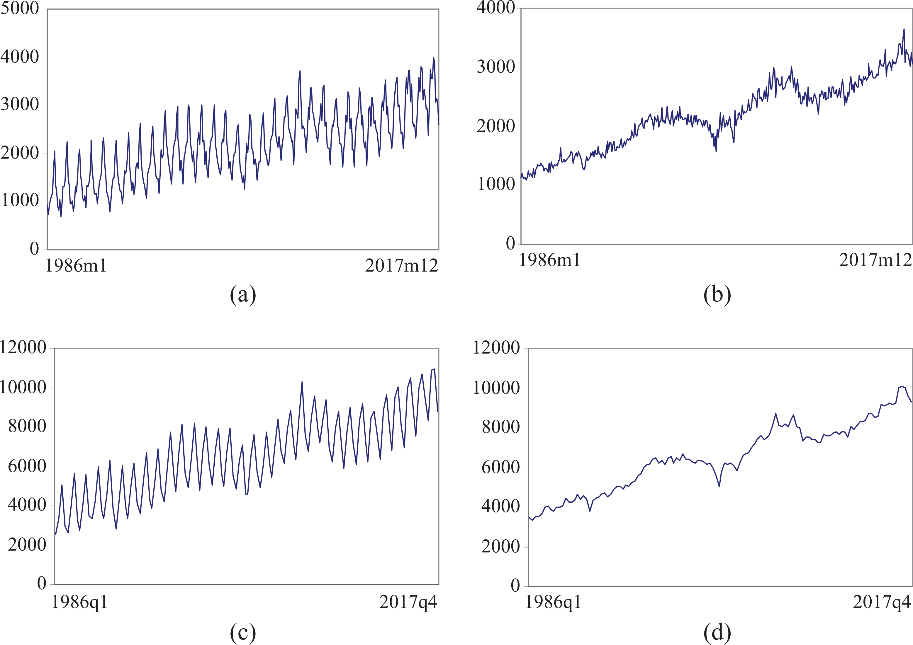
Time series plots. (a) Non-seasonal monthly data, (b) seasonally adjusted monthly data, (c) non-seasonal quarterly data and (d) seasonally adjusted quarterly data.

Table 1.

Estimated coefficients for the monthly data.

Monthly data	No terms	An intercept	A linear time trend
NSA	0.36 (0.29, 0.48)	0.49 (0.46, 0.54)	0.36 (0.29, 0.43)
	ρs=12 = 0.906	ρs=12 = 0.892	ρs=12 = 0.906
SA (no autocorrelation)	0.63 (0.57, 0.69)	0.57 (0.54, 0.61)	0.50 (0.46, 0.56)
SA (autocorrelated)	0.82 (0.73, 0.94)	0.73 (0.65, 0.84)	0.70 (0.62, 0.83)

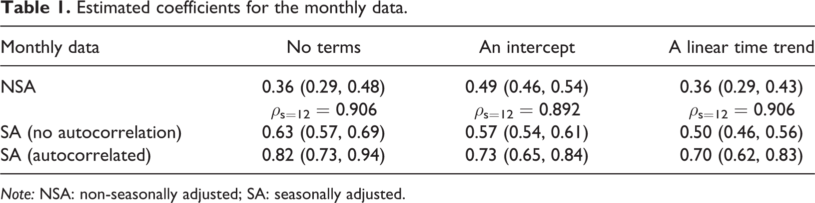
Note: NSA: non-seasonally adjusted; SA: seasonally adjusted.

Table 2.

Estimated coefficients for the quarterly data.

Quarterly	No terms	An intercept	A linear time trend
NSA	0.35 (0.28, 0.46)	0.60 (0.53, 0.70)	0.44 (0.30, 0.60)
	ρs=12 = 0.950	ρs=12 = 0.965	ρs=12 = 0.962
SA (no autocorrelation)	0.87 (0.77, 1.00)	0.86 (0.76, 1.02)	0.85 (0.73, 1.01)
SA (autocorrelated)	0.87 (0.68, 1.06)	0.74 (0.61, 0.98)	0.73 (0.50, 1.00)

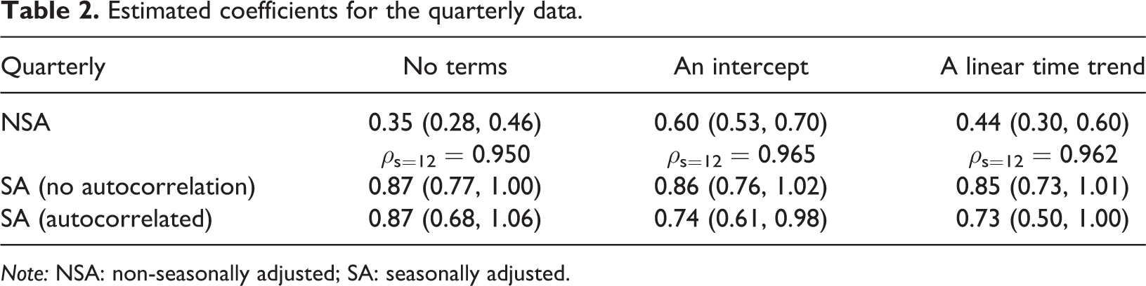
Note: NSA: non-seasonally adjusted; SA: seasonally adjusted.

Table 1 shows that for the raw monthly data, the estimated value of d is equal to 0.36, and the confidence interval is above 0 and below 0.5, which implies stationarity and long-memory behaviour; further, the seasonal AR coefficient is extremely high (0.906). When the data are SA, the estimated value of d increases sharply, being equal to 0.50 with uncorrelated errors, and 0.70 under Bloomfield autocorrelation. In both cases, the confidence intervals only include values below 1, which implies mean-reverting behaviour.

Table 2 reports the estimates for the quarterly data; these are slightly higher than in the monthly case, but the general pattern is the same: for the raw data, the estimated value of d is 0.44 and the confidence interval excludes the cases of d = 0 and d = 1; for the SA data, the estimates of d are higher, namely 0.85 with white noise errors and 0.73 with autocorrelated errors (and closer to the unit root case).

Conclusions

In this short note, we have examined persistence and seasonality in the number of UK overseas visitors using fractional integration techniques. The main findings can be summarized as follows: the estimates of d are in the interval (0, 1) in all cases, thus suggesting the presence of long memory and fractionally integrated behaviour; higher values are obtained with the SA data and also for the quarterly rather than the monthly ones. This is an important result, which implies that a higher degree of persistence is found when using SA data, that is, the effect of shocks are estimated to last for longer in this case. From the point of view of policymakers whose task is to design appropriate policy responses to exogenous shocks, it would therefore be advisable to use unadjusted data to determine the degree of persistence and decide on how it should be handled using policy tools. In the case of UK overseas visitors, our results imply that shocks will have transitory but long-lasting effects, and such evidence should inform tourism policies.