Disproportionality often cannot range from zero to one: a note on the Gallagher index and a new normalised measure

Abstract

The Gallagher index is the most popular measure of disproportionality in political science. While many assume that it can range from 0 (perfect proportionality) to 1 (perfect disproportionality), I prove that its maximum value is constrained by the size of the party system. For any election with N_V effective vote-winning parties, the Gallagher index cannot exceed $\sqrt{(N_{V} + 1) / 2 N_{V}}$ . Given that party-system fragmentation has risen across developed democracies, researchers may sometimes wish to distinguish how disproportional an election was from how disproportional it could have been, given the size of the party system. As such, I propose a complementary index that runs from 0 to 1, no matter the degree of fragmentation.

Keywords

disproportionality electoral systems proportional representation Gallagher index party system fragmentation

Introduction

The Gallagher index (1991) is the most popular measure of disproportionality in political science. Recent work has used it to test how disproportional election results affect phenomena as varied as intra-party cohesion (Matakos et al., 2024), subjective health and well-being (Toshkov and Mazepus 2023), and corporate investment decisions (Amore and Corina 2021). The index has also had a life beyond the academy. For example, when Liberal Party leader Justin Trudeau committed to making 2015 Canada’s “last federal election conducted under the first-past-the-post voting system” (Liberal Party of Canada 2016, 8), it informed the work of the country’s Special Committee on Electoral Reform (2016). This dual role, as both an empirical measure and a practical tool, demonstrates the index’s more general importance.

In principle, the Gallagher index can vary between 0 (perfect proportionality) and 1 (perfect disproportionality). However, in this paper, I show that its actual maximum is often lower, since the size of the party system acts as a brake on the range of values that it can take. To this end, I prove that, at elections with N_V effective vote-winning parties, the Gallagher index has an upper bound of $\sqrt{(N_{V} + 1) / 2 N_{V}}$ . As the effective number of vote-winning parties tends to infinity, this bound then converges on $1 / \sqrt{2}$ . Given that party-system fragmentation has risen across developed democracies (Norris 2024), researchers may sometimes wish to distinguish how disproportional an election was from how disproportional it could have been, given the size of the party system. To account for this, I introduce a new normalised index that ranges from 0 to 1 no matter the degree of party-system fragmentation.

Measuring disproportionality

Disproportionality—the extent to which seat shares diverge from vote shares—has both normative and empirical consequences. Normatively, disproportionality challenges the equality of representation: the notion that each vote should carry equal weight (Dahl 1971). Indeed, McGann even goes so far as to argue that “proportionality is logically implied by the basic value of political equality, that is, by the concept of democracy itself” (2006, 35). Empirically, disproportionality occurs as a natural consequence of electoral system design, particularly the method of seat allocation (Duverger 1964). Where district magnitudes are large and electoral thresholds are low, elections tend to produce less disproportional outcomes than where they are not (Anckar 1997; Shugart and Taagepera 2017).

In general, there are two distinct perspectives on the measurement of disproportionality: one relative and one absolute. The relative perspective operationalises disproportionality in terms of the seats-to-vote ratio, the share of seats that some party wins divided by its share of the vote. The idea here is that, consistent with the equality of representation, disproportionality concerns the equal treatment of voters (Van Puyenbroeck 2008). If the same share of votes wins voters for party A more seats than voters for party B, then the latter are at a disadvantage. The difference perspective, instead, operationalises disproportionality in terms of the difference between vote and seat shares. Consequently, it treats disproportionality as a phenomenon that affects political parties instead. Despite compelling arguments in favour of relative measures of disproportionality like the Sainte-Laguë index (see Gallagher 1991; Goldenberg and Fisher 2019; Van Puyenbroeck 2008), absolute measures of disproportionality are now much more common in the study of electoral systems.

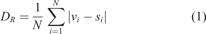
The oldest absolute measure of disproportionality comes from Rae (1971) and equals the average absolute difference between the vote share, v, and seat share, s, over all parties, N:

D_{R} = \frac{1}{N} \sum_{i = 1}^{N} | v_{i} - s_{i} |

(1)

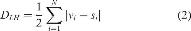
However, Rae’s measure applies an implicit downward bias on large party systems. To see why, consider that Rae’s index tends to zero in the limit where the number of parties tends to infinity, implying perfect proportionality no matter the distribution of votes and seats (Katz 1980). To overcome this problem, Loosemore and Hanby (1971) modified Rae’s index to ignore the number of parties (effectively treating disproportionality as an election-level phenomenon) and then multiplied the resulting index by 1/2 to rescale its output from 0 (perfect proportionality) to 1 (perfect disproportionality):

D_{L H} = \frac{1}{2} \sum_{i = 1}^{N} | v_{i} - s_{i} |

(2)

Though the Loosemore-Hanby index soon became the industry standard, it suffered from the opposite problem to Rae's index: it applies an upward bias for large party systems instead (Lijphart 1994). It also fails Dalton’s (1920) principle of transfers (the axiom that moving seats from over-represented to under-represented parties should always cause disproportionality to fall) and treats largest remainders systems as having more proportional outcomes by design (Gallagher 1991).

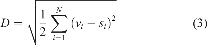
Gallagher’s (1991) ‘least squares’ index attempts to strike a balance between these two extremes. Rather than rely on the absolute difference between vote and seat shares—like Rae (1971) and Loosemore and Hanby (1971)—it relies on the squared difference instead, much like the method of least squares from which it takes its name. Gallagher’s index is also consistent with Dalton’s (1920) principle of transfers and balances under- and over-sensitivity to the number of parties by registering “a few large discrepancies more strongly than a lot of small ones” (Gallagher 1991, 40). We compute the index as follows:

D = \sqrt{\frac{1}{2} \sum_{i = 1}^{N} {(v_{i} - s_{i})}^{2}}

(3)

The Gallagher index is now the “industry standard for electoral analysis”(Goldenberg and Fisher 2019, 203), and several seminal works in electoral studies have used it to evidence their claims. For instance, Lijphart (2012, 1994) investigates how different electoral systems in use worldwide produce different levels of disproportionality. Likewise, Shugart and Taagepera (2017) provide an approximate predictive model of the index as part of their broader project on the institutional dynamics of electoral systems.

Though the Gallagher index may now be the “industry standard”, there is still much that we do not know about how it works. Consequently, a range of articles have attempted to address this gap in our knowledge (most notably Goldenberg and Fisher 2019; Van Puyenbroeck 2008; Taagepera and Grofman 2003). However, much like the rest of the literature, this work assumes that the Gallagher index can range from 0 (perfect proportionality) to 1 (perfect disproportionality). While this is true in principle, it is almost certainly not true in practice. This is because, as I show in the next section, the Gallagher index is sensitive to the overall size of the party system. And, as party systems fragment, they enforce strict constraints on the values that the index may take.

Establishing an upper bound on the Gallagher index

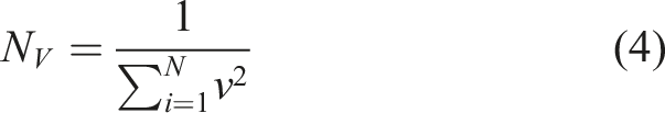
To show that the size of the party system constrains the Gallagher index, first recall that we can characterise any party system, no matter how large it may be, in terms of the effective number of parties (Laakso and Taagepera 1979). This quantity, most often used in studies of party-system fragmentation (e.g. Valentim and Dinas 2024), measures “the number of hypothetical equal-size parties that would have the same total effect on fractionalization of the system as have the actual parties of unequal size” (Laakso and Taagepera 1979, 4, emphasis in original). Where there are N actual vote-winning parties, we can compute the effective number of vote-winning parties, N_V, over some distribution of vote shares, v, such that:

N_{V} = \frac{1}{\sum_{i = 1}^{N} v^{2}}

(4)

Next, recall that the Gallagher index can range from 0 (perfect proportionality) to 1 (perfect disproportionality). To be perfectly proportional, the distribution of vote and seat shares must be the same. This is always possible, no matter the size of the party system, so long as the number of seats is sufficiently large. To be perfectly disproportional, however, one party must win all of the seats while another party wins all of the votes. Thus, by equation (4), this implies that we can only maximise disproportionality where N_V = 1. Where party systems are any larger, the upper bound must take some lesser value.

Now consider that to maximise disproportionality for any fixed distribution of vote shares, v, we must allocate all of the seats to whichever party receives the least votes. For the sake of exposition, we will assume that this occurs where i = 1. Next, note that we can rewrite the sum in equation (3) to separate out party i = 1 from all other parties:

\sum_{i = 1}^{N} {(v_{i} - s_{i})}^{2} = {(v_{1} - s_{1})}^{2} + \sum_{i = 2}^{N} {(v_{i} - s_{i})}^{2}

(5)

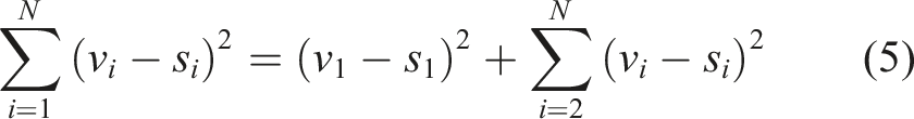
Further, we know that party i = 1 must win all of the seats, such that s₁ = 1. We also know, therefore, that all other parties must not win any seats at all, such that s_i≠1 = 0. This gives:

{(v_{1} - 1)}^{2} + \sum_{i = 2}^{N} {(v_{i} - 0)}^{2}

(6)

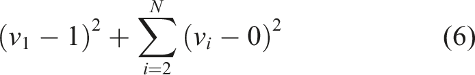
After expanding out the brackets and simplifying, the equation reduces to:

1 - 2 v_{1} + \sum_{i = 1}^{N} v_{i}^{2}

(7)

And, by the definition of the effective number of vote-winning parties, shown in equation (4), we know that

\sum_{i = 1}^{N} v_{i}^{2} = 1 / N_{V}

, which we can substitute to get:

1 - 2 v_{1} + \frac{1}{N_{V}}

(8)

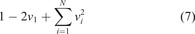
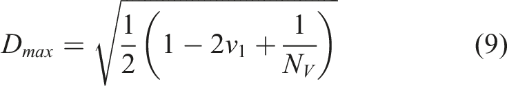
By substituting this for the sum in equation (3), we arrive at an upper bound on the Gallagher index for any party system of a fixed size, N_V, with a smallest vote share, v₁:

D_{\max} = \sqrt{\frac{1}{2} (1 - 2 v_{1} + \frac{1}{N_{V}})}

(9)

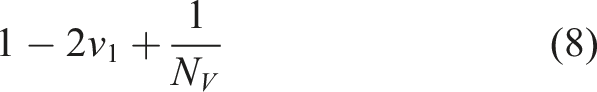
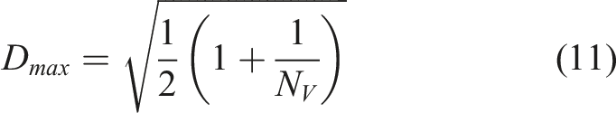
This then implies that, in the most disproportional case, where v₁ = 0, the upper bound on the Gallagher index for any party system with N_V effective vote-winning parties must be:

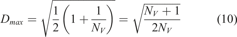
D_{\max} = \sqrt{\frac{1}{2} (1 + \frac{1}{N_{V}})} = \sqrt{\frac{N_{V} + 1}{2 N_{V}}}

(10)

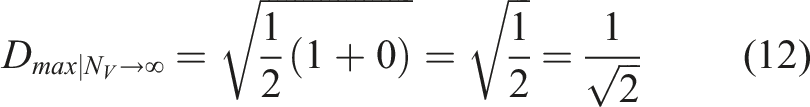
Figure 1 shows how this upper bound changes as the effective number of vote-winning parties increases. As N_V grows, the ceiling on the Gallagher index shrinks, reducing the possible range of disproportionality scores. The bound then converges on $1 / \sqrt{2}$ , which occurs in the limiting case where N_V → ∞. To see how, recall from equation (10) that:

D_{\max} = \sqrt{\frac{1}{2} (1 + \frac{1}{N_{V}})}

(11)

Figure 1.

Where the effective number of vote-winning parties tends to ∞, the upper bound on the Gallagher index tends to 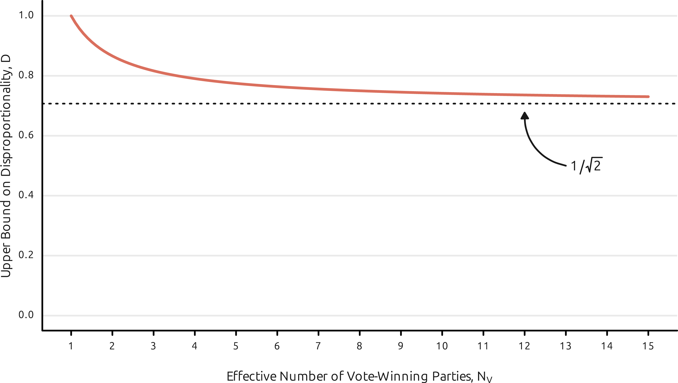$1 / \sqrt{2}$ . As such, the Gallagher index is constrained by the size of the party system.

So, as N_V tends to ∞, 1/N_V tends towards 0, giving:¹

D_{m a x | N_{V} \to \infty} = \sqrt{\frac{1}{2} (1 + 0)} = \sqrt{\frac{1}{2}} = \frac{1}{\sqrt{2}}

(12)

Holding the party system’s size constant

We have seen that the size of the party system bounds the range of values that the Gallagher index can take. Thus, apparent changes in disproportionality could, in certain circumstances, arise due to changes in party-system fragmentation. This quality reflects a real aspect of disproportionality, but will not always be desirable (e.g. where one would like to compare only the structural features of electoral systems). As such, it may sometimes be useful to hold the impact of the party system’s size constant. To this end, we can normalise the Gallagher index to ensure that it always outputs values from 0 (perfect proportionality) to 1 (maximal disproportionality), no matter the effective number of vote-winning parties. To do this, we need only divide equation (3) by equation (10), giving:

D_{norm} = \sqrt{\frac{\frac{1}{2} \sum_{i = 1}^{N} {(v_{i} - s_{i})}^{2}}{\frac{N_{V} + 1}{2 N_{V}}}}

(13)

Simplifying the fraction inside this equation then gives:

\frac{\frac{1}{2}}{\frac{N_{V} + 1}{2 N_{V}}} = \frac{1}{2} \times \frac{2 N_{V}}{N_{V} + 1} = \frac{N_{V}}{N_{V} + 1}

(14)

This allows us to write the normalised index as follows:

D_{norm} = \sqrt{\frac{N_{V}}{N_{V} + 1} \sum_{i = 1}^{N} {(v_{i} - s_{i})}^{2}}

(15)

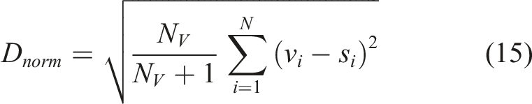
Figure 2 shows the distribution of disproportionality scores from 47,125 district-level contests in ‘simple electoral systems’—single-tier elections using first-past-the-post or districted party list proportional representation (for a fuller description, see Shugart and Taagepera 2017)—at 647 elections in 120 countries between 1900 and 2024, taken from The Elections Archive (Kollman et al., 2025). As the left-hand panel makes clear, the normalised and unnormalised indexes tend to move in tandem. However, the unnormalised index, D, often varies for any given value on the normalised index, D_norm, evidencing the impact of the party system. Indeed, where D_norm = 0.5, D varies by around 0.125—one-eighth the scale’s possible range.

Figure 2.

Disproportionality across 47,125 electoral districts at 647 elections in 120 countries from the Constituency-Level Elections Archive. The Gallagher index, D, shows some variation at a given value of the normalised index, D_norm. Both indexes track the largest party’s vote–seat gap |v₁ - s₁|, though D_norm does so spanning the full range between 0 and 1.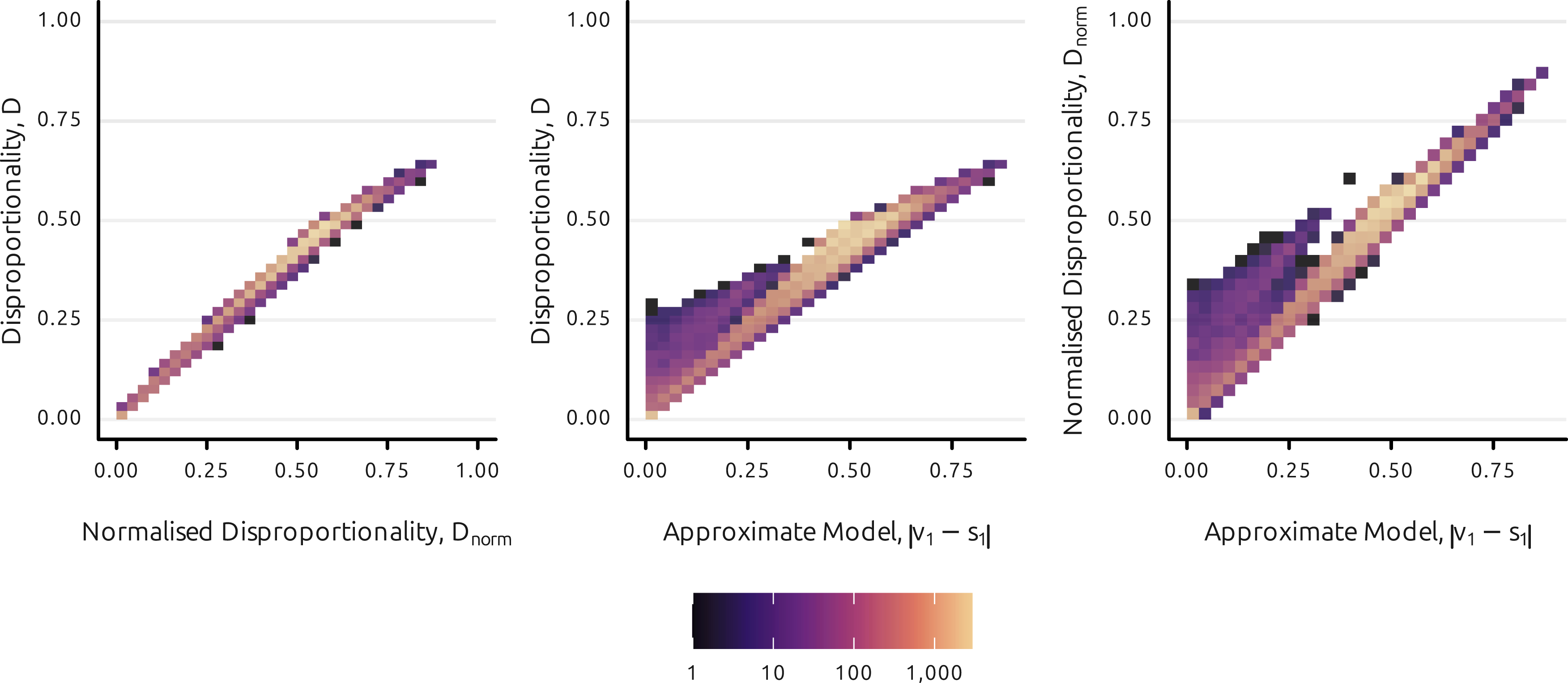

Given equations (3) and (15), we might expect the first-placed party to have the greatest impact on the disproportionality that we observe. Thus, following Shugart and Taagepera (2017), I predict both D and D_norm using a simple model where $\hat{D} = {\hat{D}}_{norm} = | v_{1} - s_{1} |$ . The middle and right-hand panels of Figure 2 plot D and D_norm against the model’s predictions and show very similar results. However, the right-hand panel also highlights an attractive feature of D_norm: its lower bound is |v₁ − s₁| rather than $1 / \sqrt{2} | v_{1} - s_{1} |$ , making prediction somewhat simpler.

Figure 3 uses data from ParlGov (Döring and Manow 2024) to plot values from each index at elections in the Netherlands, Ireland, and Australia: three countries that have experienced low, medium, and high disproportionality since the end of the Second World War. Due to the upper bound that I identify above, the normalised index produces larger values than the unnormalised one. However, the difference between the two also varies from case to case. In the Netherlands, the mean absolute error between the two indexes is negligible (MAE = 0.006). But in Ireland (MAE = 0.01) and Australia (MAE = 0.02) these differences are somewhat more pronounced. Indeed, in the latter case, the gap between the two measures grows to 0.05 at the most recent election. To put this figure in perspective, the Gallagher index, D, has a standard deviation of 0.07 across all legislative elections in the ParlGov data. Clearly, the impact of party system size is not trivial: in the Australian case, the difference between D and D_norm represents a 0.7 standard deviation difference in the value of the unnormalised index.

Figure 3.

Disproportionality in three countries—the Netherlands, Ireland, and Australia—that exhibit high, medium, and low levels of disproportionality at legislative elections. Note that the difference between the Gallagher index, D, and the normalised index, D_norm grows as both indexes increase. Data here come from ParlGov.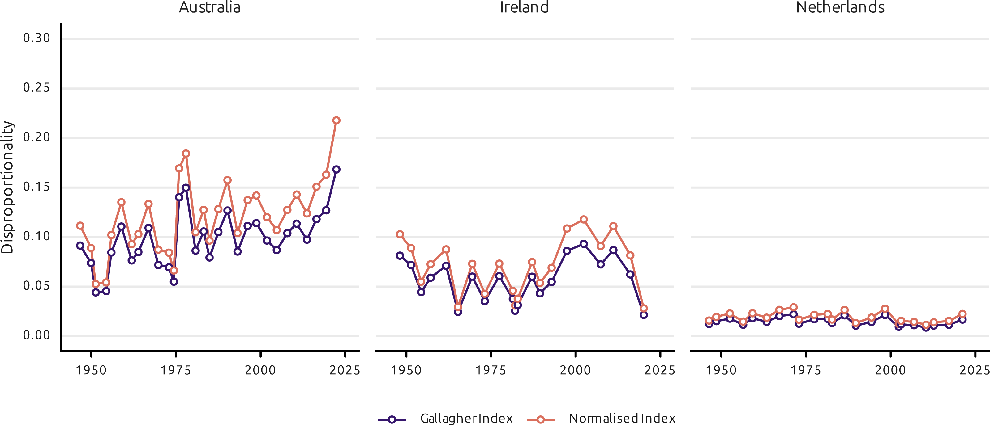

Which index to use depends on the question at hand. The bound that I identify above makes clear that fragmentation is inherent to disproportionality. As such, the unnormalised index will be appropriate whenever fragmentation is part of the theory of interest. For instance, when studying countries like Britain, where the party system has undergone considerable fragmentation (Prosser, 2024), it may be more appropriate to use the unnormalised index since this fragmentation may have made a meaningful contribution to electoral disproportionality. By contrast, the normalised index measures how the disproportionality observed compares to the maximum level possible given the effective number of vote-winning parties. Thus, research that looks to compare only structural features of the electoral system, such disproportionality attributable to the seat allocation model holding other factors constant, might prefer to use this version instead. More generally, the normalised index complements rather than replaces the Gallagher index: the former asks how disproportional an election was relative to its feasible maximum, while the latter asks how disproportional it was overall.

Conclusion

Though political scientists often assume that the Gallagher index varies between 0 (perfect proportionality) and 1 (perfect disproportionality), I show that this is almost never the case. Instead, I prove that the size of the party system as measured in effective vote-winning parties, N_V, constrains the index from above such that it can reach a maximum of $\sqrt{(N_{V} + 1) / 2 N_{V}}$ . I then propose a new normalised index that falls between 0 and 1 no matter the size of the party system.

My findings have implications for measurement, data management, and normative theory. On measurement, the normalised index that I propose provides a complement to the Gallagher index that removes variation caused by party-system fragmentation. On data management, the upper bound that I identify suggests that any values of the Gallagher index that exceed $\sqrt{(N_{V} + 1) / 2 N_{V}}$ can be flagged as probable errors. On normative theory, researchers and practitioners may find the normalised index useful when setting benchmarks for “acceptable” levels of disproportionality, since it provides a reference that does not vary according to how many parties are competing in elections. As such, the contributions that I make not only clarify the mathematical properties of a popular index in political science but also offer tools to improve the quality of our democracies.

However, my findings also suggest that more work needs to be done both to conceptualise what disproportionality really means and how it should best be measured. There is good reason to sympathise with Goldenberg and Fisher (2019), Van Puyenbroeck (2008), and others who argue persuasively in favour of alternative relative measures like the one first proposed by Sainte-Laguë (1910). As well as satisfying Dalton’s principle of transfers, the Sainte-Laguë index is unaffected by party-system fragmentation and, most importantly, puts the voter first.

Footnotes

ORCID iD

Jack Bailey

Funding

The author received no financial support for the research, authorship, and/or publication of this article.

Declaration of conflicting interests

The author declared no potential conflicts of interest with respect to the research, authorship, and/or publication of this article.

Note

Author biography

Jack Bailey is a Lecturer in Quantitative Political Science at the University of Manchester and Co-Director of the British Election Study.

References

Amore

Corina

(2021) Political elections and corporate investment: international evidence. Journal of International Business Studies 52(9): 1775–1796. https://doi.org/10.1057/s41267-021-00421-6

Anckar

(1997) Determinants of disproportionality and wasted votes. Electoral Studies 16(4): 501–515. https://doi.org/10.1016/S0261-3794(97)00038-3

Dahl

(1971) Polyarchy: Participation and Opposition. Yale University Press.

Dalton

(1920) The measurement of the inequality of incomes. The Economic Journal 30(119): 348. https://doi.org/10.2307/2223525

Döring

Manow

(2024) Parliaments and governments database (ParlGov). Harvard Dataverse. Available at: https://doi.org/10.7910/DVN/2VZ5ZC

Duverger

(ed) (1964) Political Parties: Their Organization and Activity in the Modern State. Methuen. University Paperbacks 82.

Gallagher

(1991) Proportionality, disproportionality and electoral systems. Electoral Studies 10(1): 33–51. https://doi.org/10.1016/0261-3794(91)90004-C

Goldenberg

Fisher

(2019) The Sainte-Laguë index of disproportionality and Dalton’s principle of transfers. Party Politics 25(2): 203–207. https://doi.org/10.1177/1354068817703020

Katz

(1980). A Theory of Parties and Electoral Systems. Johns Hopkins University Press. https://doi.org/10.1353/book.3506

10.

Kollman

Hicken

Caramani

, et al. (2025) The elections archive. Ann Arbor, MI: Center for Political Studies, University of Michigan.

11.

Laakso

Taagepera

(1979) Effective’ number of parties: a measure with application to West Europe. Comparative Political Studies 12(1): 3–27. https://doi.org/10.1177/001041407901200101

12.

Liberal Party of Canada (2016) Real Change: A Fair and Open Government. Liberal Party of Canada.

13.

Lijphart

(1994) Electoral Systems and Party Systems: A Study of Twenty-Seven Democracies, 1945–1990. Oxford University Press.

14.

Lijphart

(2012) Patterns of Democracy: Government Forms and Performance in Thirty-Six Countries. 2nd edition. New Haven, CT: Yale University Press.

15.

Loosemore

Hanby

(1971) The theoretical limits of maximum distortion: some analytic expressions for electoral systems. British Journal of Political Science 1(4): 467–477. https://doi.org/10.1017/S000712340000925X

16.

Matakos

Savolainen

Troumpounis

, et al. (2024) Electoral institutions and intraparty cohesion. Journal of Political Economy Microeconomics 2(4): 883–916. https://doi.org/10.1086/731286

17.

McGann

. (2006). The Logic of Democracy: Reconciling Equality, Deliberation, and Minority Protection. University of Michigan Press.

18.

Norris

(2024) Things fall apart, the center cannot hold’: fractionalized and polarized party systems in Western democracies. European Political Science 23(4): 546–566. https://doi.org/10.1057/s41304-023-00467-0

19.

Prosser

(2024) Fragmentation revisited: the UK general election of 2024. West European Politics 48(6): 1–13. https://doi.org/10.1080/01402382.2024.2430915

20.

Rae

(1971) The Political Consequences of Electoral Laws. Yale University Press. Political Science.

21.

Sainte-Laguë

(1910) La représentation proportionnelle et la méthode des moindres carrés. Annales scientifiques de l’École normale supérieure 27: 529–542. https://doi.org/10.24033/asens.627

22.

Shugart

Taagepera

. (2017). Votes from Seats: Logical Models of Electoral Systems. Cambridge University Press.

23.

Special Committee on Electoral Reform (2016) Strengthening Democracy in Canada: Principles, Process and Public Engagement for Electoral Reform. House of Commons, Vol. 3.

24.

Taagepera

Grofman

(2003) Mapping the indices of seats–votes disproportionality and inter-election volatility. Party Politics 9(6): 659–677. https://doi.org/10.1177/13540688030096001

25.

Toshkov

Mazepus

(2023) Does the election winner–loser gap extend to subjective health and well-being? Political Studies Review 21(4): 783–800. https://doi.org/10.1177/14789299221124735

26.

Valentim

Dinas

(2024) Does party-system fragmentation affect the quality of democracy? British Journal of Political Science 54(1): 152–178. https://doi.org/10.1017/s0007123423000157

27.

Van Puyenbroeck

(2008) Proportional representation, gini coefficients, and the principle of transfers. Journal of Theoretical Politics 20(4): 498–526. https://doi.org/10.1177/0951629808093778