Sage Journals: Discover world-class research

Abstract

Background:

With many disease-modifying therapies currently approved for the management of multiple sclerosis, there is a growing need to evaluate the comparative effectiveness and safety of those therapies from real-world data sources. Propensity score methods have recently gained popularity in multiple sclerosis research to generate real-world evidence. Recent evidence suggests, however, that the conduct and reporting of propensity score analyses are often suboptimal in multiple sclerosis studies.

Objectives:

To provide practical guidance to clinicians and researchers on the use of propensity score methods within the context of multiple sclerosis research.

Methods:

We summarize recommendations on the use of propensity score matching and weighting based on the current methodological literature, and provide examples of good practice.

Results:

Step-by-step recommendations are presented, starting with covariate selection and propensity score estimation, followed by guidance on the assessment of covariate balance and implementation of propensity score matching and weighting. Finally, we focus on treatment effect estimation and sensitivity analyses.

Conclusion:

This comprehensive set of recommendations highlights key elements that require careful attention when using propensity score methods.

Keywords

Comparative effectiveness covariate selection inverse probability of treatment weighting observational study propensity score matching real-world data

Introduction

Multiple sclerosis (MS) is a chronic disease of the central nervous system, without any known cure. As many disease-modifying therapies (DMTs) are currently available for the management of MS, there is a growing need to evaluate the comparative effectiveness and safety of those DMTs. Real-world data (RWD) sources, such as disease registries (e.g. MSBase and NeuroTransData), electronic medical records, and administrative claims databases, have increasingly been recognized as an essential part of evidence-based research in the MS literature, partly due to their ability to provide larger cohorts and longer follow-up and to capture various factors related to disease progression in clinical practice settings.^1,2 Specific opportunities and challenges to each type of data source have previously been described in the context of MS,³ and thorough reports of currently available MS registries, covering over 500,000 MS patients, have recently been published.^2,4

RWD offer great opportunities for comparative effectiveness research but are associated with specific challenges. In particular, confounding occurs when patient characteristics at study entry (i.e. baseline) affect both the probability of receiving the treatment and the outcome. As a result, differences in the outcome between treated and control patients may be partially attributable to differences in the distribution of their confounders rather than to the treatment itself. Propensity score (PS) methods have rapidly gained popularity as a confounding adjustment approach among clinical researchers in MS (Figure 1), with matching or weighting of study participants being the most commonly used methods in the field.⁵ In parallel, PS approaches have undergone significant methodological advances, making it difficult for practitioners and end-users to keep up with the fast pace of new information.

Figure 1.

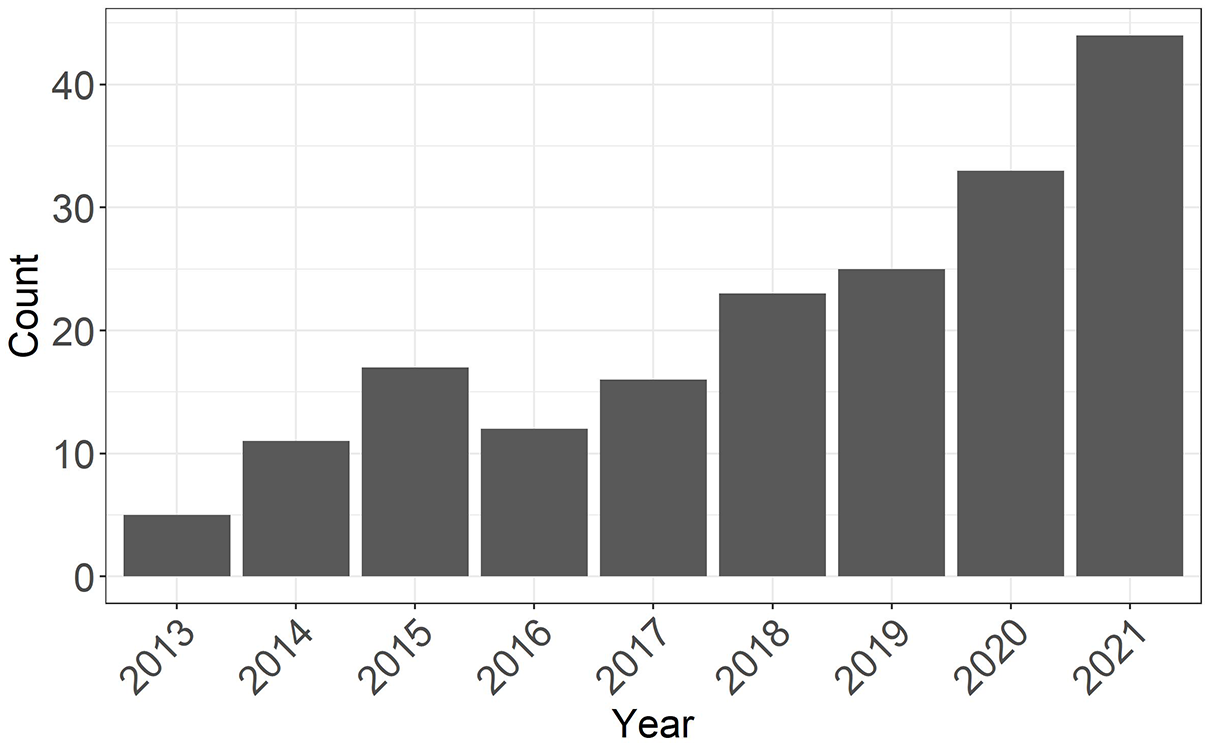
Number of publications by year identified on PubMed with the search query (multiple sclerosis) and (propensity score).

To provide reliable real-world evidence, it is critical that PS approaches are correctly implemented and adequately reported.⁶ Unfortunately, the quality of reporting and implementation of PS methods in MS studies is often suboptimal.⁵ Improvements in the application and reporting of propensity score analyses are urgently needed to enhance the reproducibility and generalizability of research findings. This article, targeted to MS clinicians and researchers, therefore aims to offer exhaustive practical guidance on the implementation of PS matching and weighting for comparing the relative effectiveness of two treatments. A comprehensive review of PS methods is beyond the scope of this paper and has already been provided in the broader context of neurology.⁷

Basic principles of propensity scores

The PS is the patient’s probability of receiving the treatment versus control (e.g. standard of care or active comparator) given a sufficient set of individual characteristics at baseline (before or at the time of cohort entry, before treatment initiation). In randomized controlled trials, the true PS is known by design. In contrast, the PS is unknown in RWD because treatment selection is not randomized and may depend on several factors such as characteristics of the patient and preferences of their treating physician. Therefore, it should be estimated from the observed data of the patient and their clinical environment.

A PS analysis leverages the balancing property of the PS to control for confounding in RWD.⁸ The balancing property means that the distribution of measured covariates between the treatment and control group is expected to be similar for neighboring PS values. For example, we can choose patients from the treatment and control groups with similar estimated PS values (say, estimated PS values close to 0.75). These patients are expected to have similar values for baseline covariates, and thus may be considered comparable. Then, on average, differences in outcomes between treated and control patients can only be attributed to differences in treatment, provided that all confounders have been measured and used to estimate the PS. While randomization in clinical trials ensures that, on average, patients in the treatment and control groups are comparable with respect to both measured and unmeasured confounders,⁹ the estimated PS in RWD ensures comparability with respect to measured confounders only.

Methods that use the PS to control for confounding, like any approach that attempts to estimate causal effects, must meet four conditions to allow estimation of the causal effect: no unmeasured confounding, positivity, consistency, and no interference.^8,10 These conditions are explained and illustrated in Table 1. In MS, the positivity condition, which requires every patient to be eligible to receive either treatments given their baseline characteristics, can easily be violated. This situation typically arises when DMTs are marketed at different dates or when they have different contraindications. For example, imagine a study comparing natalizulimab (marketed in 2006) to ocrelizumab (marketed in 2017) in the United States between 2010 and 2020. Patients who started natalizumab prior to 2017 were not eligible to receive ocrelizumab. Consequently, a PS analysis will violate the positivity condition because calendar year affects MS patient care, prognosis, and outcomes, thus acting as a confounder. Restricting the study period to patients who started either treatment when both were available on the market may resolve this structural positivity violation.

Table 1.

A brief explanation of conditions required for the use of propensity score methods.

Condition	Description	Example
No unmeasured confounding	All confounders must be measured in the data source. If two confounders are strongly correlated, it is sufficient to measure only one of them (exchangeability). This condition cannot be verified in practice, but sensitivity analyses can quantify the impact of violations	The number of gadolinium-enhancing lesions may be a confounder in the treatment–outcome relationship of interest, yet the data source for the study (e.g. a claims database) does not capture it. Then, the condition of no unmeasured confounding is violated
Positivity	Each patient should a priori be eligible for both treatments. Positivity violations may be deterministic (e.g. the patient with comorbidity is not eligible to receive the treatment) or random (e.g. the patient is eligible, but the sample was too small to capture that aspect). This condition may be verified empirically	In a study comparing the effectiveness of two DMTs, the study period should be restricted to the time period when both drugs were available to patients for positivity to be satisfied
Consistency	Also known as “well-defined treatment” or “no multiple versions of treatment.” This condition requires that there be only one version of the treatment. When multiple versions of the treatment exist (e.g. different doses), disease area expert consensus should inform whether considering the different versions as the same treatment is warranted	Patients receiving either a low- or high-dose interferon beta-1 may be grouped into one treatment arm. For consistency to hold, the effect of low- or high-dose interferon beta-1 on the outcome should be the same
No interference	This condition requires that a patient’s outcome is not influenced by other patients’ treatment assignments. For example, this condition is violated when the outcome is an infectious disease, where treating an individual may protect others from infection. In MS, this condition likely holds, although available data rarely allow its plausibility to be assessed	If a participant is prescribed a DMT, and his spouse is not (while both are in a study), but they share the medication, then this condition is violated

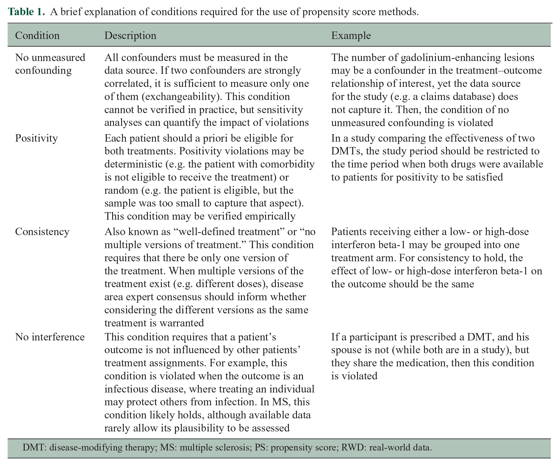
DMT: disease-modifying therapy; MS: multiple sclerosis; PS: propensity score; RWD: real-world data.

Recommendations for the implementation of propensity score matching and weighting

In the next sections, we give a step-by-step procedure to apply PS matching and weighting, starting from the selection of covariates to include in the PS model and ending with specific considerations for sensitivity analyses. Based on evidence gathered from the published biostatistics and epidemiology literature, we summarize recommendations on how best to conduct each step, where possible. Guidelines for reporting a PS analysis are summarized in Table 2, and examples of good practice in a few, targeted studies in other disease areas are described in Supplemental Table 1. We provide example R code to reproduce the main steps of the analysis in the Supplemental Material, section 2.

Table 2.

Summary of recommendations on the reporting of propensity score methods in multiple sclerosis research.

Manuscript section	Proposed items to report
Abstract	1. Indicate target estimand (e.g. ATE, ATT) 2. Indicate PS approach used and provide brief summary specific to the approach (e.g. provide matching ratio and sampling method used if using PS matching)
Introduction	1. State research question 2. Indicate choice of the target population and target estimand in relation to the research question
Methods	Covariate selection for PS model 1. Indicate method used for selecting covariates (e.g. empirical knowledge) 2. List covariates (and proxy variables) used for PS estimation and how they were handled in the analysis (e.g. categories, interactions, polynomial terms, splines) PS estimation 3. Indicate method used for PS estimation (e.g. logistic regression) 4. Indicate how missing data and sparsity was addressed in PS estimation (if relevant) PS method used 5. State type of PS method used (matching, weighting) 6. If PS matching: provide details of matching algorithm such as type of matching (e.g. nearest neighbor), matching ratio, caliper width, sampling with/without replacement, statistical method for the analysis of matched data 7. If PS weighting: Specify the type of weights (e.g. stabilized) and whether weights were applied throughout or as subgroup-specific weights (if heterogeneity present), statistical method used for variance estimation, method used for truncation (if applicable) Balance assessment and PS diagnostics 8. Indicate balance measure and threshold (e.g. absolute SMD, <0.1) and overlap assessment methods 9. For PS weighting: Report distribution of unstabilized and stabilized weights (mean, max, min, range, if applicable) and whether weights were truncated (if applicable) Estimation of treatment effect and standard errors 10. Report model used to estimate treatment effect and the standard error (e.g. bootstrapping, cluster-robust standard error) 11. List covariates included in outcome model (if applicable) Other 12. Indicate how PS conditions were verified and, when possible, if they were met 13. Indicate how adherence was handled 14. Describe additional analyses (subgroup, sensitivity) 15. Report software packages used
Results	1. Report sample size at each stage (eligible, included, analyzed) 2. For each treatment group, provide number of patients, distribution of baseline characteristics (including missing data), and SMDs for all covariates before and after matching/weighting 3. Report any covariate imbalances and whether additional adjustments were made 4. Provide numerical and/or graphical representation of PS distribution (e.g. histogram) 5. Report crude and the adjusted point estimate of the treatment effect and associated measure of variability
Discussion	1. Interpret effect estimate in relation with research question, choice of PS approach, target population and estimand 2. Explain how potential unmeasured confounding was addressed 3. Provide a justification of PS conditions in the current research context
Appendix	1. Provide results from additional analyses (subgroup, interactions or effect modifications, sensitivity analyses). 2. Provide more details of PS approach if needed (e.g. diagnostics, HdPS algorithm)

ATE: average treatment effect; ATT: average treatment effect in the treated; HdPS: high-dimensional propensity score; PS: propensity score; SMD: standardized mean difference.

Covariate selection

Covariates included in a PS model must be selected to restore balance in the covariate distribution of treated and control patients. Enough covariates must be included to achieve this goal, and thus to control for confounding. The general consensus on covariate selection for the PS is to rely on expert knowledge in relevant disease areas to better capture the relationship among covariates, treatment, and outcome (see Supplemental Table 2).¹¹ Covariates that are confounders or risk factors for the outcome should be included in the PS model.¹² Inclusion of covariates that are only predictors of treatment but not associated with the outcome should be avoided as their inclusion tends to increase the variance of the treatment effect estimates.^12,13 Importantly, covariates included in the PS model must be captured at baseline; adjusting for covariates which are measured after baseline is strongly discouraged because such covariates may be affected by the treatment.¹⁴

In MS, a recent review found that an average of eight covariates (range: 3–16) were selected to construct the PS, with the following baseline covariates most frequently used: age, sex, disease duration, number of relapses in the 12 months prior to baseline, Expanded Disability Status Scale (EDSS) score at baseline, and previous treatments.⁵ However, only 21% of the reviewed studies reported how the list of covariates was determined.⁵

A practical issue with covariate selection for the PS is that relevant confounders are sometimes unavailable in the data source, which violates the condition of no unmeasured confounding. We provide examples and discuss mitigation strategies in the Supplemental Material, section 2.

Data-driven covariate selection approaches, such as statistical tests or automated machine learning approaches (e.g. forward or backward selection, LASSO), are often used in the medical literature. Caution is advised when using these methods because some are designed to select covariates that optimize the prediction of treatment assignment, which may lead to the exclusion of important covariates (e.g. risk factors), threaten the positivity condition, and lead to poor covariate overlap (see section “Assessment of overlap and positivity”).^12,15

Estimation of the propensity score

Once a set of covariates is selected, different modeling approaches can be used to arrive at the final PS model, with the overarching goal of achieving covariate balance after PS matching or weighting (see section “Assessment of balance”). Logistic regression is the most popular approach among researchers in MS.⁵ Kainz et al.¹⁶ recommend an iterative procedure to guide the construction of the PS model. First, all selected covariates should be included as main effects in the regression model, along with biologically plausible nonlinear (e.g. polynomial or splines) and interaction terms. Second, if balance is not achieved for a given covariate based on the initial model, consider adding nonlinear or interaction terms for that covariate. Finally, repeat the first and second steps until the balance is achieved on all covariates, if possible (see section “Treatment effect estimation and interpretation” for recommendations when the balance is not achieved). The final model should be reported clearly, with all interaction and non-linear terms detailed, and whether and how covariates were transformed. Such details were seldom explicitly reported in MS studies.⁵

Logistic regression requires the PS model to be correctly specified (i.e. the appropriate covariate transformations, nonlinear terms, and interaction terms are included) for the estimated PS to possess the balancing property.⁸ In practice, this requirement is often unrealistic. Alternatively, flexible modeling approaches such as machine learning methods and splines remain agnostic to the specification of the PS model and instead focus on finding the most accurate predictions for the PS.¹⁷ However, such methods may deteriorate covariate balance and overlap if these properties are not considered during the estimation of the PS model.¹⁸ The use of flexible modeling methods to estimate the PS in MS remains limited; none of the 39 papers included in a recent review on the use of PS methods in MS reported using such methods.⁵

Goodness-of-fit tests (“how well the model describes the data”) such as the Hosmer–Lemeshow test statistic and model discrimination measures (“how well the model differentiates between patients with or without the outcome”) such as the c-statistic should not be used to guide variable selection, evaluate whether the PS model has been correctly specified, or detect unmeasured confounding.^19–21 These measures assess the prediction accuracy and model fit of the PS model while the goal of the PS is to achieve covariate balance. Hence, the adequacy of the fitted PS model should be evaluated accordingly with balance assessment metrics (see section “Assessment of overlap and positivity”).

Assessment of overlap and positivity

PS overlap refers to the range of estimated PSs covered by both treatment groups. High overlap is desirable because it indicates that treated and control patients are more comparable, thus warranting a comparison between the two treatments with a PS analysis. PS overlap is assessed by inspecting the distributions of the estimated PSs between the treated and control groups with visual (e.g. side-by-side boxplots and mirrored histograms) and numerical tools (summary statistics of the estimated PS by treatment group).^20,22 An example of mirrored histograms is shown in Figure 2 using a simulated data set. Trimming (i.e. excluding patients in) the regions of non-overlap can be performed. However, if a large portion of the original sample is removed after trimming, the study population might change and, as a consequence, differ from the original target population.²³ This might also suggest an insufficient overlap between the two treatments, which can be a sign that the two treatments are used in different populations and that the comparative effectiveness question is not relevant.²⁴

Figure 2.

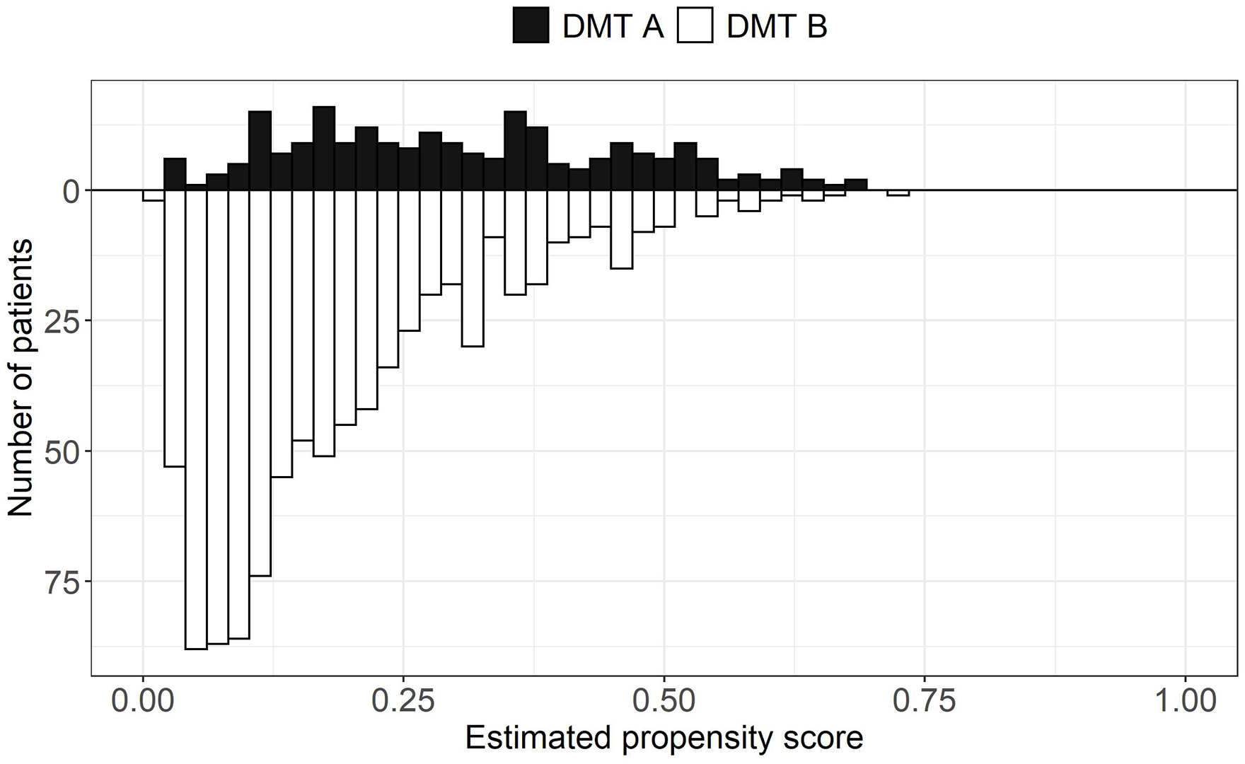
Mirrored histograms showing the distributions of the estimated propensity scores by hypothetical treatment groups (DMT A vs DMT B). The distributions show good overlap. The data presented in this figure are based on a simulated data set.

The positivity condition can be examined empirically with the estimated PSs and the visual and numerical tools described above. Poor overlap or estimated PSs too close to 0 or 1 both indicate a potential positivity violation, suggesting that some patients would not have been eligible to receive the alternative treatment. Additional verification steps should be taken, for example, by inspecting the covariates of patients with extreme estimated PSs or in the non-overlapping region(s) to understand which factors led to such findings. Covariates can also be tabulated by the treatment group to identify random positivity violations.²⁵

Assessment of balance

Standardized mean differences (SMDs) are the most popular numerical summaries of covariate balance in MS.⁵ They are the preferred measure to compare proportions or means of a covariate between treatment groups because they are not influenced by measurement scale or sample size. Performing numerical and visual checks with SMDs before and after matching, or in the unweighted and weighted samples in the case of PS weighting, is generally recommended; Figure 3 shows an example of a Love plot, which provides a concise prematching and postmatching (or weighting) balance summary for all covariates.²⁶ A threshold should be defined a priori to classify a covariate as adequately balanced. Although there is no universally accepted threshold, the value of 0.1 is often used in practice, where an SMD (in absolute value) below 0.1 indicates sufficient balance on the covariate.²⁰ To some extent, the threshold for acceptable balance depends on the prognostic importance of the confounders; less stringent thresholds may be appropriate for covariates weakly associated with the outcome while more stringent thresholds may be used for important ones.²² Balance should also be assessed for the entire distribution of the covariate and not merely for means or proportions (see Supplemental Material, section 3). MS researchers should employ a range of complementary visual and numerical diagnostics as opposed to relying on a single one.^20,27

Figure 3.

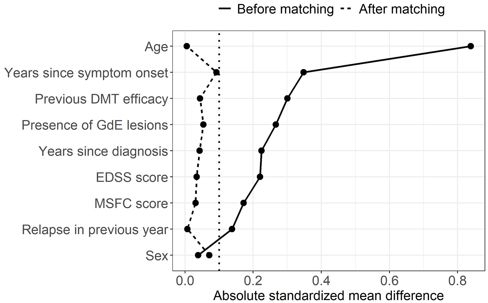
Love plot with absolute standardized mean differences between two hypothetical treatment groups (DMT A vs DMT B) for a subset of covariates before and after matching. The vertical dotted line represents the threshold of 0.1 under which balance is considered acceptable. The data presented in this figure are based on a simulated data set.

Assessment of balance should not be conducted with statistical tests (e.g. t-test, McNemar tests, and Wilcoxon rank test) because these are affected by sample size. For example, nonsignificant differences between treatment groups after matching may be due only to a reduced sample size after discarding unmatched patients. More fundamentally, statistical tests make inference on balance at the population level, which is inappropriate because a balance must rather be achieved in the sample.^14,28

Researchers should check the balance for all covariates, including those not included in the PS model.²² If imbalances are observed in some of the covariates that were not initially selected to estimate the PS, researchers should reassess whether they are important covariates and, if so, include them in the PS model. If imbalances remain despite efforts to improve the PS model through the iterative model building procedure, strategies can be adopted at the treatment effect estimation step (see section “Treatment effect estimation and interpretation”). However, this might also be a sign that the data are not suitable to answer the comparative effectiveness research question.²²

Implementation of matching

PS matching involves forming matched sets of treated and control patients with a similar value of the estimated PS. The intent is to mimic treatment randomization, to allow estimation of the treatment effect by direct comparison of outcomes within matched sets. The implementation of matching implies choosing an appropriate algorithm to form the matched sets (see Austin²⁹ for a description of matching algorithms). This entails decisions on several factors: what is the target population, how to define the closeness of matched patients, whether matching should be performed with or without replacement, and how many control patients should be matched to each treated patient. To some extent, the choices depend on the characteristics of the available data.

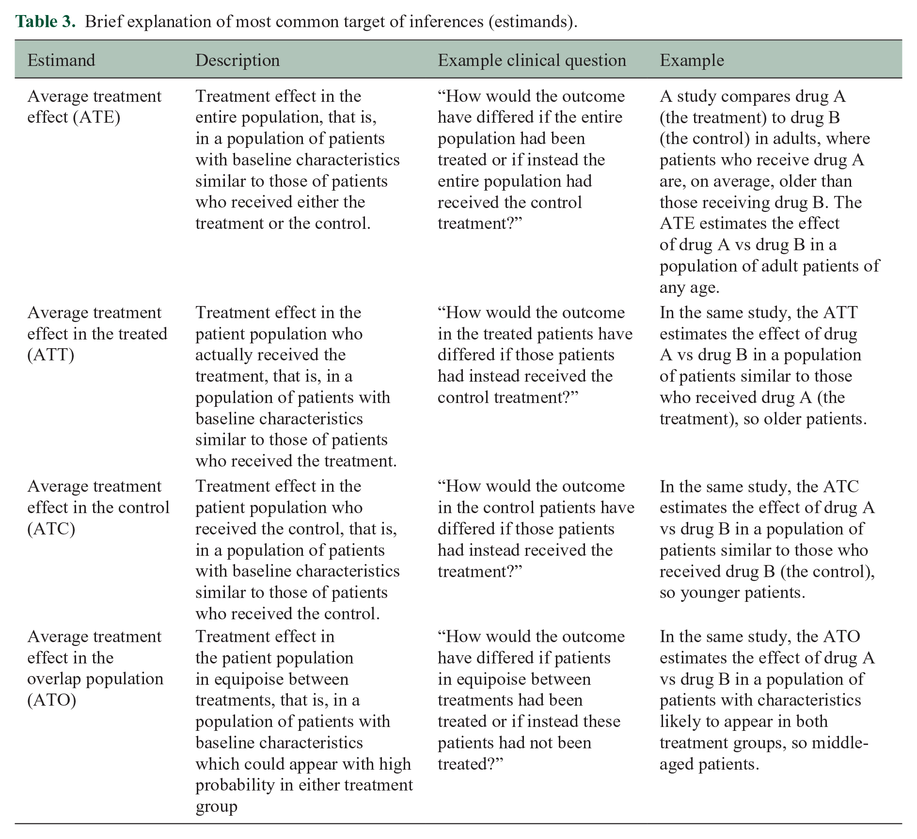
The choice of the matching algorithm must be aligned with the target estimand (Table 3).³⁰ This is crucial because treatment effect estimates may generalize to different target populations and thus the target estimands will differ, especially if the distribution of the PS and covariates differ between the two treatment groups.³¹ Most applications of matching match control patients to treated patients and thus estimate the average treatment effect in the treated (ATT). If instead, treated patients are matched to control patients, the target estimand becomes the average treatment effect in the controls (ATC). Full matching successively matches controls to treated patients, and vice versa, thus targeting the average treatment effect (ATE).

Table 3.

Brief explanation of most common target of inferences (estimands).

Estimand	Description	Example clinical question	Example
Average treatment effect (ATE)	Treatment effect in the entire population, that is, in a population of patients with baseline characteristics similar to those of patients who received either the treatment or the control.	“How would the outcome have differed if the entire population had been treated or if instead the entire population had received the control treatment?”	A study compares drug A (the treatment) to drug B (the control) in adults, where patients who receive drug A are, on average, older than those receiving drug B. The ATE estimates the effect of drug A vs drug B in a population of adult patients of any age.
Average treatment effect in the treated (ATT)	Treatment effect in the patient population who actually received the treatment, that is, in a population of patients with baseline characteristics similar to those of patients who received the treatment.	“How would the outcome in the treated patients have differed if those patients had instead received the control treatment?”	In the same study, the ATT estimates the effect of drug A vs drug B in a population of patients similar to those who received drug A (the treatment), so older patients.
Average treatment effect in the control (ATC)	Treatment effect in the patient population who received the control, that is, in a population of patients with baseline characteristics similar to those of patients who received the control.	“How would the outcome in the control patients have differed if those patients had instead received the treatment?”	In the same study, the ATC estimates the effect of drug A vs drug B in a population of patients similar to those who received drug B (the control), so younger patients.
Average treatment effect in the overlap population (ATO)	Treatment effect in the patient population in equipoise between treatments, that is, in a population of patients with baseline characteristics which could appear with high probability in either treatment group	“How would the outcome have differed if patients in equipoise between treatments had been treated or if instead these patients had not been treated?”	In the same study, the ATO estimates the effect of drug A vs drug B in a population of patients with characteristics likely to appear in both treatment groups, so middle-aged patients.

Matching patients requires a choice of a metric to quantify the similarity of patients within a matched set. Austin³² recommends matching based on the difference between the estimated PSs in the treated and control patients on the logit scale up to a fixed distance (i.e. caliper). The use of a caliper is encouraged to ensure better comparability between treatment groups in the matched sample. Smaller calipers will result in more homogeneous matched sets (reduced bias) but may also reduce the number of matched sets (increased variance).³³ Although there is no universally accepted caliper width, Austin³² recommends using 0.2 standard deviation of the logit of the estimated PSs.

Matching without replacement is most commonly used in the MS literature.⁵ In the context of matching controls to treated patients, matching with replacement can decrease bias because controls who are similar to more than one treated patient can be used multiple times.^22,28 It is especially helpful in situations when there are more treated patients than controls,²⁸ but it affects the estimation of the standard error of the treatment effect (see section “Estimation of standard error”). When matching with replacement, the number of times each control is used as a match should be inspected to ensure that the treatment effect estimate is not based on only a small number of controls.²⁸ When there are at least twice as many control patients as treated patients, Austin²⁹ discourages matching with replacement because it results in treatment effect estimates with similar bias compared to matching without replacement, but with increased variability.

In MS, 1:1 (treated:control) matching is most commonly implemented.⁵ Alternatives, such as fixed or variable 1:k matching which respectively finds k or up to k control matches for each treated patient, have been studied in limited settings. In the context of fixed 1:k matching without replacement, Austin³⁴ found that increasing k increases the bias in the treatment effect estimator while decreasing its variance and recommended matching with a fixed ratio of 1:1 or 1:2. Rassen et al.³⁵ found that variable ratio matching without replacement can decrease the variance of the treatment effect estimates without substantially increasing bias. However, they focused on continuous outcomes in situations where the number of controls is greater than the number of treated patients. Wang et al.³⁶ instead argued that, in the context of binary outcomes, the modest reduction in variability from variable ratio matching should be weighed against the practical advantages and transparency of 1:1 matching. In particular, variable-ratio matching complicates the display of baseline characteristics and balance assessments in the matched sample when matched sets have different numbers of patients.^35,37

Regardless of the choice of matching algorithm, the matched sample should be described in terms of sample size (overall and by treatment group), percent reduction in sample size from the original sample (overall and by treatment group), number of matched sets formed, and number of patients in each matched set (when using 1:k or variable ratio matching). Baseline characteristics in the matched sample should be displayed in a table along with the characteristics of the sample prior to matching. This is because the characteristics of the target population may have changed after implementing matching if any patients (for the ATE) or treated/control patients (for the ATT/ATC) were discarded due to an inability to find suitable matches. Visual tools can also help the reader appreciate this change.²³

Implementation of weighting

PS weighting involves estimating weights based on the PS for each patient. The intent of PS weighting is to create an “artificial” population in which confounding is removed and outcomes can be directly compared. Careful consideration must be given to the choice of weights to reflect the targeted estimand (see Table 3).³⁰ The most common weights, which are described in Desai and Franklin,²⁴ include inverse probability of treatment weights, targeting either the ATE or ATT depending on their specification. Alternatively, the overlap weights could be used to target a population of high clinical interest, that is, individuals for whom the treatment choice is ambiguous.³⁸

Extreme estimated PSs (e.g. <0.05 or >0.95) can result in a large or small inverse probability of treatment weights and thereby distort the representativeness of patients with very high probability of receiving a given treatment.²⁴ This can increase the variability of the treatment effect estimate.³⁹ Stabilized weights can be used as a mitigation strategy (see appendices in previous studies^39,40). Truncation (i.e. setting the extreme estimated PSs to prespecified threshold values) is also used to address extreme weights, although this will reduce the variance of the treatment effect estimator at the cost of potentially increasing its bias.²⁴ If large weights are an issue, the general recommendation is to choose a more extreme threshold for truncation (e.g. choosing the first percentile of the estimated weights rather than the fifth percentile).²⁴ Alternatively, the overlap weights are less sensitive to extreme weights.³⁸ We note that overlap weighting is a recent technique and that the study of its statistical properties is a topic of active research.

Treatment effect estimation and interpretation

In the matched or weighted sample, the treatment effect can be estimated by direct comparison of the outcomes if balance was achieved on all observed covariates. The treatment effect can then be interpreted at the level of the target population as described in Table 3; that is, it has a marginal interpretation.

If some covariates remained unbalanced despite following the iterative procedure to model the PS, a common strategy to deal with the residual imbalance is to estimate the treatment effect by fitting a so-called outcome model, a regression model that further adjusts for some covariates. Ho et al.²² suggest including all or a subset of the covariates used to fit the PS model in the outcome model, while Nguyen et al.⁴¹ propose including only the unbalanced covariates, a procedure known as double-adjustment. Shinozaki and Nojima⁴² advise against adjusting for covariates not included in the PS model because this might reduce the covariate balance achieved by the PS adjustment and consequently lead to bias in the estimated treatment effect. A direct consequence of covariate adjustment in the outcome model is that the estimated treatment effect (partially) depends on the distribution of patient-level characteristics and can therefore no longer be interpreted at the level of the target population.⁴³ In a recent review, 9 of 28 MS studies that used PS matching for the comparative effectiveness of two treatments reported imbalances after matching, yet only one study took specific actions to address the imbalances (i.e. adjusting for the imbalanced covariates in the outcome model for the treatment effect).⁵

Estimation of standard error

Estimation of the standard error for the estimated treatment effect after PS matching or weighting requires special considerations. Ignoring these considerations may lead to biased standard error estimates, ultimately exposing the study to potentially erroneous conclusions.

For PS matching, the variability of the estimated treatment effect is affected by the correlation between outcomes of patients in a matched set because patients within a matched set are more likely to be similar compared to two unmatched patients.⁴⁴ When matching without replacement, this correlation can be accounted for with a cluster-robust standard error estimator which treats the matched sets as clusters. Such standard errors can be obtained from generalized estimating equations or generalized linear mixed models, or with analytic formulas (see Greifer⁴⁵ for implementations in R). Standard errors from the matched bootstrap, which resamples matched sets instead of resampling patients from the full sample, also perform adequately in some settings.^46,47 When matching with replacement, the standard error estimation must account for an additional source of correlation introduced into the data because control patients may appear more than once in the matched sample. Standard error estimation in this context remains an active area of research; a few cluster-robust standard error estimators which also account for the duplication of controls in the matched sample have been evaluated in different contexts, however, without any proving consistently superior.^48,49 Standard errors based on the bootstrap can also be considered because they appear to perform well in practice.^48,50 While Abadie and Imbens⁵¹ showed that the standard bootstrap is not generally valid for matching with replacement (i.e. may not produce asymptotically correct standard errors), their findings were limited to the simple context of matching on a single covariate. Others have found that this theoretical result has little practical implications when matching on the estimated PS,⁵⁰ warranting the use of the standard bootstrap with caution. The most effective implementation of bootstrapping (e.g. whether to resample patients in the original sample or matched pairs in the matched sample) in any particular context remains an open question.

For PS weighting, standard errors are affected by the fact that weights “duplicate” some patients, thus introducing correlation in the weighted sample akin to the correlation introduced by duplicated controls in matching with replacement. Moreover, the standard errors must account for the fact that the weights are estimated instead of known, fixed quantities. Robust (often called “sandwich”) standard error estimators can be used in this context,^52–54 with several implementations available in R.^55–57 However, a recent study found that robust standard error estimators may be inappropriate when used with inverse probability of treatment weights targeting the ATT, in which case estimators based on stacked estimating equations should be preferred.^54,58 The bootstrap provides an alternative to estimate standard errors, although it is more computationally intensive.^50,59

Role of sensitivity analyses

A PS analysis depends on several key conditions, some of which are difficult or even impossible to evaluate in practice. For this reason, it is recommended to explore whether treatment effect estimates are sensitive to changes in decisions made in the course of the PS analysis via sensitivity analyses.

Bias due to unmeasured confounding remains the main concern after a PS analysis. However, in MS, a recent review found that only 34% of studies using PS methods reported a sensitivity analysis for unmeasured confounding.⁵ Advanced sensitivity analysis methods for unmeasured confounding quantify how the estimated treatment effect may be affected by an unmeasured confounder under some assumptions. Some methods require explicit specification of the nature of the unmeasured confounding. For example, the method of Lin et al.⁶⁰ quantifies how the observed treatment effect and confidence interval change under different assumptions about the type and distribution of an unmeasured confounder and about its anticipated associations with the outcome and treatment. Rosenbaum bounds are another example of such a method.⁶¹ Other sensitivity analysis methods avoid making any assumption about the nature of the unmeasured confounding. For example, the E value is a continuous measure that quantifies how strong an unmeasured confounder would have to be to explain away the observed treatment effect.⁶² E values can be easily applied to several common outcomes in MS, such as binary, count, and survival outcomes. However, Ioannidis et al.⁶³ warn that E values are prone to misinterpretation and misuse if they are blindly reported without understanding the nature of the unmeasured confounding in the specific context of the study.

Other sensitivity analyses (high-dimensional PS and choices of different thresholds and methods) are described in the Supplemental Material, section 4.

Discussion and conclusion

Our motivation for providing this set of recommendations arose from a recent review, which highlighted several methodological and practical issues often overlooked or not adequately reported in MS studies using PS methods.⁵ To address these gaps, we aimed to provide step-by-step guidance for MS researchers to implement PS matching and weighting in the context of comparative effectiveness research of two treatments. Although there exists no one-size-fits-all solution for the implementation of PS methods, we discussed how choices at each step of a PS analysis should be driven by the research question and available data. Therefore, our recommendations, which leveraged evidence from the biostatistics and epidemiology literature, aimed to provide context-specific guidance to ultimately enhance the validity of RWD analyses in the field of MS.

PS methods may remove most confounding biases when implemented properly, which makes them attractive to researchers. However, PS methods cannot salvage a poor study design. They tackle a specific issue (confounding at baseline) under specific conditions; most notably no unmeasured confounding. Other approaches (e.g. instrument variable methods) have known advantages over PS-based methods in the presence of unmeasured confounding. In section 5 of the Supplemental Material, we briefly highlight two common situations in MS research which cannot be directly addressed with the PS methods described in this guideline: time-varying confounding and differential treatment adherence.

This guideline has some limitations. It covers the basics of the implementation of PS matching and weighting in contexts common in the MS literature, yet several aspects are not discussed. There are additional analytic decisions that require careful consideration in the context of PS analyses, for example, handling of missing data, subgroup analyses, and clustered data. Missing data are frequent in RWD in MS, especially for MRI measurements.⁶⁴ Ignoring the missing data via a complete-case analysis can lead to bias if data are not missing completely at random while ignoring the covariates with missing data in the PS analysis can lead to bias if the covariates are important confounders. Methods to integrate multiple imputation strategies in PS analyses have been discussed in the literature.^65,66 Subgroup analyses are often conducted in MS after a PS analysis to identify treatment effect heterogeneity.^67–69 Appropriate methods to perform subgroup analyses in the context of PS matching or weighting have been discussed in the literature.^70,71 Finally, RWD in MS are often collected across clinical sites, hospitals, or countries, thus introducing clustering in the data. Patients from a given site (or hospital or country) are more similar than patients across sites due to similarities in disease management, resources, or other factors. For example, Bovis et al.⁷² found that the EDSS score is clustered by geographical regions. Clustering that occurs naturally in the data source should be accounted in all modeling steps, in the estimation of the PS and in the imputation of missing data. For example, the former can be achieved via generalized estimating equations and the latter by adopting multilevel imputation methods.⁷³

Over the last decades, PS methods have undergone significant methodological advances, making it difficult for subject-area researchers to keep up with the fast pace of new information. Optimal use of these invaluable tools for comparative effectiveness research in MS relies on their most appropriate implementation. While guidelines on PS methods have been published in neurology⁷ and in other disease areas,^74–76 reaching the MS research community with recommendations tailored to the field was urgently needed. These guidelines provide the necessary practical tools to ensure continuous improvements in the quality of MS research.

Supplemental Material

sj-docx-1-msj-10.1177_13524585221085733 – Supplemental material for Recommendations for the use of propensity score methods in multiple sclerosis research

Supplemental material, sj-docx-1-msj-10.1177_13524585221085733 for Recommendations for the use of propensity score methods in multiple sclerosis research by Gabrielle Simoneau, Fabio Pellegrini, Thomas PA Debray, Julie Rouette, Johanna Muñoz, Robert W. Platt, John Petkau, Justin Bohn, Changyu Shen, Carl de Moor and Mohammad Ehsanul Karim in Multiple Sclerosis Journal

Footnotes

Declaration of Conflicting Interests

The author(s) declared the following potential conflicts of interest with respect to the research, authorship, and/or publication of this article: GS, FP, JB, CS, and CdM are employees of Biogen and hold stocks of the company. MEK, RWP, JR, TD, and JP received consulting fees from Biogen. JM has nothing to disclose.

Funding

The author(s) disclosed receipt of the following financial support for the research, authorship, and/or publication of this article: This work was supported by Biogen.

ORCID iDs

Gabrielle Simoneau

Thomas PA Debray

Mohammad Ehsanul Karim

Supplemental material

Supplemental material for this article is available online.

References

Ziemssen

Hillert

Butzkueven

. The importance of collecting structured clinical information on multiple sclerosis. BMC Med 2016; 14(1): 81.

Bebo

Jr Fox

Lee

, et al. Landscape of MS patient cohorts and registries: Recommendations for maximizing impact. Mult Scler 2018; 24(5): 579–586.

Cohen

Trojano

Mowry

, et al. Leveraging real-world data to investigate multiple sclerosis disease behavior, prognosis, and treatment. Mult Scler 2020; 26(1): 23–37.

Glaser

Stahmann

Meissner

, et al. Multiple sclerosis registries in Europe–An updated mapping survey. Mult Scler Relat Dis 2019; 27: 171–178.

Karim

Pellegrini

Platt

, et al. The use and quality of reporting of propensity score methods in multiple sclerosis literature: A review. Mult Scler J. Epub ahead of print 12 November 2020. DOI: 10.1177/1352458520972557.

Signori

Pellegrini

Bovis

, et al. Comparison of placebos and propensity score adjustment in multiple sclerosis nonrandomized studies. JAMA Neurol 2020; 77: 902–903.

Austin

AYX

Vyas

, et al. Applying propensity score methods in clinical research in neurology. Neurology 2021; 97: 856–863.

Rosenbaum

Rubin

. The central role of the propensity score in observational studies for causal effects. Biometrika 1983; 70(1): 41–55.

Sibbald

Roland

. Understanding controlled trials. Why are randomised controlled trials important? BMJ 1998; 316(7126): 201.

10.

Rubin

. Randomization analysis of experimental data: The Fisher randomization test comment. J Am Stat Assoc 1980; 75(371): 591–593.

11.

VanderWeele

. Principles of confounder selection. Eur J Epidemiol 2019; 34(3): 211–219.

12.

Brookhart

Schneeweiss

Rothman

, et al. Variable selection for propensity score models. Am J Epidemiol 2006; 163(12): 1149–1156.

13.

Ding

VanderWeele

Robins

. Instrumental variables as bias amplifiers with general outcome and confounding. Biometrika 2017; 104(2): 291–302.

14.

Austin

. An introduction to propensity score methods for reducing the effects of confounding in observational studies. Multivariate Behav Res 2011; 46(3): 399–424.

15.

Ali

Groenwold

Belitser

, et al. Reporting of covariate selection and balance assessment in propensity score analysis is suboptimal: A systematic review. J Clin Epidemiol 2015; 68(2): 112–121.

16.

Kainz

Greifer

Givens

, et al. Improving causal inference: Recommendations for covariate selection and balance in propensity score methods. J Soc Soc Work Res 2017; 8(2): 279–303.

17.

Blakely

Lynch

Simons

, et al. Reflection on modern methods: When worlds collide—prediction, machine learning and causal inference. Int J Epidemiol 2020; 49(6): 2058–2064.

18.

Setodji

McCaffrey

Burgette

, et al. The right tool for the job: Choosing between covariate balancing and generalized boosted model propensity scores. Epidemiology 2017; 28(6): 802–811.

19.

Weitzen

Lapane

Toledano

, et al. Weaknesses of goodness-of-fit tests for evaluating propensity score models: The case of the omitted confounder. Pharmacoepidemiol Drug Saf 2005; 14(4): 227–238.

20.

Austin

. Balance diagnostics for comparing the distribution of baseline covariates between treatment groups in propensity-score matched samples. Stat Med 2009; 28(25): 3083–3107.

21.

Westreich

Cole

Funk

, et al. The role of the c-statistic in variable selection for propensity score models. Pharmacoepidemiol Drug Saf 2011; 20(3): 317–320.

22.

Imai

King

, et al. Matching as nonparametric preprocessing for reducing model dependence in parametric causal inference. Polit Anal 2007; 15(3): 199–236.

23.

Shrier

Pang

Platt

. Graphic report of the results from propensity score method analyses. J Clin Epidemiol 2017; 88: 154–159.

24.

Desai

Franklin

. Alternative approaches for confounding adjustment in observational studies using weighting based on the propensity score: A primer for practitioners. BMJ 2019; 367: l5657.

25.

Westreich

Cole

. Invited commentary: Positivity in practice. Am J Epidemiol 2010; 171(6): 674–677.

26.

Ahmed

Husain

Love

, et al. Heart failure, chronic diuretic use, and increase in mortality and hospitalization: An observational study using propensity score methods. Eur Heart J 2006; 27(12): 1431–1439.

27.

Franklin

Rassen

Ackermann

, et al. Metrics for covariate balance in cohort studies of causal effects. Stat Med 2014; 33(10): 1685–1699.

28.

Stuart

. Matching methods for causal inference: A review and a look forward. Stat Sci 2010; 25(1): 1–21.

29.

Austin

. A comparison of 12 algorithms for matching on the propensity score. Stat Med 2014; 33(6): 1057–1069.

30.

Greifer

Stuart

. Choosing the estimand when matching or weighting in observational studies. arxiv preprint arxiv: 2021.10577.

31.

Pirracchio

Carone

Rigon

, et al. Propensity score estimators for the average treatment effect and the average treatment effect on the treated may yield very different estimates. Stat Methods Med Res 2016; 25(5): 1938–1954.

32.

Austin

. Optimal caliper widths for propensity-score matching when estimating differences in means and differences in proportions in observational studies. Pharm Stat 2011; 10(2): 150–161.

33.

Rosenbaum

Rubin

. The bias due to incomplete matching. Biometrics 1985: 103–116.

34.

Austin

. Statistical criteria for selecting the optimal number of untreated subjects matched to each treated subject when using many-to-one matching on the propensity score. Am J Epidemiol 2010; 172(9): 1092–1097.

35.

Rassen

Shelat

Myers

, et al. One-to-many propensity score matching in cohort studies. Pharmacoepidemiol Drug Saf 2012; 21: 69–80.

36.

Wang

Schneeweiss

Rassen

. Optimal matching ratios in drug safety surveillance. Epidemiology 2014; 25(5): 772–773.

37.

Ming

Rosenbaum

. Substantial gains in bias reduction from matching with a variable number of controls. Biometrics 2000; 56(1): 118–124.

38.

Morgan

Zaslavsky

. Balancing covariates via propensity score weighting. J Am Stat Assoc 2018; 113(521): 390–400.

39.

Cole

Hernán

. Constructing inverse probability weights for marginal structural models. Am J Epidemiol 2008; 168(6): 656–664.

40.

Austin

Stuart

. Moving towards best practice when using inverse probability of treatment weighting (IPTW) using the propensity score to estimate causal treatment effects in observational studies. Stat Med 2015; 34(28): 3661–3679.

41.

Nguyen

T-L

Collins

Spence

, et al. Double-adjustment in propensity score matching analysis: Choosing a threshold for considering residual imbalance. BMC Med Res Methodol 2017; 17(1): 78.

42.

Shinozaki

Nojima

. Misuse of regression adjustment for additional confounders following insufficient propensity score balancing. Epidemiology 2019; 30(4): 541–548.

43.

Hill

. Discussion of research using propensity-score matching: Comments on “A critical appraisal of propensity-score matching in the medical literature between 1996 and 2003” by Peter Austin. Stat Med 2008; 27(12): 2055–2061.

44.

Wan

. Matched or unmatched analyses with propensity-score–matched data? Stat Med 2019; 38(2): 289–300.

45.

Greifer

. Estimating effects after matching 2021, https://cran.r-project.org/web/packages/MatchIt/vignettes/estimating-effects.html#after-pair-matching-without-replacement

46.

Austin

Small

. The use of bootstrapping when using propensity-score matching without replacement: A simulation study. Stat Med 2014; 33(24): 4306–4319.

47.

Abadie

Spiess

. Robust post-matching inference. J Am Stat Assoc 2021: 1–13.

48.

Hill

Reiter

. Interval estimation for treatment effects using propensity score matching. Stat Med 2006; 25(13): 2230–2256.

49.

Austin

Cafri

. Variance estimation when using propensity-score matching with replacement with survival or time-to-event outcomes. Stat Med 2020; 39(11): 1623–1640.

50.

Bodory

Camponovo

Huber

, et al. The finite sample performance of inference methods for propensity score matching and weighting estimators. J Bus Eco Stat 2020; 38(1): 183–200.

51.

Abadie

Imbens

. On the failure of the bootstrap for matching estimators. Econometrica 2008; 76(6): 1537–1557.

52.

Lunceford

Davidian

. Stratification and weighting via the propensity score in estimation of causal treatment effects: A comparative study. Stat Med 2004; 23(19): 2937–2960.

53.

Williamson

Forbes

White

. Variance reduction in randomised trials by inverse probability weighting using the propensity score. Stat Med 2014; 33(5): 721–737.

54.

Shu

Young

Toh

, et al. Variance estimation in inverse probability weighted Cox models. Biometrics 2021; 77: 1101–1117.

55.

Mao

. SW: Propensity score weighting methods for dichotomous treatments: R package version 1.1-3; 2018, https://CRAN.R-project.org/package=PSW

56.

Saul

Hudgens

. The calculus of M-estimation in R with geex. J Stat Softw 2020; 92(2): 1–15.

57.

Zhou

Tong

, et al. PSweight: Propensity score weighting for causal inference with observational studies and randomized trials: R package version 1.1-5; 2021, https://CRAN.R-project.org/package=PSweight

58.

Reifeis

Hudgens

. On variance of the treatment effect in the treated using inverse probability weighting. arXiv preprint arXiv: 2020.11874.

59.

Austin

. Variance estimation when using inverse probability of treatment weighting (IPTW) with survival analysis. Stat Med 2016; 35(30): 5642–5655.

60.

Lin

Psaty

Kronmal

. Assessing the sensitivity of regression results to unmeasured confounders in observational studies. Biometrics 1998; 54(3): 948–963.

61.

Rosenbaum

. Observational studies. 2nd ed. New York: Springer, 2002.

62.

VanderWeele

Ding

. Sensitivity analysis in observational research: Introducing the E-value. Ann Intern Med 2017; 167(4): 268–274.

63.

Ioannidis

Tan

Blum

. Limitations and misinterpretations of E-values for sensitivity analyses of observational studies. Ann Intern Med 2019; 170(2): 108–111.

64.

Hersh

Marrie

. Harnessing real-world data to inform treatment decisions in multiple sclerosis. Neurology 2019; 93(7): 285–286.

65.

Granger

Sergeant

Lunt

. Avoiding pitfalls when combining multiple imputation and propensity scores. Stat Med 2019; 38(26): 5120–5132.

66.

Leyrat

Seaman

White

, et al. Propensity score analysis with partially observed covariates: How should multiple imputation be used. Stat Methods Med Res 2019; 28(1): 3–19.

67.

Prosperini

Lucchini

Haggiag

, et al. Fingolimod vs dimethyl fumarate in multiple sclerosis: A real-world propensity score-matched study. Neurology 2018; 91(2): e153–e161.

68.

Buron

Kalincik

Sellebjerg

, et al. Effect of lateral therapy switches to oral moderate-efficacy drugs in multiple sclerosis: A nationwide cohort study. J Neurol Neurosurg Psychiatry 2021; 92(5): 556–562.

69.

Lorscheider

Benkert

Lienert

, et al. Comparative analysis of dimethyl fumarate and fingolimod in relapsing–remitting multiple sclerosis. J Neurol 2021; 268(3): 941–949.

70.

Rassen

Glynn

Rothman

, et al. Applying propensity scores estimated in a full cohort to adjust for confounding in subgroup analyses. Pharmacoepidemiol Drug Saf 2012; 21(7): 697–709.

71.

Wang

Jin

Fireman

, et al. Relative performance of propensity score matching strategies for subgroup analyses. Am J Epidemiol 2018; 187(8): 1799–1807.

72.

Bovis

Signori

Carmisciano

, et al. Expanded disability status scale progression assessment heterogeneity in multiple sclerosis according to geographical areas. Ann Neurol 2018; 84(4): 621–625.

73.

Audigier

White

Jolani

, et al. Multiple imputation for multilevel data with continuous and binary variables. Stat Sci 2018; 33(2): 160–183.

74.

Ali

Groenwold

Klungel

. Best (but oft-forgotten) practices: Propensity score methods in clinical nutrition research. Am J Clin Nutr 2016; 104(2): 247–258.

75.

Leisman

. Ten pearls and pitfalls of propensity scores in critical care research: A guide for clinicians and researchers. Crit Care Med 2019; 47(2): 176–185.

76.

Samuel

Batomen

Rouette

, et al. Evaluation of propensity score used in cardiovascular research: A cross-sectional survey and guidance document. BMJ Open 2020; 10(8): e036961.

Supplementary Material

Please find the following supplemental material available below.

For Open Access articles published under a Creative Commons License, all supplemental material carries the same license as the article it is associated with.

For non-Open Access articles published, all supplemental material carries a non-exclusive license, and permission requests for re-use of supplemental material or any part of supplemental material shall be sent directly to the copyright owner as specified in the copyright notice associated with the article.

0.00 MB

0.06 MB