Sage Journals: Discover world-class research

Abstract

Through the advancement of Data Science methodologies, a new era in output-only identification techniques has been inaugurated, driven by the integration of data-driven methodologies within the realm of Structural Health Monitoring (SHM). This study endeavors to introduce a simplified data-driven approach catering to System Identification (SI) and Response Estimation (RE). This is realized through the utilization of a summation of sine functions, fashioned as a model to harmonize with time domain vibration and acoustic responses. The fidelity of the findings is subsequently authenticated through the application of the Frequency Domain Decomposition (FDD) technique. In addition to the identification process, the proposed approach extends its applicability to predicting time domain responses at novel locations. This augmentation is achieved by harnessing an enhanced methodology founded on the principles of the Dynamic Mode Decomposition (DMD) technique. The veracity of these predicted outcomes is underscored through a comparison with measurements recorded at the same locations, alongside concurrent analysis of DMD-derived results. In order to affirm the efficacy of the proposed methodology, a case study involving a building grappling with enigmatic vibration issues is meticulously selected. The findings underscore that the proposed technique not only adeptly discerns unidentified vibrations without resorting to frequency domain transformation techniques, but also facilitates precise estimation of time domain responses.

Keywords

System identification response estimation structural health monitoring data-driven machine learning

Introduction

Recent advances in Machine Learning (ML) techniques have significantly influenced the field of Structural Health Monitoring (SHM), contributing to a new era in output-only identification methods. This trend spans various domains, including mechanical, automotive, aerospace, and civil engineering, reflecting the broad importance of estimating structural health.^1,2 Particularly relevant within this context are modal identification methods, which offer insights into a structure’s dynamic properties and have found extensive application in SHM and Structural Damage Detection (SDD).³ While traditional modal analysis approaches demand knowledge of both excitations and outputs to derive modal parameters,⁴ output-only methods have emerged as a promising solution to this challenge,.⁵ This avenue of research has witnessed substantial interest aimed at enhancing accuracy across the time, frequency, and time-frequency domains,.⁶

Numerous methodologies can be utilized within this research domain. While detailing every variation is impractical and unnecessary, several widely recognized methods are outlined below, without favoring any particular one over another. By employing displacement, velocity, or acceleration data in the time domain, the Ibrahim time-domain (ITD) method possibly stands out the most for its ability to deduce modal parameters,.⁷ Similarly, the autoregressive moving average (ARMA) method specializes in identifying modal parameters from random vibration responses using time-series analysis,.⁸ In contrast to conventional time-domain methods, the natural excitation technique (NExT) relies on cross-correlation functions between responses, bypassing the need for free vibration or impulse response data,.⁹ The Eigensystem Realization Algorithm (ERA) employs a Hankel matrix and Singular Value Decomposition (SVD) to estimate the system, utilizing measured impulse response data or free-response data,.^10,11 Employing discrete state-space equations within linear systems, the Stochastic Subspace Identification (SSI) method efficiently identifies modal parameters under stationary excitation.¹² Peeters and De Roeck leveraged the SSI approach in an innovative manner, transforming future outputs into past reference outputs for parameter identification.¹³ Additionally, the SSI method has been harnessed for an automated operational modal analysis approach, bolstered by clustering techniques for heightened efficacy,.¹⁴

In vibration analysis, the peak-picking (PP) method stands as a simple yet effective means of identifying Frequency Response Function (FRF) and Power Spectral Density (PSD) peaks, facilitating modal identification and damage detection. A refinement of this approach, the Frequency Domain Decomposition (FDD) technique introduced by Brincker et al.,¹⁵ dissects the Power Spectrum Density (PSD) using singular value decomposition, revealing individual degrees of freedom. FDD has proven successful in identifying closely spaced modes,¹⁶ even in complex scenarios like detecting forced vibrations using acoustic and vibration signals.¹⁷ The Empirical Mode Decomposition (EMD) offers another signal decomposition-based method for modal analysis, focusing on time domain decomposition.¹⁸

Despite the successes of output-only identification methods like FDD, ERA, and EMD, they remain intricate due to their sensitivity to environmental noise, measurement expenses, and computational requirements. While these methods predominantly emphasize the relationship between measured data and the structural system matrix for modal parameter identification, the Blind Source Separation (BSS) method stands as a potent alternative.¹⁹ Falling under the BSS umbrella are Independent Component Analysis (ICA)^5,20
–22 and Sparse Component Analysis (SCA).^23
–27 Kerschen et al. thoroughly explored the correlation between vibration modes and modes estimated through ICA.²² Additionally, time-frequency BSS based on ICA accurately identifies modal characteristics of both lightly and heavily damped structures.⁵ Addressing data collection’s challenges, Yang and Nagarajaiah devised a precise SCA-based approach that minimizes the required number of sensors for modal parameter identification,.²⁵

Classical structural dynamics frames structural identification as an inverse optimization problem, with improved optimization algorithms yielding heightened accuracy. ML’s prowess in optimization is underscored by a wealth of studies employing ML techniques to address equations and optimization problems.²⁸ As a practical example in the field of mathematics, in the realm of Deep Learning (DL), Han et al. introduced a DL-based methodology for solving high-dimensional partial differential equations, achieving high accuracy.²⁹ The opportunities, challenges, and perspectives of new condition-based structural health monitoring approaches of offshore structures was studied to present the application of these new advancements in the field of SHM.³⁰ Additionally, intelligent fault diagnosis has been continuously concerned using different advanced techniques such adaptive variational mode extraction method,³¹ data-driven dictionary learning method,³² Synchroextracting frequency chirplet transform,³³ and data reconstruction methods.^6,34

This study introduces a simplified data-driven approach, incorporating ML-based techniques, to identify unknown vibrations in a multi-story building. Section 2 provides a brief overview of the forced vibration formulation, while Section 3 delves into the core concept and methodology of the proposed approach. Subsequently, the ensuing section presents results, validation processes, and discussions.

Theory

In this section, we introduce the fundamental formulation of forced vibrations applied to a clamped rectangular plate. This model serves as a simplified illustration for our case study. The established approach relies on the classical equation governing forced vibrations in an elastic plate, which leads to a partial differential equation,³⁵:

D \nabla^{4} w = - ρ h \frac{\partial^{2} w}{\partial t^{2}} + p (x, y, t)

(1)

where $w (x, y, t)$ represents the transverse displacement, D is the flexural rigidity, $ρ$ is the density of the plate material and h is the thickness of the plate. The forcing function is assumed to be harmonic, with excitation frequency $ω > 0$ :

p (x, y, t) = p_{0} \cos (ω t)

(2)

where $p_{0}$ has constant amplitude. The boundary conditions of a clamped rectangular plate is considered as follows:

w (x, y, t) |_{x = 0, a} = w (x, y, t) |_{y = 0, a} = 0

(3)

\frac{\partial w (x, y, t)}{\partial x} |_{y = 0, a} = \frac{\partial w (x, y, t)}{\partial y} |_{y = 0, a} = 0

(4)

Using a standard Galerkin approximation method, $w (x, y, t)$ can be divided into independent functions separating displacement and time. The time domain function assumes the same frequency as the forcing function, (2). The displacement functions $X_{n} (x)$ and $Y_{m} (y)$ are assumed to be given as polynomials, such that:

w ≅ \cos (ω t) \sum_{n . m}^{N, M} b_{n m} X_{n} (x) Y_{m} (y)

(5)

Methodology

The primary approach employed within this study is expounded upon within this segment, encompassing two core subdivisions: System Identification (SI) and Response Estimation (RE). The initial subsection, denoted as System Identification (3.1), involves the fitting of a model to temporal domain measurements. Furthermore, we expound upon the response estimation technique (3.2), which facilitates the projection of building responses at novel locations through the utilization of transfer matrices.

System identification (SI)

The proposed method for system identification seeks to establish a concise mathematical representation of the dynamic behavior of the system by leveraging the collected vibration responses. Ensuring the efficacy of the System Identification (SI) technique hinges upon a precise alignment of a model with experimental measurements. This alignment is accomplished in the temporal domain through a meticulous amalgamation of factors, including the judicious selection of an appropriate model, meticulous orchestration of data measurement procedures, and the application of a robust fitting technique to accommodate the dataset.

Building upon the formulation expounded in the preceding section, the model chosen for fitting takes the form of a summation of sine functions. To ascertain the optimal model, a subset equivalent to 5% of the data is earmarked for training purposes. A spectrum of model orders for the summation of sine functions is then subjected to fitting against the training data, striking a balance between minimizing errors and computational overhead. The paramount objective here is to pinpoint the model order that harmonizes precision and computational efficiency. Once the “best” model and its corresponding order are ascertained, the pertinent variables are derived through the resolution of an optimization problem. This is accomplished via the application of the Nonlinear Least Squares method coupled with the Trust-Region algorithm.^34,35 This combined framework furnishes the means to compute all parameters associated with the fitting model. Notably, the focal dataset employed in this study comprises temporal vibration and acoustic measurements stemming from a building subjected to unknown excitation.

X (t) = \sum_{i = 1}^{k} a_{i} S i n (2 π ω_{i} t + \emptyset_{i})

(6)

Where the order of the model is $k$ , $a_{i}$ is constant amplitude, $ω_{i}$ is the frequency in Hertz (Hz), and $\emptyset_{i}$ is related to the phase difference. To reduce computational costs, it is recommended to divide the time domain data set into multiple short time segments, where an optimal length of this windowing technique increases accuracy. By utilizing the Root Mean Square Error (RMSE), (7) as the cost function and through minimization, it is possible to calculate all the variables of the fundamental model,

R M S E = \sqrt{\frac{\sum_{i = 1}^{m} \sum_{j = 1}^{n} {(X_{i, j} - {\hat{X}}_{i, j})}^{2}}{m n}}

(7)

The variable $X_{i, j}$ represents the measured data, while ${\hat{X}}_{i, j}$ stands for the fitted data at the $j^{t h}$ data point in the $i^{t h}$ time interval. In this context, $n$ is related to the total number of data points within each interval, whereas $m$ represents the total number of the segments. The training error corresponds to the disparity observed between the training dataset and the fitted model’s predictions, whereas the test error is characterized by the variance between the anticipated values and the validated measurements within the designated test dataset.

Drawing from the initial exposition, the peak-picking methodology anticipates that the frequency-domain response will prominently manifest peaks aligned with the frequencies of forced vibrations. Consequently, the need arises to effectuate a conversion of the acquired outcomes into a frequency domain representation. By aggregating the computed frequencies through a voting mechanism, one can discern the frequencies that exhibit the highest recurrence among the calculated set. The subsequent creation of a histogram diagram spotlighting these selected frequencies facilitates the transformation of data, originating from the temporally-fitted models, into the frequency domain context.

Response estimation (RE)

The method presented for response estimation draws inspiration from the Dynamic Model Decomposition (DMD) method.³⁶ To accurately estimate the response of a new point, it is crucial to have a regular geometrical pattern of sensor positions. By utilizing a transfer matrix, the response of a new point can be estimated based on the responses of two existing points. In this simple methodology, $X_{i}$ and $X_{j}$ represent the responses at points i and j in the time domain. The transfer matrix can be formulated as follows:

{(T F)}_{i j} = X_{j} X_{i}^{✝}

(8)

Here, ✝ denotes the Moor-Penrose pseudo-inverse. The response at a new point named $k$ , which is on the same geometrical pattern as points $i$ and $j$ with the same distance between them, can be estimated using the transfer matrix. The estimated response ${\hat{X}}_{k}$ of the new point then follows the linear estimation:

ℜ_{k} ≅ {(T F)}_{i j} X_{j}

(9)

{\hat{X}}_{k} = ℜ_{k} + α (X_{i} - ℜ_{k}) + β (X_{j} - ℜ_{k})

(10)

To determine the correcting coefficients $α$ and $β$ , an iterative optimization is employed to minimize errors within the training dataset. The main difference between the DMD method and the proposed RE method is the formulation used in equation (10), as the DMD method employs equation (9) for estimation. The most challenging part of sample estimation lies in calculating the transfer matrix, where $X_{i}^{n \times 1}$ and $X_{j}^{n \times 1}$ form the transfer matrix ${(TF)}_{ij}^{n \times n}$ . To avoid extensive computational costs, the time domain responses need to be divided into several short time segments, as noted earlier.

Results and discussion

Within this section, a case study has been selected to empirically evaluate the efficacy of the proposed methodology in addressing an undisclosed vibration issue encountered by a specific building. The particulars in this chosen case study are explained in the subsection. Subsequent to this exposition, the outcomes derived from the empirical investigation are unveiled through the presentation of results across two distinct subsections, namely, System Identification (SI) and Response Estimation (RE).

Test setup

In this research, a cylindrical-shaped concrete building experiencing an unknown vibration issue is studied to demonstrate the effectiveness of the proposed method in fault recognition. Vibration and acoustic responses were measured using NI-PXI-4462 DAQ cards, single-axis PCB-333B30 accelerometers, and PCB-HT378C20 microphones. It is important to note that all measurements were taken at a sampling rate of 1000 Hz for a duration of 50 s. Figure 1 illustrates a cross-section of the building’s structure, highlighting the locations of the structural columns and zones A, B, and C on the ground floor where the vibration issue was reported. The sensor positions are depicted in Figure 1.

Figure 1.

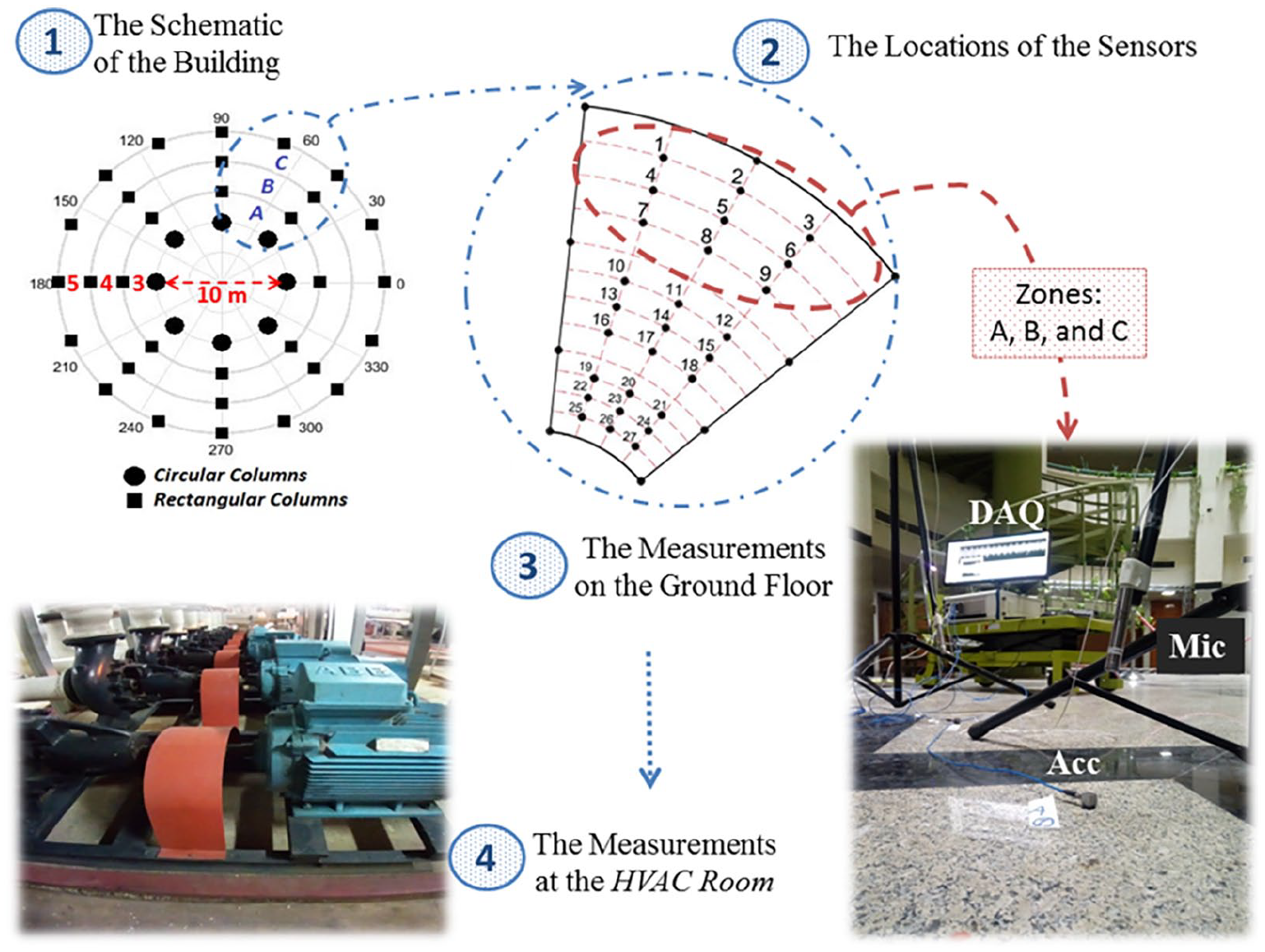
The measurement procedure.

With the objective of identifying the origin of the unfamiliar vibration, the initial phase of the measurement process was centered on the Heating, Ventilation, and Air Conditioning (HVAC) room and its constituent equipment components, (Figure 1). Through a comparative analysis of the data extracted from the HVAC room with the measurements collected from the ground floor, it becomes possible to diagnose the vibration’s source based on the operational frequencies.

System identification

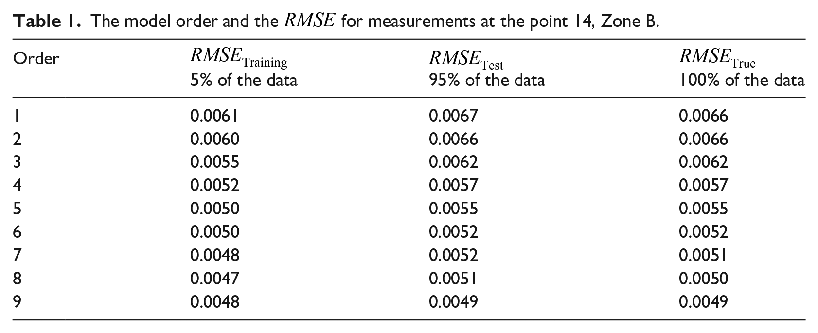
Table 1 presents a comparison of the ${RMSE}_{Training}$ , ${RMSE}_{Test}$ , and ${RMSE}_{True}$ results using different model orders. This is done to select the most suitable order that strikes a balance between ${RMSE}_{True}$ and computational cost. Despite the fact that Table 1 shows the lowest ${RMSE}_{True}$ value is associated with the ninth order, the seventh order is chosen for the fitting process to avoid excessive computational costs since the error changes were small.

Table 1.

The model order and the $R M S E$ for measurements at the point 14, Zone B.

Order	$R M S E_{Training}$ 5% of the data	$R M S E_{Test}$ 95% of the data	$R M S E_{True}$ 100% of the data
1	0.0061	0.0067	0.0066
2	0.0060	0.0066	0.0066
3	0.0055	0.0062	0.0062
4	0.0052	0.0057	0.0057
5	0.0050	0.0055	0.0055
6	0.0050	0.0052	0.0052
7	0.0048	0.0052	0.0051
8	0.0047	0.0051	0.0050
9	0.0048	0.0049	0.0049

Once the model has been determined, the next step is to apply the model to the data. The measurement process begins with the HVAC room, as it is believed to be the probable source of the unidentified vibration. This room is situated on the underground floor in zones B and C. Figure 2 displays the outcome of implementing the suggested method using the gathered data from the HVAC room. It should be highlighted that the histograms presented in the figure were created using an edge control approach to categorize the results within each frequency range with a resolution of 0.1 Hz.

Figure 2.

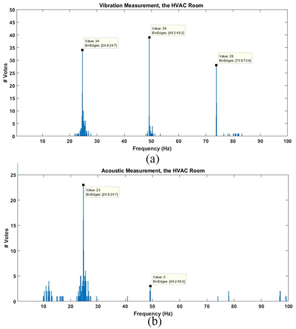
The results of the proposed method: (a) the results of the proposed method apply to the acoustic measurement data and (b) the results of the proposed method apply to the acoustic measurement data.

The proposed approach yields commensurate outcomes when both acoustic and vibration signals are employed, a facet that can be construed as advantageous. To corroborate the credibility of these findings, the Frequency Domain Decomposition (FDD) technique is enlisted. Comprehensive insights into the method, its intricacies, and its formulation are provided in the appendix for reference. This methodology serves to affirm the obtained results through an exposition of the Singular Values associated with the Power Spectral Density (PSD) matrix, extracted from the acoustic and vibration responses.

As explicitly portrayed in Figure 3, the graphical representation distinctly delineates that the predominant source of vibration is distinctly associated with the operational behavior of the water pumps situated within the cooling towers. More specifically, the ABB type 3GAA 182052 pumps, characterized by a rotational speed of 1480 RPM (equivalent to 24.66 Hz), emerge as the discernible cause behind this prominent vibrational pattern.

Figure 3.

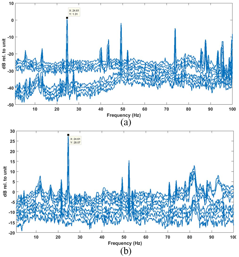
The validation results in the HVAC room: (a) the vibration response at the isolation pad of the ABB water pumps and (b) the acoustic response at the isolation pad of the ABB water pumps.

In the following important phase, we collected data concerning the vibration and acoustic responses occurring on the ground floor. To do this, we utilized accelerometers and microphones that were positioned within different areas identified as Zones A, B, and C. It’s notable that the microphones were positioned slightly above the floor surface, approximately 10 cm, and were placed at the same spots as the accelerometers.

Subsequently, we applied the recommended system identification method to scrutinize this collected data. The results stemming from the employed System Identification (SI) technique are visually presented in Figure 4. This depiction specifically highlights the measurements taken from Point 23 within Zone A, Point 14 within Zone B, and Point 5 within Zone C.

Figure 4.

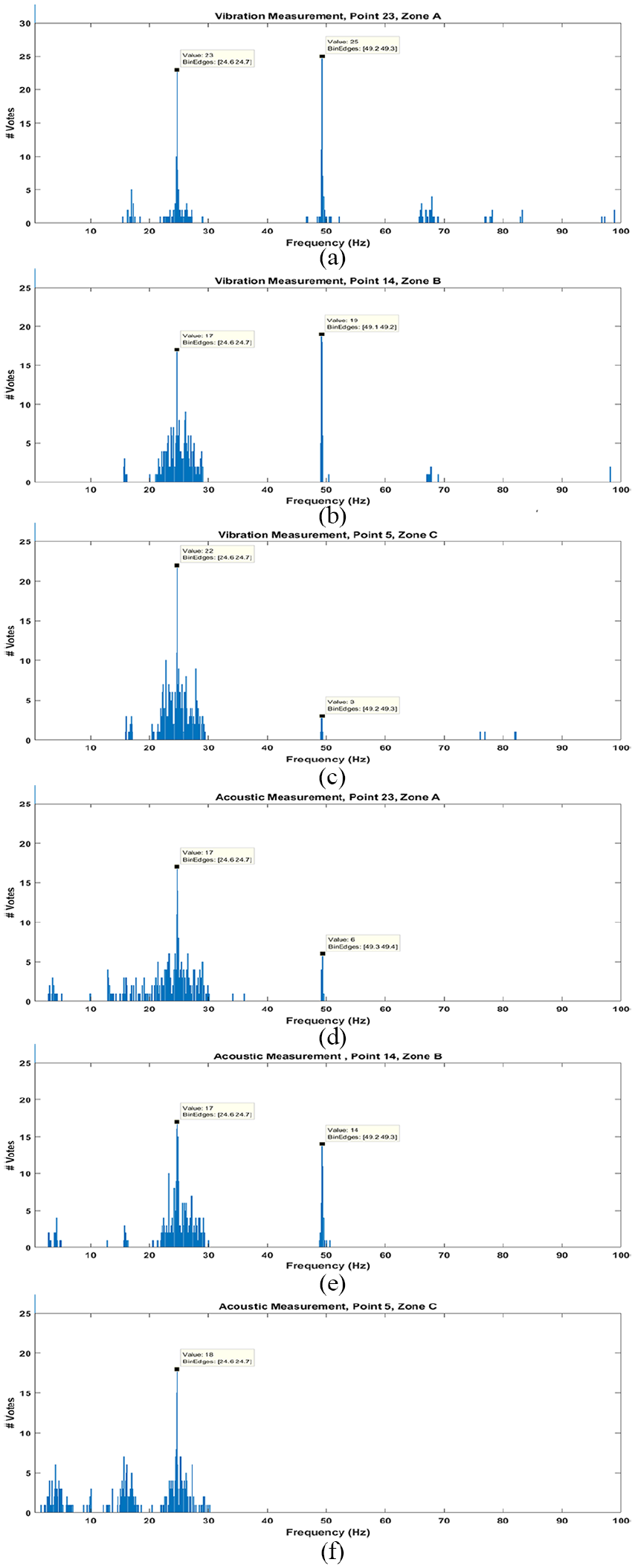
The results of the proposed System Identification (SI) method on the ground floor: (a) results using the Vibration Response, Point 23, Zone A, (b) results using the Vibration Response, Point 14, Zone B, (c) results using the Vibration Response, Point 5, Zone C, (d) results using the Acoustic Response, Point 23, Zone A, (e) results using the Acoustic Response, Point 14, Zone B, and (f) results using the Acoustic Response, Point 5, Zone C.

These diagrams clearly show the main frequency and its harmonics. This suggests that the peaks we see in the histograms might be connected to the functioning of rotating machinery and vibrations at harmonious intervals. Although there are some small differences in the results between the acoustic and vibration diagrams, it seems that the suggested SI method gives similar signs of identification when we use both acoustic and vibration measurements.

To double-check the correctness of these histograms, we used the FDD method on the measurements taken from the ground floor. Unlike the earlier method we described, where we only used one point in each zone (Point 23 in Zone A, Point 14 in Zone B, and Point 5 in Zone C), here we use all the measurements, including both acoustic and vibration responses, to confirm these findings. Figure 5 illustrates the process of figuring out things in the frequency domain. This is done by using a technique called singular value decomposition on a kind of matrix called the power spectral density matrix.

Figure 5.

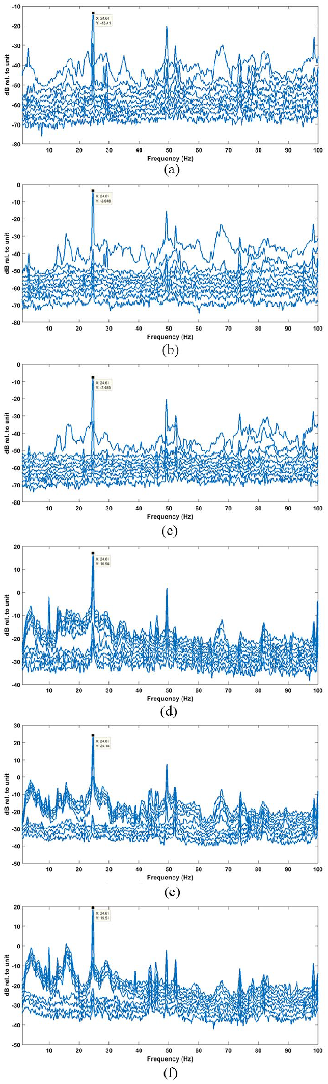
The validation results using the FDD method: (a) results using the Vibration Response, Zone A, (b) results using the Vibration Response, Zone B, (c) results using the Vibration Response, Zone C, (d) results using the Acoustic Response, Zone A, (e) results using the Acoustic Response, Zone B, and (f) results using the Acoustic Response, Zone C.

The figures show that the dominant frequency of the forced vibration (24.6 Hz) is evident in all diagrams within each zone. Thus, it seems plausible that the structure is the (indirect) source of the vibration issue.

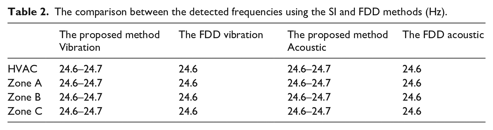
Table 2 summarizes the results of the proposed system identification method and the results of the implementation of the FDD method as a means of validation. The ability and accuracy of the proposed SI method to detect the exciting frequency of the unknown forced vibration are clearly proven.

Table 2.

The comparison between the detected frequencies using the SI and FDD methods (Hz).

	The proposed method Vibration	The FDD vibration	The proposed method Acoustic	The FDD acoustic
HVAC	24.6–24.7	24.6	24.6–24.7	24.6
Zone A	24.6–24.7	24.6	24.6–24.7	24.6
Zone B	24.6–24.7	24.6	24.6–24.7	24.6
Zone C	24.6–24.7	24.6	24.6–24.7	24.6

Response estimation (RE)

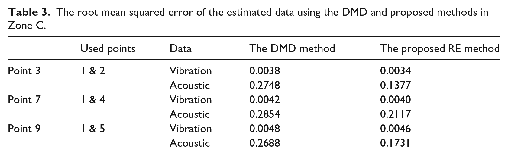
In this part, we’re looking to figure out how a new point will respond over time using the data we have from two other points. The condition is that all these points should be in the same area and set up in the same way. To help understand, let’s consider an example involving three estimates in zone C. This is to practically show how well the method we are proposing really works. To explain this more concretely: Imagine we want to know how point 3 will react, and we do this by using the data we already have from points 1 and 2. Then, we move on to point 7 and estimate its response using measurements from points 1 and 4. Lastly, we are interested in point 9, and we estimate its response by looking at the data from points 1 and 5. This helps us see how well our approach works in a real-world situation.

Table 3 illustrates the root mean squared error of the estimated data, which is calculated using the formula $\sum_{i = 1}^{N} \sqrt{\frac{{({\hat{X}}_{i} - X_{i})}^{2}}{N}}$ . The results demonstrate the ability to accurately track the primary frequencies, as depicted in Figures 6 and 7. However, it appears that the estimation method could benefit from a more sophisticated variable coefficient to achieve a higher level of accuracy when fitting the data.

Table 3.

The root mean squared error of the estimated data using the DMD and proposed methods in Zone C.

	Used points	Data	The DMD method	The proposed RE method
Point 3	1 & 2	Vibration	0.0038	0.0034
Point 3	1 & 2	Acoustic	0.2748	0.1377
Point 7	1 & 4	Vibration	0.0042	0.0040
Point 7	1 & 4	Acoustic	0.2854	0.2117
Point 9	1 & 5	Vibration	0.0048	0.0046
Point 9	1 & 5	Acoustic	0.2688	0.1731

Figure 6.

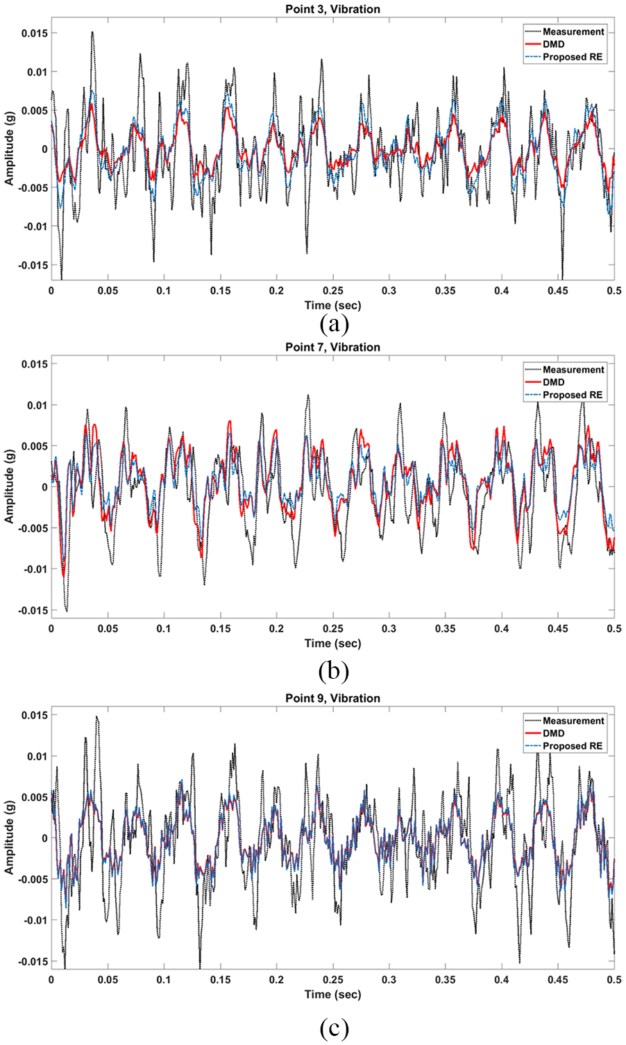
The results of the proposed response estimation method: (a) the proposed method applied to the vibration signals in Zone C, (b) the proposed method applied to the vibration signals in Zone C, and (c) the proposed method applied to the vibration signals in Zone C.

Figure 7.

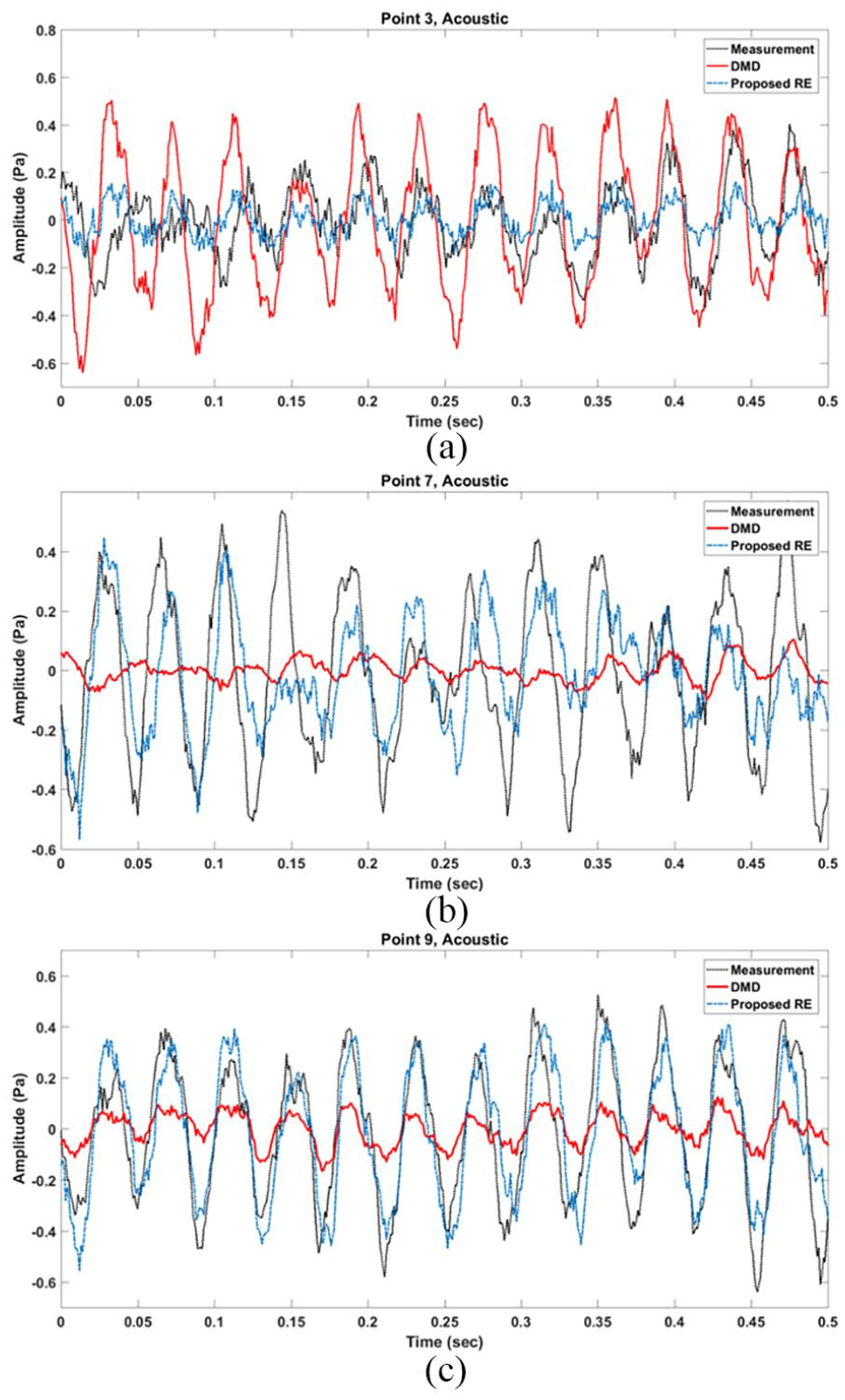
The proposed method applied to the acoustic signals in Zone C: (a) the proposed method applied to the acoustic signals in Zone C, (b) the proposed method applied to the acoustic signals in Zone C, and (c) the proposed method applied to the acoustic signals in Zone C.

Just like the process of estimating vibration responses, the Response Estimation (RE) method can also be used to predict the main pattern and frequencies using sound-based signals. However, it’s crucial to understand that the estimation procedure becomes more intricate when dealing with acoustic measurements. This complexity arises from a range of factors including ambient noises, intricate vibroacoustic challenges, as well as the interplay between airborne and structure-borne sounds.

In this study, we present data-driven techniques for both system identification and response estimation, employing a simplified framework of data-driven science. The utility of this method extends beyond its present application, rendering it adaptable to various other research domains such as Condition Monitoring (CM), vibration analysis, and industrial vibration tests. The demonstrated effectiveness and accuracy of our proposed approach indicate the potential for a fresh practical method in this field, albeit grounded in data from a single instance. For future studies, there is merit in trying to enhance this methodology through the incorporation of deep learning algorithms. These algorithms have exhibited superior efficacy in dealing with nonlinear and complex systems, suggesting their potential to further refine and amplify the capabilities of this approach.

Conclusion

Structural Health Monitoring (SHM) has stepped into a new phase thanks to data-driven techniques. In this research, we explored simplified data-driven methods for figuring out how systems work and predicting their responses. Our approach involves using a basic model that’s a bit like adding up different sine waves to match up with how things vibrate and make sounds over time. We use a histogram, which is like a chart, to turn this model into a way of understanding the different frequencies at different times. To make sure our findings are accurate, we also used a method called Frequency Domain Decomposition (FDD).

Additionally, we came up with a way to predict how things will respond over time, inspired by a technique known as Dynamic Mode Decomposition (DMD). We looked into an improved version of this DMD-based method to predict how things will respond in new places that are similar in shape. To show how well our method works, we used a real example of a concrete building that was having unexpected vibrations on its ground floor.

What we found is that our proposed System Identification (SI) method can spot unknown vibrations accurately, and our suggested Response Estimation (RE) method does a better job at predicting how vibrations and sounds change over time compared to the standard DMD method. The plus point of using our method is that it needs fewer measurements and sensors.

Looking ahead, we suggest focusing on using strong AI-based techniques to predict how things vibrate in more complex, nonlinear situations.

Footnotes

Appendix: Methodology of frequency domain decomposition (FDD)

This section provides a concise description of the key principles and formulation behind the Frequency Domain Decomposition (FDD) technique, as well as references to relevant sources.^15,16 The fundamental idea of this method lies in the representation of the Frequency Response Function (FRF) through partial fractions, involving poles and residues:

(A.1)

H (j ω) = \sum_{k = 1}^{n} \frac{R_{k}}{j ω - λ_{k}} + \frac{{\bar{R}}_{k}}{j ω - λ_{k}}

(A.2)

λ_{k} = - ξ_{k} ω_{dk} = - ξ_{k} ω_{k} + j ω_{k} {(1 - ξ_{k}^{2})}^{1 / 2}

(A.3)

R_{k} = ϕ_{k} γ_{k}

where $ϕ_{k}$ and $γ_{k}$ represent the mode shape and the modal participation vectors. Then, formula A.4 presents the relationship between the unknown inputs $x (t)$ and the measured responses $y (t)$ as,

(A.4)

G_{yy} (j ω) = \bar{H} (j ω) G_{xx} (j ω) H {(j ω)}^{T}

where $G_{xx} (j ω)$ is pertaining to the $(r \times r)$ power spectral density (PSD) matrix of the input, $r$ is the number of inputs, $G_{yy} (j ω)$ is the $(m \times m)$ PSD matrix of the responses, $m$ is the number of responses, $H (j ω)$ corresponds the $(m \times r)$ Frequency Response Function (FRF) matrix and finally the overbar and superscript $T$ denote the complex conjugate and transpose, respectively. By considering the input as a white noise, that is, its PSD is a constant matrix ( $G_{xx} (j ω) = C$ ), so equation (A.4) becomes

(A.5)

G_{yy} (j ω) = \sum_{k = 1}^{n} \sum_{s = 1}^{n} [\frac{R_{k}}{j ω - λ_{k}} + \frac{{\bar{R}}_{k}}{j ω - \bar{λ_{k}}}] C [\frac{R_{s}}{j ω - λ_{s}} + \frac{{\bar{R}}_{s}}{j ω - \bar{λ_{s}}}]

where superscript $H$ denotes a complex conjugate and transpose. Multiplying the two partial fraction factors and making use of the Heaviside partial fraction theorem, and after some mathematical manipulations, the output PSD can be presented as a pole/residue form, as expressed in formula A.6. The Matrix $A_{k}$ represents the kth residue matrix of the output PSD.

(A.6)

G_{yy} (j ω) = \sum_{k = 1}^{n} \frac{A_{k}}{j ω - λ_{k}} + \frac{{\bar{A}}_{k}}{j ω - - λ_{k}} + \frac{B_{k}}{- j ω - λ_{k}} + \frac{{\bar{B}}_{k}}{- j ω - - λ_{k}}

Declaration of conflicting interests

The author(s) declared no potential conflicts of interest with respect to the research, authorship, and/or publication of this article.

Funding

The author(s) received no financial support for the research, authorship, and/or publication of this article.

ORCID iD

Afshar Kasaei

References

Gordan

Sabbagh-Yazdi

Ismail

, et al. State-of-the-art review on advancements of data mining in structural health monitoring. Measurement 2022; 193: 110939.

Zhang

Mousavi

Masri

, et al. Vibration feature extraction using signal processing techniques for structural health monitoring: A review. Mech Syst Signal Process 2022; 177: 109175.

Liu

Bao

Machine learning-based stochastic subspace identification method for structural modal parameters. Eng Struct 2023; 274 : 115178.

Yang

Nagarajaiah

Blind modal identification of output-only structures in time-domain based on complexity pursuit. Earthq Eng Struct Dyn 2013; 42(13): 1885–1905.

Yao

, et al. Blind modal identification in frequency domain using independent component analysis for high damping structures with classical damping. Comput Aided Civ Infrastruct Eng 2018; 33(1): 35–50.

Bao

Chen

Wei

, et al. The state of the art of data science and engineering in structural health monitoring. Engineering 2019; 5(2): 234–242.

Ibrahim

SR.

A time domain vibration test technique, 1973.

Chen

, et al. Application of decoupled ARMA model to modal identification of linear time-varying system based on the ICA and assumption of ‘short-time linearly varying. J Sound Vib 2021; 499: 115997.

IIIJames

Carne

Lauffer

JP.

The natural excitation technique (NExT) for modal parameter extraction from operating wind turbines. Sandia National Labs., Albuquerque, NM (United States), 1993.

10.

Juang

J-N

Pappa

RS.

An eigensystem realization algorithm for modal parameter identification and model reduction. J Guid Control Dyn 1985; 8(5): 620–627.

11.

Caicedo

JM.

Practical guidelines for the natural excitation technique (NExT) and the eigensystem realization algorithm (ERA) for modal identification using ambient vibration. Exp Tech 2011; 35: 52–58.

12.

Van Overschee

De Moor

Subspace identification for linear systems: Theory—Implementation—Applications. Boston: Springer Science & Business Media, 2012.

13.

Peeters

De Roeck

Reference-based stochastic subspace identification for output-only modal analysis. Mech Syst Signal Process 1999; 13(6): 855–878.

14.

Fan

Hao

Improved automated operational modal identification of structures based on clustering. Struct Control Health Monit 2019; 26(12): e2450.

15.

Brincker

Zhang

Andersen

Modal identification from ambient responses using frequency domain decomposition. In: Presented at the Proceedings of the 18th international modal analysis conference (IMAC), San Antonio, TX, USA, 2000, pp.625–630.

16.

Brincker

Zhang

Andersen

Modal identification of output-only systems using frequency domain decomposition. Smart Mater Struct 2001; 10(3): 441–445.

17.

Isavand

Peplow

Kasaei

Performing building vibration assessments by acoustic measurements. Build Acoust 2020; 27(1): 21–33.

18.

Huang

Shen

Long

, et al. The empirical mode decomposition and the Hilbert spectrum for nonlinear and non-stationary time series analysis. Proc R Soc Lond A Math Phys Sci 1998; 454(1971): 903–995.

19.

Antoni

Blind separation of vibration components: Principles and demonstrations. Mech Syst Signal Process 2005; 19(6): 1166–1180.

20.

Hyvärinen

Oja

Independent component analysis: algorithms and applications. Neural Netw 2000; 13(4-5): 411–430.

21.

Karhunen

Oja

Wang

, et al. A class of neural networks for independent component analysis. IEEE Trans Neural Netw 1997; 8(3): 486–504.

22.

Kerschen

Poncelet

Golinval

J-C.

Physical interpretation of independent component analysis in structural dynamics. Mech Syst Signal Process 2007; 21(4): 1561–1575.

23.

Amini

Hedayati

Underdetermined blind modal identification of structures by earthquake and ambient vibration measurements via sparse component analysis. J Sound Vib 2016; 366: 117–132.

24.

Brownjohn

JMW

Hester

Enhanced sparse component analysis for operational modal identification of real-life bridge structures. Mech Syst Signal Process 2019; 116: 585–605.

25.

Yang

Nagarajaiah

Output-only modal identification with limited sensors using sparse component analysis. J Sound Vib 2013; 332(19): 4741–4765.

26.

Yang

Bai

Estimation of modal parameters using the sparse component analysis based underdetermined blind source separation. Mech Syst Signal Process 2014; 45(2): 302–316.

27.

Zhou

Chen

, et al. Output-only modal estimation using sparse component analysis and density-based clustering algorithm. Measurement 2018; 126: 120–133.

28.

Wei

Jin

General solutions for nonlinear differential equations: a rule-based self-learning approach using deep reinforcement learning. Comput Mech 2019; 64: 1361–1374.

29.

Han

Jentzen

. Solving high-dimensional partial differential equations using deep learning. Proc Natl Acad Sci 2018; 115(34): 8505–8510.

30.

Leng

Gardoni

Wang

, et al. Condition-based structural health monitoring of offshore wind jacket structures: Opportunities, challenges, and perspectives. Struct Health Monit 2023; 22(5): 3558–3575.

31.

Yan

Yuen

K-V

, et al. An adaptive variational mode extraction method based on multi-domain and multi-objective optimization for bearing fault diagnosis. Struct Health Monit 2023; 22(4): 2708–2733.

32.

Kong

Qin

Wang

, et al. Data-driven dictionary design–based sparse classification method for intelligent fault diagnosis of planet bearings. Struct Health Monit 2022; 21(4): 1313–1328.

33.

Ding

Huang

Shen

, et al. Synchroextracting frequency synchronous chirplet transform for fault diagnosis of rotating machinery under varying speed conditions. Struct Health Monit 2023; 0(0): 14759217231181308 DOI: 10.1177/14759217231181308

34.

Guo

Yang

, et al. A local modulation signal bispectrum for multiple amplitude and frequency modulation demodulation in gearbox fault diagnosis. Struct Health Monit 2023; 22(5): 3189–3205.

35.

Laura

PAA

Duran

. A note on forced vibrations of a clamped rectangular plate. J Sound Vib 1975; 42(1): 129–135.

36.

Brunton

Kutz

JN.

Data-driven science and engineering: Machine learning, dynamical systems, and control. Cambridge: Cambridge University Press, 2019.

Enhancing response estimation and system identification in structural health monitoring through data-driven approaches

Abstract

Keywords

Introduction

Theory

Methodology

System identification (SI)

Response estimation (RE)

Results and discussion

Test setup

System identification

Response estimation (RE)

Conclusion

Footnotes

Appendix: Methodology of frequency domain decomposition (FDD)

Declaration of conflicting interests

Funding

ORCID iD

References