A model study of low-frequency noise exposure indoors due to road traffic

Abstract

Indoor low-frequency noise levels due to road traffic has been modelled for facade examples consisting of a lightweight steel facade, a concrete facade and two types of windows. Possible audibility of heavy vehicles passing by has been investigated as well as the dependence of the exposure level on driving speed and distance to road. The results show that pass-by events may be audible at low frequencies for cases complying with building standards and noise guideline values exemplified by Swedish regulation. Moreover, the A-weighted levels may be dominated by low frequency noise, and the frequency of occurrence of pass-by traffic noise events may be sufficiently high to create disturbance for typical traffic situations. Furthermore, it is shown that the contribution of pass-by events to the equivalent level indoors may increase when the driving speed is lowered.

Introduction

Many urban central locations are attractive to builders of new homes, but the residents may become disturbed by the traffic noise from the street. Annoyance and sleep disturbance due to road traffic noise in urban areas have been estimated to constitute the major part of the total disease burden due to environmental noise in western Europe. ¹ Within the EU, the public health issue of environmental noise is addressed via harmonised noise mapping with publicly available results as well as action planning on short and long term. ² The indicators of the noise mapping are based on A-weighted long-term averages: the day-evening-night level, L_den, and the night level, L_n. ² Depending on the urban situation, the road traffic noise may be dominated by contributions from the nearest road or from traffic in a larger area. Especially for facade positions on closed inner yards or on high-rise buildings, it has been shown that traffic sources within a larger urban area effectively contributes to the noise exposure levels (e.g. Ögren and Forssén, ³ Ögren and Kropp, ⁴ Meyerson, ⁵ and Benocci et al. ⁶ ). The present paper, however, focuses on cases of the former situation, that is, with dwellings that have a local road nearby.

When urban areas are densified and housing is built closer to a busy street, the acoustic dimensioning of the facade is stepped up to meet the indoor sound requirements. These facade constructions above all provide improved sound insulation at medium and high frequencies, while the sounds at low frequencies do not become as much quieter. A significant reduction at low frequencies, for example, at around 50 Hz and below, will be technically far-reaching and costly, so it would probably not be fulfilled without supplemented legislation. We might therefore expect a more low-frequency character of the traffic noise indoors when we build closer to streets or at other noisy locations in urban densification projects.

Another effect is that the number of audible passages may be significantly increased if housing is built closer to roads, even though the facade sound insulation is stepped up to meet the existing requirements. Whereas the commonly used equivalent noise level indicators, like L_den, L_night and L_Aeq24h, capture an energy average over multiple hours, the audibility of a passage is rather linked with its peak or maximum value, for example, described by the indicator L_AFmax. Audibility of noise events, for example, in terms of number of events or intermittency, has recently gained an increased interest within environmental noise research (e.g. Wunderli et al. ⁷ and Brink et al. ⁸ ). When decreasing the distance to a road, the rate of increase of the equivalent noise level with distance is smaller than that of the peak level. As a result, as we build closer to the roads, many of the peaks in sound level, for example, when buses and trucks pass by, may become audible when they end up both above our hearing threshold and above the equivalent level indoors (e.g. contributed by installation noise) thereby not being masked. For both of these aspects, that is, low-frequency noise and audible events, the applicable regulation on indoor sound environment may still be met.

Since road traffic noise in urban areas already dominates the estimated disease burden due to environmental noise in Europe, at the same time as activities of urban densification are widespread, the resulting issues of possible increase in indoor low-frequency noise and audible events are deemed relevant.

The most commonly used indicators, that is, L_den, L_night and L_Aeq24h (as well as L_AFmax) use A-weighting. In addition, most regulations have a limited frequency range; instead of including frequencies from for example, 20 or 25 Hz, a range starting from 50 or 125 Hz is common. Thereby, the fulfilment of an indoor limit value measured as L_den, L_night or L_Aeq24h is relatively insensitive to low-frequency noise. Many countries use additional guidelines for indoor noise at low frequencies, formulated as equivalent levels in one-third octave bands, as for example, in the Swedish guidelines for indoor noise where the one-third octave bands from 31.5 to 200 Hz are covered. ⁹ Concerning the peak levels, some countries (e.g. among the Nordic countries) apply limits also on the maximum level, for example, indicator L_AFmax, with a usual limit value being 15 dB higher than on the equivalent level, whereas most countries restrict their regulations to equivalent noise levels. In both cases the vehicle pass-by events may be audible, still fulfilling local regulation. Hence, we can identify the risk of significant disturbance due to a large number of audible traffic noise events with low-frequency (booming) character in newly built homes alongside busy roads. Previous research has shown that even with as few audible events as 2–8 per hour, the disturbance can increase markedly compared with a more even noise level. ¹⁰

The present paper contains results on two main parts: (1) possible low-frequency audibility of individual pass-by events and (2) expected variation in exposure level due to changes in driving speed and distance to road. In the first part it is shown that there are possibilities for a heavy road vehicle pass-by to be audible indoors. This is made using a set of facade cases for a situation with a relatively short distance to road and using standardised hearing thresholds ¹¹ as well as Swedish regulations as an example to see what low-frequency audibility is possible at the same time as local legislation is fulfilled. For the second part, a parametric study is made where the distance to road as well as the vehicle speed is varied, enabling conclusions on the possible contributions of the pass-bys to the equivalent level in terms of their sound exposure levels.

To reach these results, and their conclusion, the method section below contains the following parts: modelling of the outdoor noise exposure due to road traffic, modelling of peak and equivalent levels, a general description of acoustic performance of housing facades, prediction of indoor noise level due to outdoor exposure at facade, and a description of the facade examples used here, consisting of two facade types (light and heavy) and two window types (ordinary and soundproof).

Method

Modelling of noise exposure due to road traffic

To calculate the noise levels from road traffic, a separation of vehicle categories is made, for example, light vehicles, medium heavy vehicles, heavy vehicles and two-wheelers. The example case study made here follows Swedish regulations, which currently uses the two vehicle categories light and heavy vehicles (i.e. passenger cars and buses/trucks), of which here the focus is on the heavy vehicles. Road vehicles in general can be seen to have two main sound sources: due to the tyre-road contact and the engine (e.g. Forssén et al. ¹² ). The tyre-road noise, also called rolling noise, is generated at the contact between the tyre and the road surface and usually dominates at higher driving speeds. Engine noise, also called propulsion noise (containing components of noise from engine, exhaust system, air intake, transmission, compressors, etc.), usually dominates at lower driving speeds. (The speed above which the rolling noise on average dominates over the propulsion noise is circa 30 km/h for light vehicles and circa 80 km/h for heavy vehicles. ¹³ )

The variation of the source strength with frequency and with driving speed for the road vehicles has here been calculated using a model from an EU project called Imagine. ¹³ This model uses a one-third octave frequency resolution, that is, the same resolution as commonly used for measuring and describing the reduction index of facade elements (e.g. International Organization for Standardization ¹⁴ ). The model is as well available in commercial software for noise mapping. It is also related to the model that is now entering into use for noise mapping within the EU (Cnossos-EU), ¹⁵ but the latter has a less fine frequency resolution (octave bands), whereby it is not used here. An alternative option could have been to use the Nordic-developed model Nord2000, but we chose here to use the Imagine model due to its close relation with the Cnossos-EU model (i.e. equal values in terms of octave bands) that is likely to be of future general use.

However, the current Swedish regulations use an older model (‘Nordic calculation model’ from 1996 ¹⁶ ) for the total, single number, A-weighted source strength as function of driving speed, v (km/h). The exposure level for a heavy vehicle at 10 m distance is there given by

$$L_{\mathrm{AE}}=80.5+30{\log }_{10}(v/50)(dB)$$

(1)

for driving speeds v ≥ 50 km/h (and L_AE = 80.5 dB for driving speeds between 30 and 50 km/h), whereas the corresponding model for the maximum level is

$$L_{\mathrm{AFmax}}=75+30{\log }_{10}(v/50)(dB)$$

(2)

for driving speeds ≥50 km/h (and L_AFmax = 75 dB for driving speeds between 30 and 50 km/h). The latter model, for the maximum level, is here used to define the total A-weighted level in calculation examples following Swedish regulation, given a spectral shape following the Imagine model. For the parametric study, later in the paper, only the Imagine source model is used.

In addition, individual vehicles are differently noisy. One can, for example, hear occasional noisy cars even if the ‘average car’ passes by inaudibly. This individual variation can be described with the help of a probability distribution of the strength, with parameters determined by vehicle type and driving speed. (In the Nordic calculation model from 1996, this is described for the two categories of light and heavy vehicles). Equation (2) defines the mean value of the maximum level.

The spectra of the source strengths, in terms of power levels L_W,roll for rolling noise and L_W,prop for propulsion noise, are modelled as follows. ¹³

$$L_{\mathrm{W},\mathrm{roll}}=a_{\mathrm{roll}}+b_{\mathrm{roll}}\cdot {\log }_{10}\left(\frac{v}{v_{\mathrm{ref}}}\right)$$

(3)

$$L_{\mathrm{W},\mathrm{prop}}=a_{\mathrm{prop}}+b_{\mathrm{prop}}\cdot \frac{v-v_{\mathrm{ref}}}{v_{\mathrm{ref}}}.$$

(4)

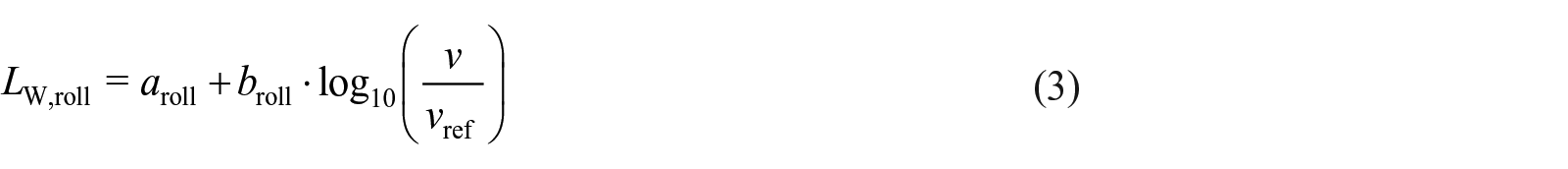
Here, v_ref = 70 km/h is the reference speed. The a and b coefficients are frequency dependent, as plotted in Figure 1. It can be noted that the speed dependence is logarithmic for L_W,prop and linear for L_W,prop, which captures the larger increase with driving speed of the rolling noise compared with the propulsion noise for low and medium-high driving speeds. The total power level, L_W, is the sum from energetic addition of the two components:

$$L_{\mathrm{W}}=10{\log }_{10}\left({10}^{L_{W,\mathrm{roll}}/10}+{10}^{L_{W,\mathrm{prop}}/10}\right).$$

(5)

Figure 1.

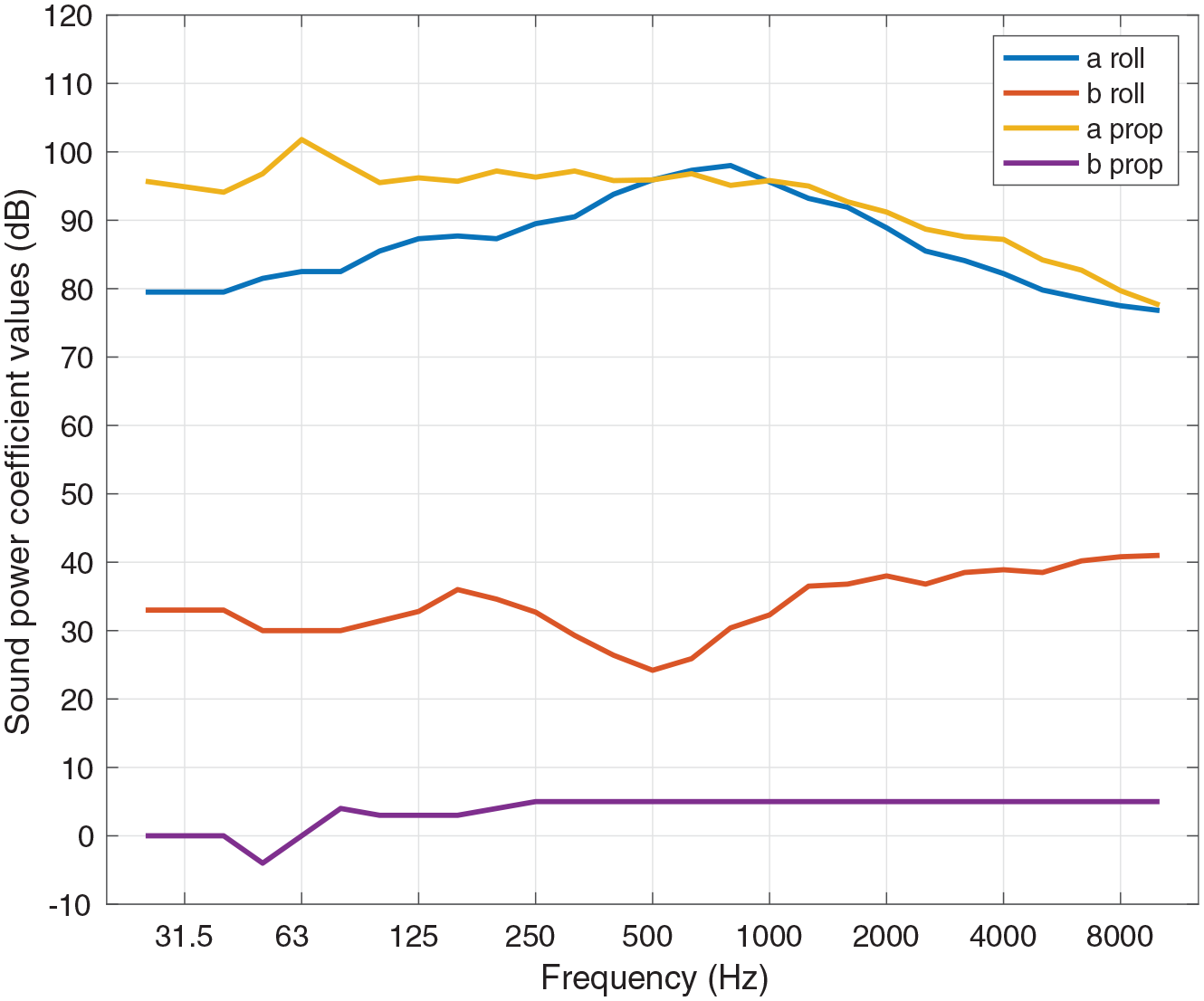
Sound power level coefficients for heavy vehicles.

In Figure 2 the output power level, LW, of a heavy vehicle is plotted as function of frequency for various driving speeds, both as unweighted and A-weighted levels. The peak at around 63 Hz, most prominent for the unweighted levels, is related to the engine speed. It can also be seen (in both plots), that the variation of LW with driving speed is small for frequencies below 80 Hz, which links with the b-coefficients shown in Figure 1.

Figure 2.

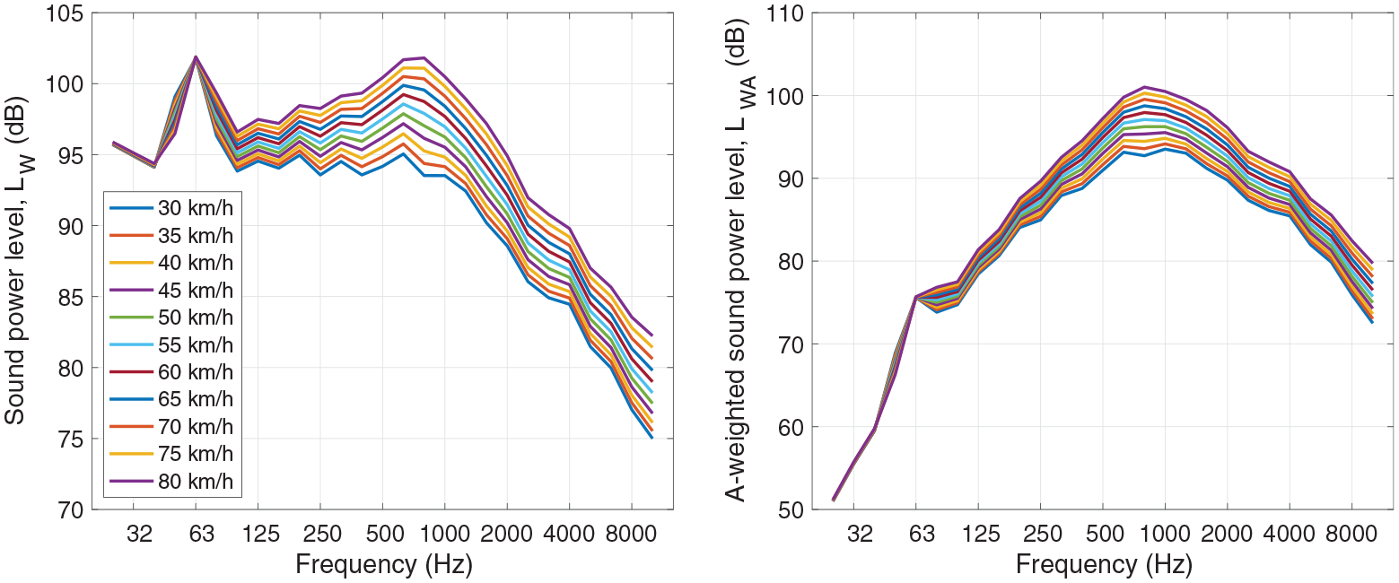
Sound power level of a heavy vehicle plotted as function of frequency for driving speeds ranging from 30 to 80 km/h. Unweighted L_W (left) and A-weighted L_WA (right).

Peak and equivalent levels

To estimate the peak and equivalent levels of road traffic, as a starting point each road vehicle is seen as an omnidirectional source with constant acoustic power, which moves along a straight line with a constant speed, U (m/s), much lower than the speed of sound. (See geometry in Figure 3) For a single road vehicle located at position x along the road, the instantaneous sound pressure level, L_p (dB), can be written

$$L_{\mathrm{p}}=L_{\mathrm{W}}-10{\log }_{10}\left(4\pi r^2\right)+\Delta L_{\mathrm{EA},\mathrm{P2P}}$$

(6)

where L_W (dB) is the power level of the source and r is the horizontal distance between source and receiver such that r² = L² + x², where L is the shortest horizontal distance between road and receiver. The part L_p = L_W − 10log₁₀(4πr²) derives from spherical spreading from a point source and the correction ∆L_EA,P2P is the excess attenuation due to point-to-point propagation above a ground surface from the source location to the receiver location. Here, it is assumed that ∆L_EA,P2P is a constant with a value of 6 dB (i.e. an amplification as from pressure doubling) modelling propagation above hard ground with the source located close to the ground surface. (For the cases studied here, the discrepancy between a full calculation of interference pattern for hard ground and the 6 dB approximation was calculated to not be larger than 0.1 dB, assuming a source height according to the Cnossos-EU model of 0.05 m.)

Figure 3.

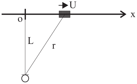
Geometry of the pass-by situation. The vehicle moves at constant speed U (m/s) along a straight line in the positive x-direction. The shortest distance, L, between the road (i.e. the U-axis) and the receiver is marked as a line that cuts the U-axis at U = 0. At time t, the vehicle is positioned at x = Ut and its distance to the receiver is $r=\sqrt{L^2+x^2}$ .

Assuming also constant driving speed such that L_W is constant, the highest level is attained at point of passage, that is, for x = 0, where r = L, for which the sound pressure level becomes

$$L_{\mathrm{PEAK}}=L_{\mathrm{W}}-10{\log }_{10}\left(4\pi L^2\right)+6.$$

(7)

By performing an energy average for an infinitely long line of source positions, the resulting equivalent level for a single vehicle can be written

$$L_{\mathrm{Eq}}=L_{\mathrm{W}}-10{\log }_{10}\left(4LUT\right)+6$$

(8)

where U is the driving speed in m/s and T is the integration time for the equivalent level. The corresponding exposure level is

$$L_{\mathrm{E}}=L_{\mathrm{W}}-10{\log }_{10}\left(4LU\right)+6$$

(9)

given by confining all energy to a 1-s interval, that is, equal to setting x = 1 (s) in equation (8). A derivation of equations (8) and (9) can be found in Appendix A.

Whereas equation (8) is for a single vehicle, the corresponding result for N vehicles per second can be found from energy addition, that is, based on the assumption that the contributions from different vehicles are uncorrelated, resulting in

$$L_{\mathrm{Eq}}=L_{\mathrm{W}}-10{\log }_{10}\left(4LU\right)+10{\log }_{10}\left(N\right)+6.$$

(10)

Using equations (7) and (10), the difference between the peak level, L_PEAK, and the equivalent level, L_Eq, can be written

$$L_{\mathrm{PEAK}}-L_{\mathrm{Eq}}=-10{\log }_{10}\left(\frac{\pi LN}{U}\right).$$

(11)

From equations (7), (10) and (11) it can be seen that the peak and equivalent levels have a difference in the distance decay, amounting to 10log₁₀(L); the 10log₁₀(4πL²) term of the peak level corresponds to a 6 dB decay per distance doubling whereas the 10log₁₀(4LU) term of the equivalent level corresponds to a 3 dB decay per distance doubling. (This is sometimes referred to as point source and line source behaviour, respectively.) It could be noted that the dependence of the equivalent level on the vehicle speed U, as seen in equation (10), might look counterintuitive, that is, that the equivalent level decreases with increasing vehicle speed. It can be seen as being due to the shorter time during which the vehicle is close to the receiver, the faster it moves. For the total, A-weighted level for an outdoor receiver, this effect is usually more than counterbalanced by the increase in power level with driving speed, but not necessarily so for a receiver indoors. This topic will be revisited in the Results section.

It should be noted that the above described modelling approach is restricted to simplified situations with hard and flat ground as well as neutral or slightly downward refracting atmosphere with also negligible influence of turbulence and air attenuation. These assumptions can be concluded to be reasonable for the situations studied here, with focus on low-frequency noise and a maximum distance to road of 100 m. Furthermore, it could be noted that the above described source modelling can have additional terms describing source directivity (e.g. Nota et al. ¹⁷ ). Such terms are however removed in the Cnossos-EU model ¹⁵ and are also omitted here for simplicity. Further existing source term corrections, not included here, involve road surface type, road surface temperature, tyre type, acceleration and road slope. ¹⁵

Acoustic performance of housing facades

Through windows, ventilation and the remaining facade towards the road, the traffic sounds are transmitted into the dwelling. Most of the sound usually passes through the windows, but at low frequencies the contribution through the facade material can be significant. For new buildings, the contribution of traffic sounds via adequate ventilation equipment to the indoor level can be assumed to be negligible.

According to the fundamental mass-law behaviour, the transmitted energy decreases with the square of the mass of the material (mass per unit area) and with the square of the frequency. That the transmission decreases with frequency means that the sound indoors gets a more low-frequency character than the sound outdoors, in addition to the whole level being reduced. While the mass-law largely determines the amount of transmission and overall frequency dependence of the facade elements, individual resonances and resonance phenomena can have a significant impact.

Windows and facade walls constructed as multilayer constructions with intermediate air gaps provide double-wall resonances with increased transmission at single, relatively narrow frequency ranges, typically at 50 Hz or lower for acoustically demanding, ‘soundproof’, constructions. At the same time, multilayer constructions provide a significantly increased sound insulation at higher frequencies, without having to use extra mass. For example, a two-layer construction provides, in comparison with the mass-law behaviour, an increased sound insulation in the entire frequency range above the region of the double-wall resonance.

For heavier facade constructions, for example, of concrete, the coincidence phenomenon may lower the sound insulation within a limited frequency range, typically at around 50–100 Hz. This is due to the coupling between the sound field and the bending motion of the building element; the dip in sound insulation appears in the vicinity of the critical frequency, where the frequency-dependent bending wave speed equals the sound speed in air. For frequencies above the coincidence dip, the sound insulation is usually above that of the mass-law behaviour. The mass-law is derived assuming a single-leaf panel without bending stiffness. It is therefore valid for single-leaf elements below the critical frequency and for double-left elements below the double-wall resonance frequency. Except for reduction index dips in the vicinity of these frequencies, the sound insulation can be expected to not be lower than what the mass-law predicts. And, below these frequencies, the sound insulation cannot be expected to be better than what the mass-law predict. For further reading on sound insulation by building elements, see for example, Vigran ¹⁸

The sound insulation also depends on the room’s size, acoustic absorption and resonance frequencies, especially at low frequencies. The room absorption is usually described by the reverberation time of the room (with an assumed value of 0.5 s regardless of frequency, according to Swedish regulations). By low-frequency we here mean 20–200 Hz, but in some cases even lower frequencies can be audible.

Prediction of indoor noise level

The indoor noise level, L_indoor, is calculated using a standardised procedure based on an approximate model, which can be formulated as follows. ¹⁴

$$L_{\mathrm{indoor}}=L_{2\mathrm{m}}-R+10{\log }_{10}\left(\frac{S}{A}\right).$$

(12)

Here, L_2m (dB) is the outdoor noise level 2 m in front of the facade (the free field level plus 3 dB), R is the acoustic reduction index of the facade element, S is the area of the facade element and A is the room’s absorption area equal to A = 0.16V / T₆₀, where V is the room volume and T₆₀ the reverberation time, here assumed to be 0.5 s. L_indoor can be calculated separately for the different facade elements (i.e. here window and remaining facade) and added energetically to provide the final indoor level. This approach assumes diffuse field, which means that the resulting indoor level is representative to positions not close to room boundaries, and that the uncertainty increases at lower frequencies due to room resonances.

When a new facade element (window, ventilation device or facade construction) is developed for the market, a laboratory measurement of its reduction index is made according to a standardised method assuming diffuse field. With these data, one can, for each frequency, calculate the total reduction index for a planned facade with its constituent sub-elements. The outdoor–indoor level difference, D (in dB), is defined as D = L_2m − L_indoor.

Facade examples

A modern lightweight facade with a steel frame and a modern heavy sandwich facade of concrete have been used in the calculation examples, both with generally good sound insulation ability. Two different modern windows have been used. One is a triple-glazed, ‘soundproof’, window specially adapted for high noise reduction and the other is a more common window, however double-glazed and can be considered to be of good acoustic quality. The corresponding reduction indices are based on measured windows and facade constructions, displayed in Figure 4. (Detailed data are provided in a freely available report. ¹⁹ ) Furthermore, we have assumed that the length of the facade is 3 m, the height is 2.5 m and the depth of the room is 4 m, thus modelling a typical bedroom with 12 m2 floor area. (We have not included noise via ventilation devices since only the worst solutions give a measurable impact and these solutions are generally avoided for new buildings in noisy environments.)

Figure 4.

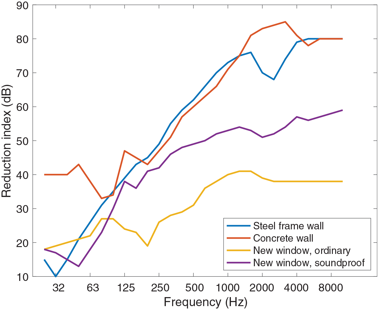
Reduction index of the four facade elements used: two walls and two windows.

Figure 5 shows the outdoor–indoor level difference, D (in dB), as resulting from the four combinations of the two wall constructions (steel frame and concrete) and the two types of window with an area of 1 m² (as is used for the second part of the results). It can be seen in Figure 5 that the performance at the lowest frequencies is linked with the wall type, where the lightweight (steel frame) facade performs worse than the heavyweight (concrete) facade. On the other hand, at higher frequencies (above circa 100 Hz), the window type is seen to determine the behaviour, that is, the soundproof window provides a better sound insulation than the ordinary window. Furthermore, the double-wall resonance of the soundproof window, at around 50 Hz, causes a dip in the sound reduction which is seen to impair the otherwise good performance of the heavyweight facade with soundproof window. The resulting indoor level is plotted in Figure 6 for a situation with the road at L =10 m distance from the facade and for a vehicle driving at 30 km/h. The results in Figure 6 also show that the low-frequency components of heavy road vehicles may dominate the total A-weighed level indoors, here apparent at 50 and 63 Hz for the facade cases with soundproof window.

Figure 5.

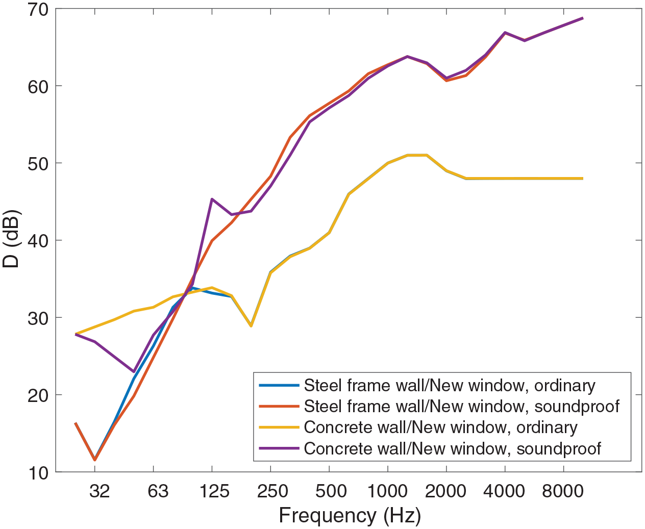
Sound pressure level difference, D = L_outdoors,2m − L_indoors (dB), for the four used facades, from combining the two wall types and the two window types.

Figure 6.

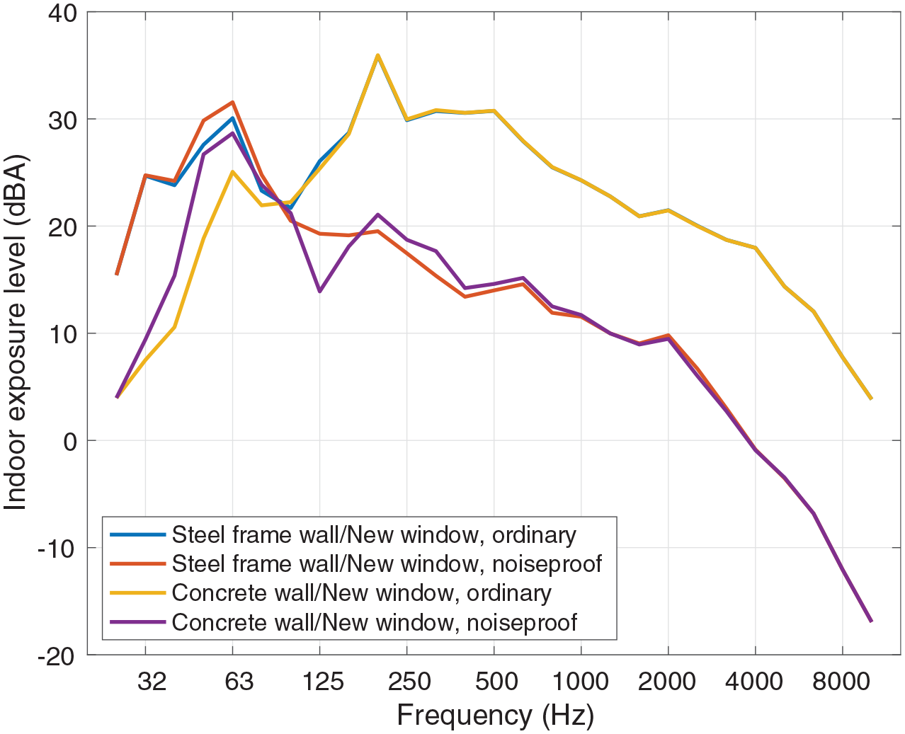
A-weighted indoor exposure level in dB for the four used facades, for a driving speed of 30 km/h and 10 m distance to road.

Results

The calculated examples shown here assume hard, flat ground, a straight road and vehicles passing by at constant speed. Also, open terrain is assumed on the opposite side of the road from the house. (In densified areas there is usually an additional urban canyon effect, that is, due to buildings on both sides of the street, which causes an amplification of the road traffic sound; however, this is omitted here for simplicity.)

Possible audibility of individual pass-by events

Figure 7 shows the unweighted spectrum of L_AFmax for a heavy vehicle passing by at a speed of 40 km/h at a distance of 12 m, for the example facade elements as described above, with a window area of 2 m. Comparing the noise level outdoors with the indoor levels for the different facades, one can see that the difference, and thus the sound insulation, tends to increase with frequency. (This trend becomes even clearer if also the mid-frequency range is included in the plot.) The peak in the outdoor level at about 60 Hz is due to engine noise and at that frequency the sound insulation of the facade is still relatively low. One therefore gets a typical frequency range around 60 Hz (here around 50–60 Hz) where the noise level inside may exceed both the hearing threshold curve and the Swedish Public Health Agency’s guideline values for low-frequency equivalent noise indoors.

Figure 7.

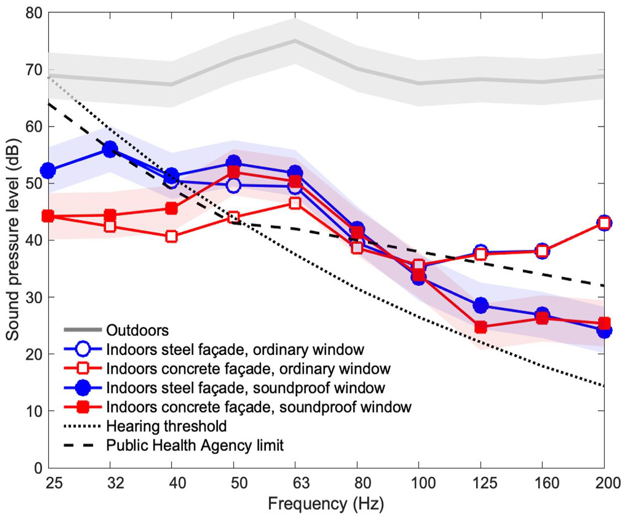
Sound pressure levels (with time-weighting FAST, i.e. as for calculating L_AFmax for a heavy vehicle (bus or truck), at 40 km/h, passing at a distance of 12 m. Plotted are: the outdoor level, indoor levels with light facade construction (‘steel facade’), with two different window types; the indoor level with heavy facade construction (‘concrete facade’), with two different window types; the hearing threshold curve (according to ISO 226 ¹¹ ); and the Swedish Public Health Agency limit values for low-frequency indoor noise (with an added data point at 25 Hz following Finnish regulations). The shaded areas at the curves represent the variation of individual vehicles (± one standard deviation according to the Nordic calculation model from 1996), exemplified for the outdoor level and for the two indoor level curves for the soundproof window.

This part of the sound can be assumed to have a large possibility to be audible. The fact that the sound at the maximum of the pass-by has a strength that is above the hearing threshold level means that a normal-hearing person on average can perceive it, in the absence of other, masking sounds. The fact that the noise levels at the maximum of the pass-by exceeds the low-frequency one-third octave band guideline values means that masking due to noise generated indoors, for example, from ventilation and fridge/freezer, is not likely to occur since such installation noise is forced to not exceed the same guideline values. These guideline values on the equivalent-level apply also to noise from outdoor sources in general whereby such noise will also not likely mask the peaks of the pass-by sounds. On the other hand, at about 100 Hz the sound from the passage is above the hearing threshold and might thus be audible, but it falls below the Public Health Agency’s curve and can thereby in many cases be masked by a steady background noise indoors, for example, from ventilation. Note that exceeding the Public Health Agency’s one-third octave band values is still allowed for individual vehicle pass-bys as long as the equivalent level, that is, time-averaged energy, is not exceeded. That the pass-by sounds have a large possibility to be audible is further substantiated by the coherence with recent work where detection of events assumes that they are 3 dB above the equivalent level.^7,20

The two curves that at 160 and 200 Hz show an indoor maximum level clearly above the Public Health Agency’s curve are calculated for a normal window, with ordinary but not poor sound insulation. This window can thus provide audible passages even at the upper part of the low-frequency range. The other two indoor noise level curves are for a special, ‘soundproof’ window where a very good sound insulation has been strived for.

An important factor for the degree of disturbance is the occurrence of audible passages (e.g. Brink et al. ⁸ , Waye et al. ¹⁰ ). Audibility depends partly on the traffic itself and on its proportion of heavy vehicles, but there are certain situations that are often problematic, for example, for road slopes when the engine load of heavy vehicles can increase, near bus stops where the buses accelerate and in urban canyons (with houses on both sides of a street), where a large gain at low frequencies can occur.

For a realistic traffic case example with 13,000 vehicles per day whereof 10% are heavy vehicles, one would get an average of about 80 heavy vehicles per hour during the day and about 20 per hour at night, for a typical daily distribution. (The daily distribution of heavy vehicles is taken from Kragh et al. ²¹ which suggests a default night-time proportion of 15% for urban or residential roads.) Most of these pass-bys can be assumed to be audible for the traffic situation exemplified here.

The estimated outdoor equivalent level is 65 dB (L_Aeq24h, free field level) in this case, which meets today’s Swedish noise requirements for smaller apartments, up to 35 m². Indoors, the corresponding equivalent level from the road traffic is estimated to be 20–28 dB for the various facades. Thereby the Swedish guideline value of 30 dB for the equivalent level indoors is also fulfilled.

The estimated maximum indoor level is 36–45 dB for the various facades. This is calculated, based on the variation of individual vehicles, as the maximum level (L_AFmax) which is only exceeded five times per average night, following Swedish regulation. (See e.g. Ref. ¹⁶ for a description of calculation.) Hence, also the guideline value for the maximum level, 45 dB, is met.

On the one hand, the dwelling in this calculated example fulfils the applicable noise requirements. However, on the other hand, most of the nightly passages of heavy vehicles, every 3 min, may be clearly audible. Although the example is for a smaller apartment, similar conclusions could apply to larger apartments, where the equivalent level outdoors should not exceed 60 dB; or alternatively, if exceeding 60 dB, that the apartment also has a less noisy side that meets a 55 dB requirement, according to Swedish regulation. Furthermore, also for lower traffic flows, it may be disruptive if many passages are audible at night. Concerning the limiting values used in outdoor noise exposure legislations, it is relevant to relate them to those of the World Health Organization (WHO), which recommends that the A-weighted outdoor level from road traffic noise should be below L_den = 53 dB, from associating road traffic noise above this level with adverse health effects, based on a systematic review of epidemiological investigations. ²²

Expected variation in exposure level due to changes in driving speed and distance to road

For the calculated results shown here, the Imagine source model is used alone, that is, without correcting to the A-weighted level of the Nordic model. Also, the window area is set to 1 m2, that is, resulting in the facade reduction indices as shown in Figure 5.

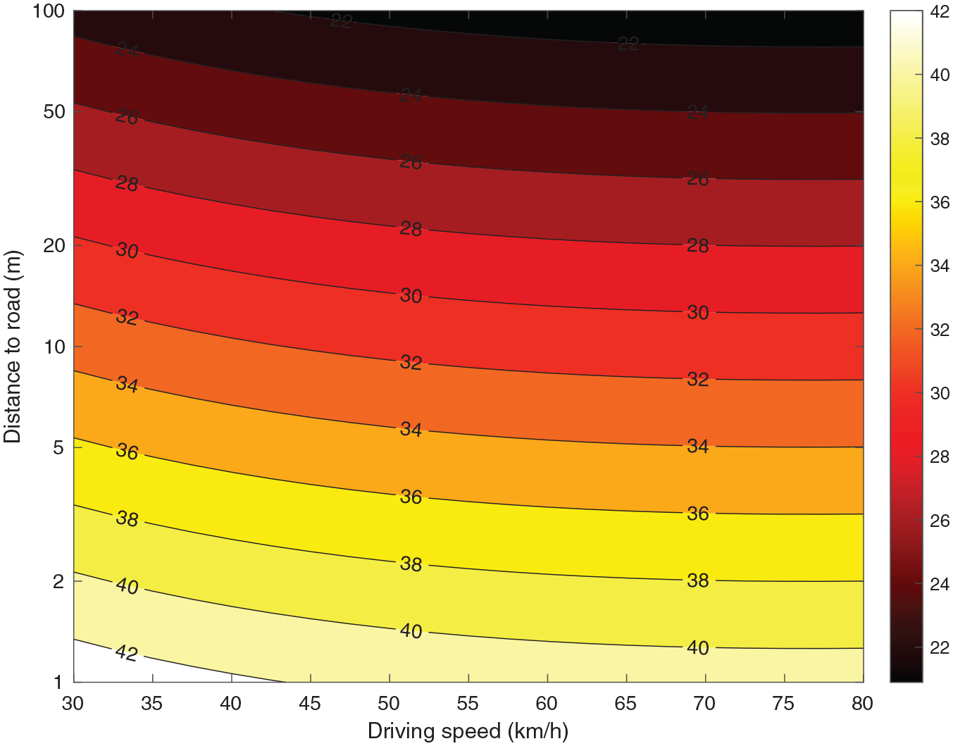
The calculated A-weighted exposure level outdoors, in front of the facade, is displayed in Figure 8 for the ranges in driving speeds of 30–80 km/h and in road-to-facade distance L of 1−100 m. (It could be noted that the results for the smallest values of L, of a few meters, are not relevant for realistic conditions.) It can be seen that the overall trend is that the exposure level increases with driving speed.

Figure 8.

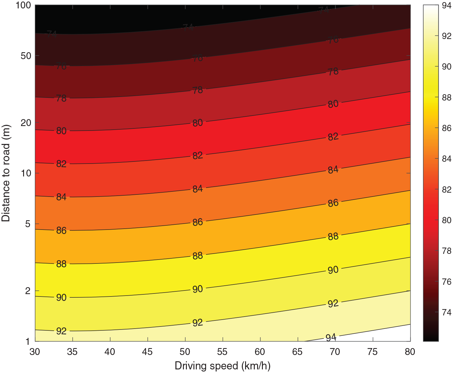
Calculated A-weighted exposure level outdoors, in front of the facade, for driving speed v in the range 30–80 km/h and distance L in the range 1–100 m.

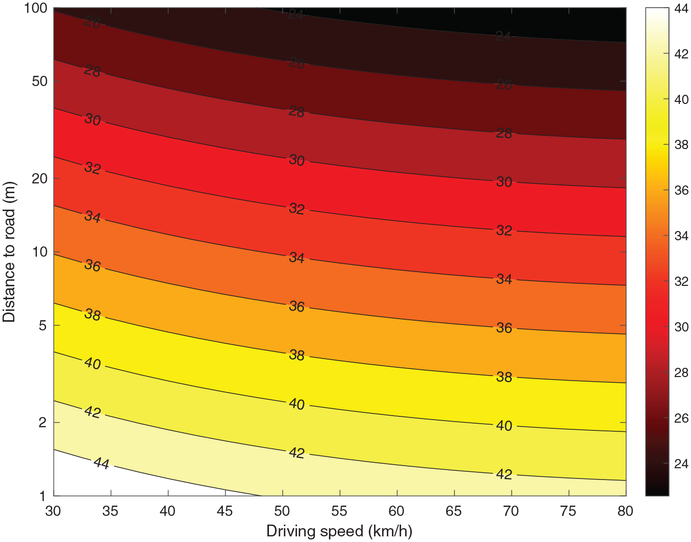
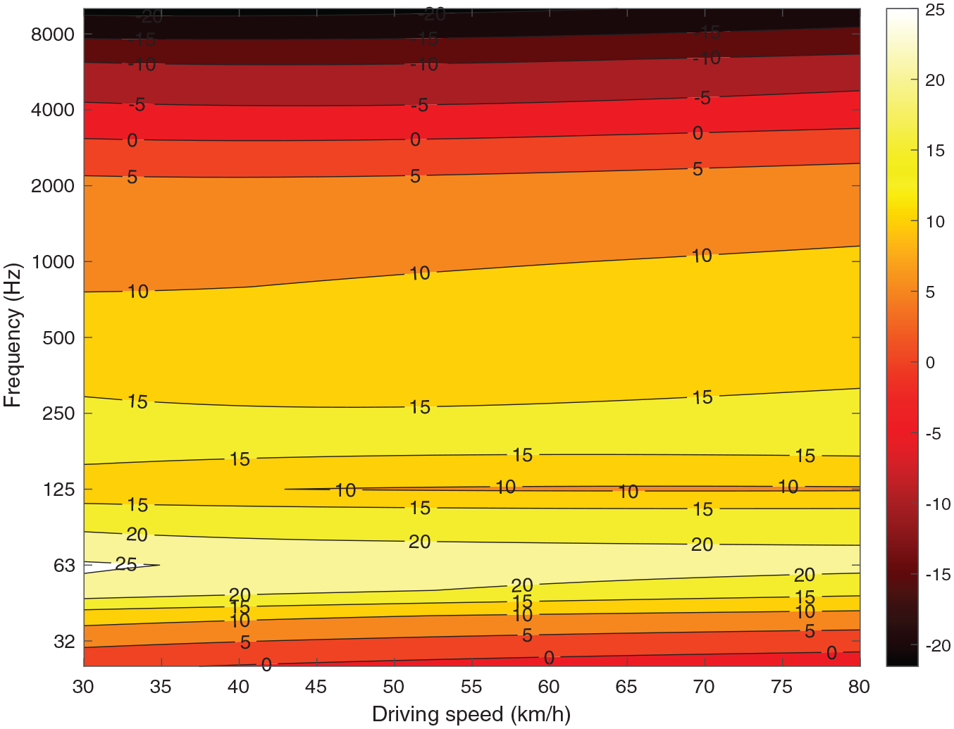
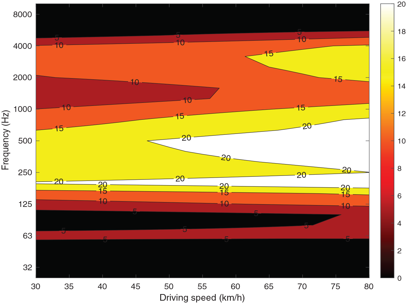
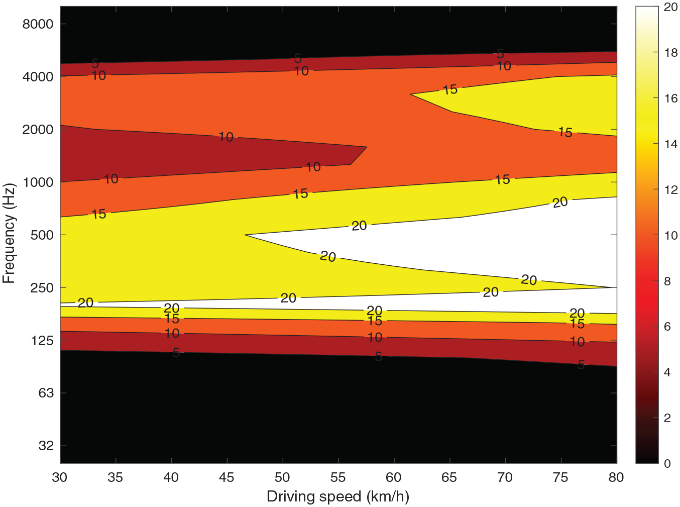
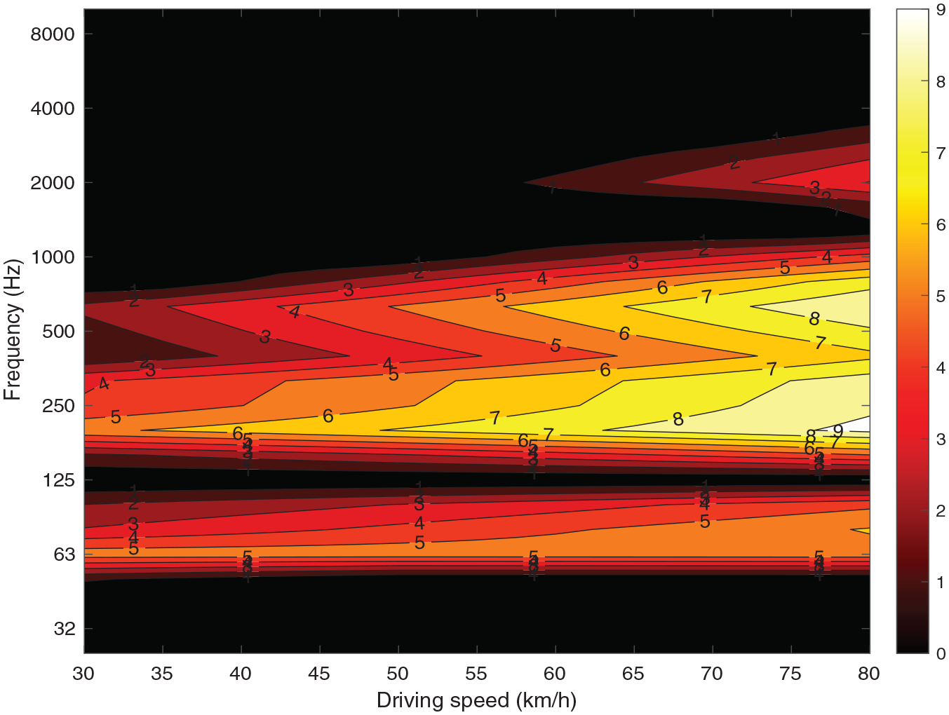
In Figures 9 to 12 the corresponding indoor exposure levels are displayed for the four facade cases. Here it can be seen, contrary to outdoors, that the exposure level may decrease substantially with driving speed, most clearly seen for the soundproof window, that is, in Figures 10 and 12. For the lightweight facade with soundproof window (Figure 10) a decrease of 3 dB takes place when the speed is increased from 30 to 80 km/h, for a distance to road of 10–30 m. Hence, the contribution of a vehicle pass-by to the equivalent level can increase significantly if the driving speed is reduced. This may seem counterintuitive but is due to the small values of the speed coefficients (b-coefficients) of the propulsion noise at low frequencies (as seen in Figure 1), which means that the low-frequency sound power is not decreasing significantly when the sound speed is lowered. This effect is combined with the spectral filtering due to the facade, which increases the relative influence of the corresponding low-frequency components on the total A-weighted exposure level indoors. Figures 13 to 16 displays further details behind this effect where the contribution is shown as function of frequency and of driving speed for a fixed road distance of L = 20 m. One can see that the contribution is accentuated at around 200 Hz when the ordinary window is used (Figures 13 and 15) whereas it is accentuated at around 63 Hz when the soundproof window is used (Figures 14 and 16), most prominently for the steel facade (Figure 14) which allows more sound transmission at these frequencies compared with the concrete facade. And at around 63 Hz one can see how the contribution to the exposure level increases for lower driving speeds in the four figures. (In Figures 13, 14 and 16, looking at the results at around 63 Hz as function of driving speed, one can see that the level is above 25 dB(A) for the lower driving speeds whereas it is below 25 dB(A) for the higher driving speeds; for Figure 14, the same holds but above/below 20 dB(A).)

Figure 9.

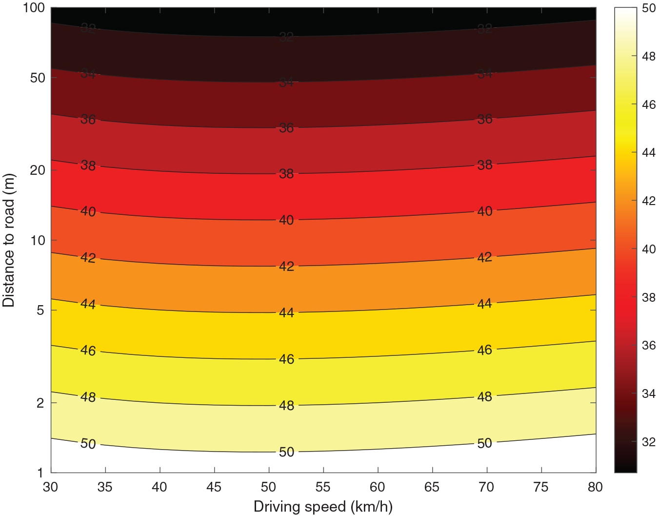
Indoor exposure level (dBA) for facade case 1: lightweight steel facade with ordinary window.

Figure 10.

Indoor exposure level (dBA) for facade case 2: lightweight steel facade with soundproof window.

Figure 11.

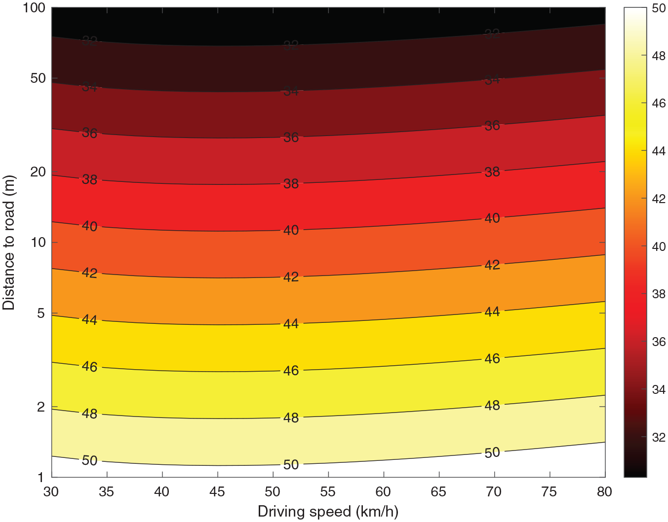
Indoor exposure level (dBA) for facade case 3: concrete facade with ordinary window.

Figure 12.

Indoor exposure level (dBA) for facade case 4: concrete facade with soundproof window.

Figure 13.

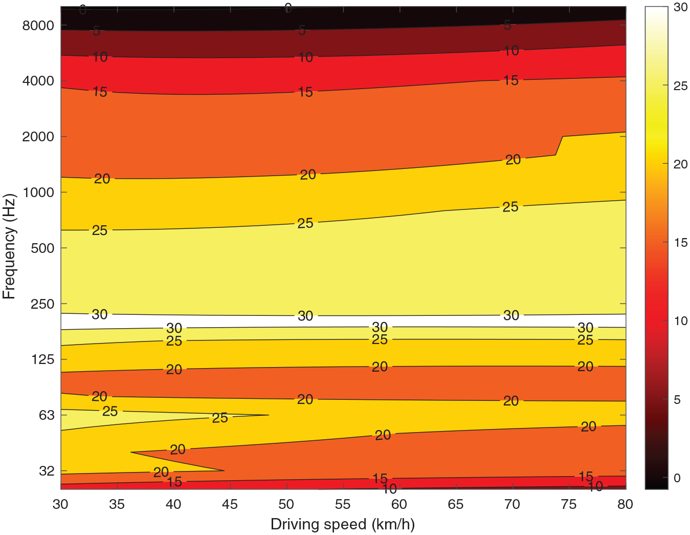
Results for the same situation as for Figure 9, plotted as A-weighted level as function of frequency and of driving speed for a fixed road distance of L = 20 m.

Figure 14.

Results for the same situation as for Figure 10, plotted as A-weighted level as function of frequency and of driving speed for a fixed road distance of L = 20 m.

Figure 15.

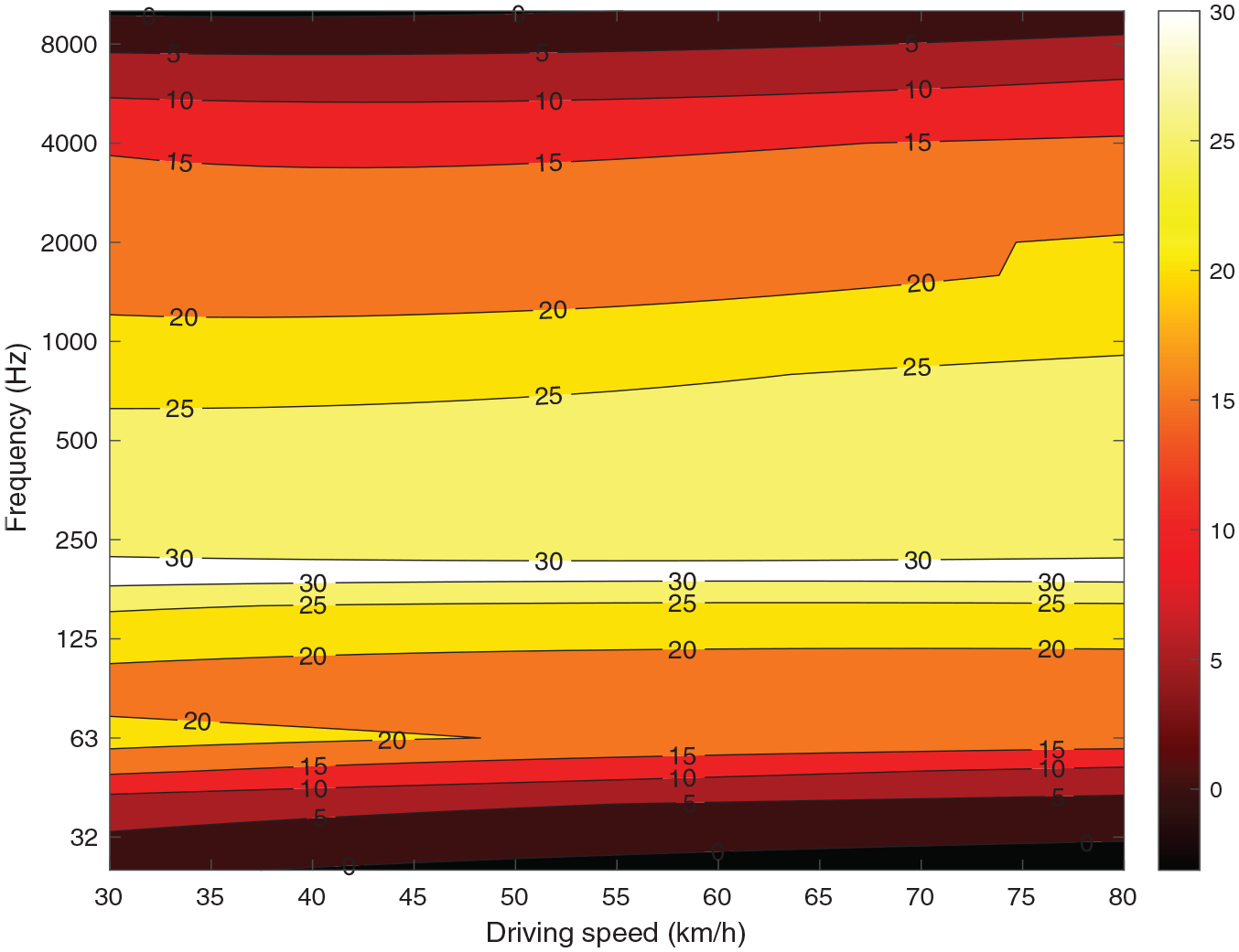
Results for the same situation as for Figure 11, plotted as A-weighted level as function of frequency and of driving speed for a fixed road distance of L = 20 m.

Figure 16.

Results for the same situation as for Figure 12, plotted as A-weighted level as function of frequency and of driving speed for a fixed road distance of L = 20 m.

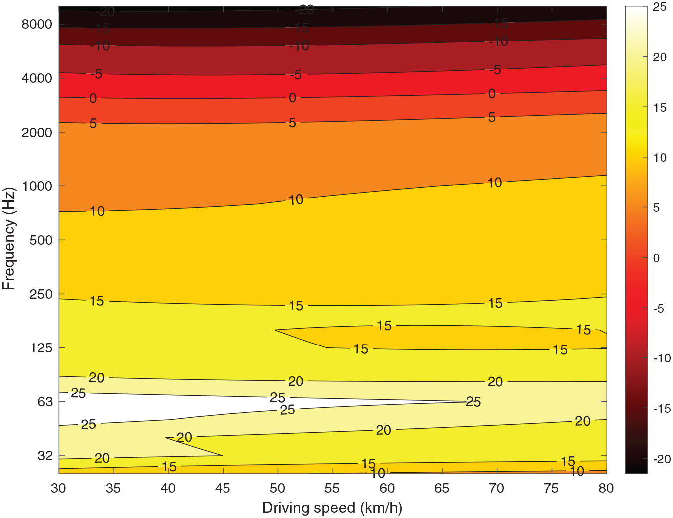
To assess the relevance of the situations selected for the plots in Figures 13 to 16, the corresponding peak levels during pass-by are checked against the hearing threshold. This is presented in Figures 17 to 20 where excess level is plotted, that is, how much the peak level exceeds the hearing threshold. It can be seen that for a road distance of L = 20 m, the pass-by peak level exceeds the hearing threshold for all four facade cases, whereby there is a large possibility for the pass-by events to be audible; hence also for shorter distance to road than 20 m. For some situations with these kinds of events, masking might be provided by other, steady noises indoors, for example, due to ventilation, as indicated by low-frequency equivalent level guideline values. However, for decreased distance between housing and road, the probability of audible pass-by events will increase.

Figure 17.

Results for the same situation as for Figure 13. Plotted is the amount (in dB) with which the peak level exceeds the hearing threshold, as function of frequency and of driving speed for a fixed road distance of L = 20 m. (Black colour means that the peak level is below the hearing threshold.).

Figure 18.

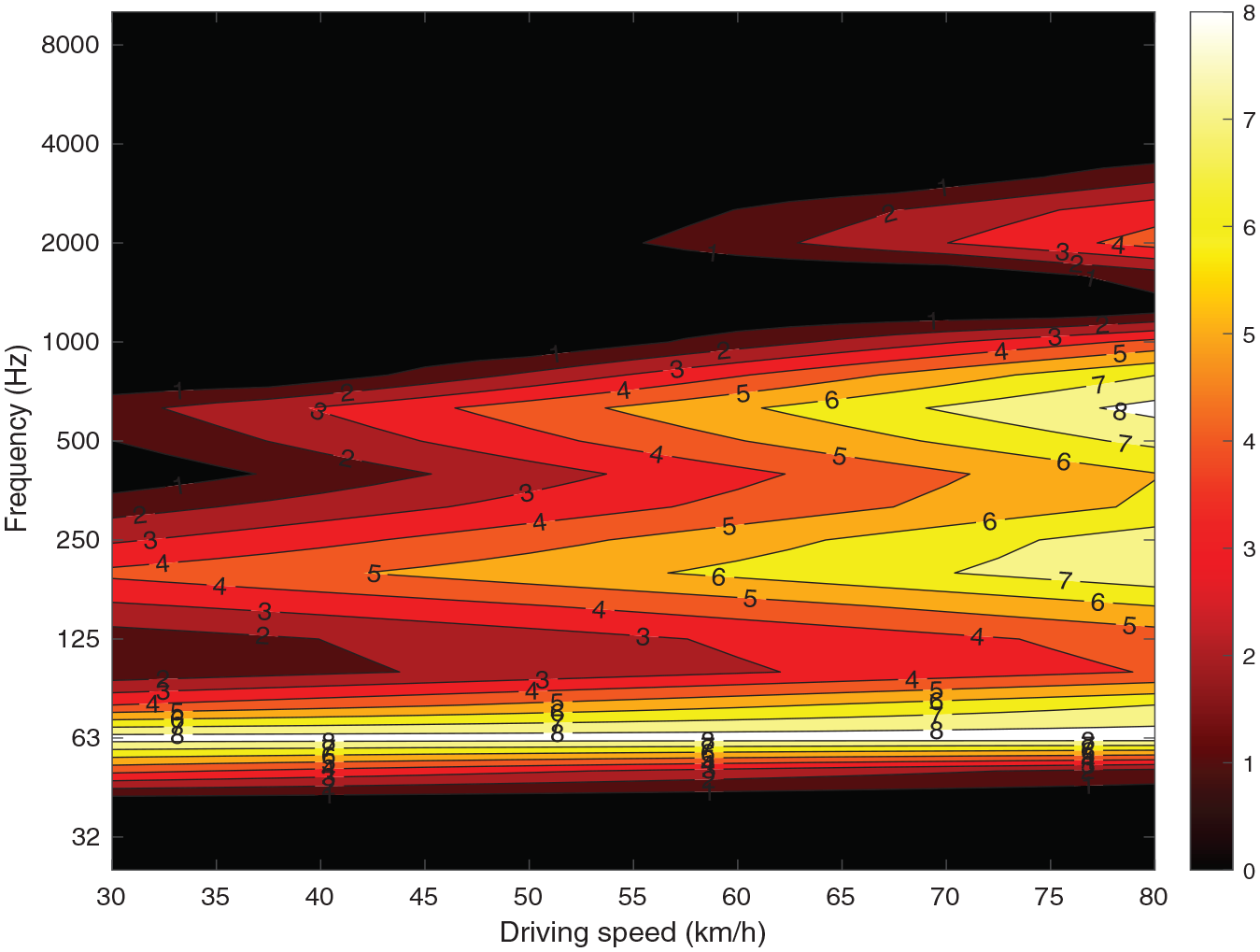
Results for the same situation as for Figure 14. Plotted is the amount (in dB) with which the peak level exceeds the hearing threshold, as function of frequency and of driving speed for a fixed road distance of L = 20 m. (Black colour means that the peak level is below the hearing threshold.).

Figure 19.

Results for the same situation as for Figure 15. Plotted is the amount (in dB) with which the peak level exceeds the hearing threshold, as function of frequency and of driving speed for a fixed road distance of L = 20 m. (Black colour means that the peak level is below the hearing threshold.).

Figure 20.

Results for the same situation as for Figure 16. Plotted is the amount (in dB) with which the peak level exceeds the hearing threshold, as function of frequency and of driving speed for a fixed road distance of L = 20 m. (Black colour means that the peak level is below the hearing threshold.).

Conclusion

The paper presents an investigation of low-frequency noise indoors due to road traffic, based on modelling of simple but realistic examples, using existing source strength models and facade reduction indices utilising measurement data for a lightweight steel facade, a heavy concrete facade, an ordinary double-glazed window and a triple-glazed (soundproof) window made for high noise reduction. The results are divided in two main parts. From the results of the first part, about the audibility of individual pass-by events, it can be concluded that new housing built close to a busy road risks to be detrimental for wellbeing due to poor indoor sound environments, despite the use of high-quality windows and facade walls: Low-frequency pass-by noise may be audible and the number of pass-by events may be disturbingly large, while still all applicable noise regulations are fulfilled. Furthermore, it was shown that the low-frequency components of heavy road vehicles may dominate the A-weighed level indoors.

From the results of the second part, about exposure level dependence on driving speed and distance to road, it was shown that the low-frequency speed dependence of the heavy vehicle source strength, in combination with the facade sound insulation, may cause the equivalent indoor noise level to increase when the driving speed is reduced. Concerning the exposure levels, accentuated results were shown at around 200 Hz when the ordinary window was used and at around 63 Hz when the soundproof window was used, most prominently so for the lightweight facade.

Although the situation we modelled here is for a smaller apartment, similar conclusions would apply to larger apartments. And even for lower traffic flows or lower proportion of heavy vehicles, it may be disruptive if many passages are audible during the hours one wants to sleep.

That this example study demonstrates the risk of a large number of audible passages of road vehicles at night, and thus a high risk of disturbance, should call for caution in urban densification where new homes are built near to roads with large flows of traffic.

An additional factor in this context is that the difference in level between an audible sound and a disturbing sound is smaller for sounds that are dominated by low frequencies, so only a small change may be required for a sound to go from being barely audible to being clearly disturbing.

If a very high facade insulation is not afforded, it might be preferable to build in less noisy areas, either to densify outside the inner city or create new attractive areas. Both of these alternatives can often be combined with proximity to natural environments, which may have high attraction value if advantage is taken of the natural environment’s soundscape potential.

It should be pointed out that electrification of heavy vehicles to a large extent can provide a remedy to the detrimental issues pointed out here. However, there is still a long way to go until we reach a good sound environment, as can be highlighted by the difference between current limit values and the ones suggested by WHO.

For future work, it would be valuable to use real-life measured data to confirm the modelled results reported here.