Analysis of the sound insulation performance of periodic wall structures by a virtual acoustic laboratory

Abstract

The propagation of acoustic waves in periodic structures, also known as phononic crystals or PCs, is prohibited in certain frequency ranges, which are referred to as the frequency band-gaps. The existence, the location and the width of the frequency band-gaps are mainly determined by the geometrical parameters and the material properties of the PCs. In this work, a virtual acoustic laboratory based on a fully coupled fluid-structure interaction (FSI) model is developed to determine the sound insulation capacity of one-dimensional (1D) and two-dimensional (2D) periodic walls. The FSI model is discretized using the frequency-domain spectral element method (FDSEM), which is an advanced finite element method (FEM) using special high-order shape functions. Following the guidelines of the ISO10140, the setup of the developed FSI model allows us to take into account the essential physical phenomena, especially the interaction of the wall structure with the fluid domains (air). The FSI model based on the FDSEM increases the computational efficiency and accuracy in comparison with the standard FEM. Several numerical examples will be presented and discussed to show that the designed periodic walls in certain frequency ranges within the band-gaps may exhibit much better sound insulation capabilities than monolithic walls.

Introduction

A wall construction, used in civil engineering, requires good acoustic insulation to protect people from the harmful impact of noise exposure or to protect sensitive measurement instrumentation and equipment in laboratories and industrial manufacturing. Recently, periodic structures have received more attention for their far superior acoustic protection capabilities in a range of applications. It is widely known ¹ that the acoustic/elastic wave propagation in periodic structures can be severely hindered in certain frequency ranges due to the scattering effects or the local resonances. The frequency range, in which the wave propagation is prohibited, is referred to as the band-gap, and the periodic structures are known as the phononic crystals (PCs) or frequently also metamaterials (MMs). Extensive works have been done in recent years regarding the applications of PCs, especially acoustic/elastic wave devices, sound isolation and vibration suppression, etc., but very little studies are devoted to the potential use of PCs in building acoustics.

This work aims to determine the sound reduction index (SRI) of walls composed of periodic substructures via a virtual laboratory. The virtual laboratory uses a theoretical model for the description of the fluid-structure interaction (FSI) and follows the guidelines of the ISO 10140. ² In this model, the interactions between the air in the source room, the wall specimen, and the air in the receiving room are taken into account. While several methods have been developed for the analytical and numerical determination of the acoustic wave transmission loss in layered wall structures of rather simple geometry, such as the transfer matrix method or the statistical energy analysis,^3,4 only the FSI model can consider the mostly important physical phenomena, such as the strong coupling between the fluid domain and the structure, and has very few limitations regarding the boundary conditions, the geometry and the material properties. This increases the reliability and flexibility of the calculation and allows for a realistic numerical simulation and comparison with experimental measurements.

In the past, several studies used the FSI model to determine the acoustic wave transmission loss in structural panels and walls. The calculation in the high-frequency ranges needs a great deal of computational resources. Therefore, most previous studies only focused on the low-frequency range.^5,6 Clasen and Langer examined the influence of flanking transmission and approximated the wall structure by beam elements. ⁷

More recently, Arjunan et al.^8,9 used a finite element method (FEM) model to determine the sound transmission loss in double panels and del Coz Díaz et al. ¹⁰ used a two-dimensional (2D) model to investigate the sound transmission loss in brick walls in the high-frequency range. Studies about the use of the FSI model and the influences of several effects, such as the mounting conditions or the absorption characteristics of the virtual laboratory, have also been conducted^11,12 and the three-dimensional (3D) geometry of the laboratory was considered to reduce the influences of the eigenmodes.^13,14 The FSI model is still very rarely used to examine the sound insulation capabilities of a wall structure and the related literature is rather limited. One of the possible reasons for this is probably the relatively simple setup of the standard wall structures used in building acoustics and the wide range of possible analytical and numerical methods to predict their behavior. However, for the examination of complex geometry, boundary conditions and material properties, such as periodic walls and the sophisticated interference phenomena which arise, a detailed FSI model is necessary.

To improve the accuracy and the efficiency of the computational simulation in the virtual laboratory, the FSI model in this work is treated numerically using the spectral element method (SEM), which is an advanced FEM using special high-order shape functions. The SEM was developed by Patera in 1984 to solve some problems in computational fluid dynamics. ¹⁵ Later, it was also applied to a wide variety of engineering problems, for example, wave propagation in functionally graded materials, ¹⁶ structural health monitoring, ¹⁷ seismology ¹⁸ and many other fields. The general superiority of the SEM in analyzing the wave propagation problems with high accuracy was studied in many previous works and also compared to other spectral methods.^19–22 However, to the best knowledge of the authors, no previous works using the SEM to calculate the SRI of a wall structure based on the FSI model have been yet reported in literature.

This paper has two main purposes. The first one is to develop a virtual acoustic laboratory to test and predict the sound insulation performance of wall structures via a FSI model. The SEM is adopted for solving the theoretical model of the virtual laboratory and its efficiency for calculating the SRI with different accuracy levels is examined. The second purpose is to use the virtual laboratory based on the FSI model and the SEM to examine the sound insulation capabilities of periodically structured walls. While some simple methods like the transfer matrix method and the stiffness matrix method are able to predict the SRI of one-dimensional (1D) layered walls, they can not recover certain physical phenomena that occur in periodically layered walls. For 2D and 3D arbitrary geometry, there exists no theoretical and rigorous model to accurately predict the SRI and a FSI model is thus needed.

The paper is structured as follows. In the following section, we present the governing equations for the FSI model and its discretization in the framework of the SEM. The setup of the virtual laboratory is described and validated by comparison with measured data for simple wall structures. Furthermore, a brief description of the basic principle of periodic structures is given. Afterward, we discuss the accuracy and the efficiency of the FSI model and demonstrate the advantages of the SEM. Subsequently, the main results of the paper are presented, where we examine several 1D layered and 2D periodically structured walls and show their superior sound insulation capabilities in the band-gap. The influences of the material parameters and the geometrical configurations of the wall structures are investigated in detail, and a comparison between the theoretical predictions by the dispersion diagrams of the unit-cells and the actual frequency responses in term of the SRI curves of the respective periodic wall structures is shown. At the end, we conclude the paper and summarize the essential findings.

Descriptions of the FSI model, the SEM and the virtual acoustic laboratory

Governing equations and the FSI model

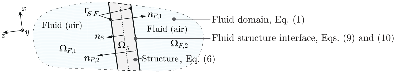
In the experimental determination of the sound reduction index of a wall, a measurement laboratory is used. Two rooms, the source room and the receiving room, are divided by the wall specimen. In the source room, the placed loudspeakers emit acoustic waves at varying frequencies. The resulting pressure distribution excites the wall specimen, which then vibrates and induces a pressure distribution in the receiving room. The sound pressure is measured using microphones and from the difference between the sound pressure levels in the source room and the receiving room, the transmission loss is obtained. In this work, this process is simulated by a theoretical model describing the fluid-structure interaction (see Figure 1).

Figure 1.

Definitions of the normal vectors and the fluid and structural domains in the FSI model.

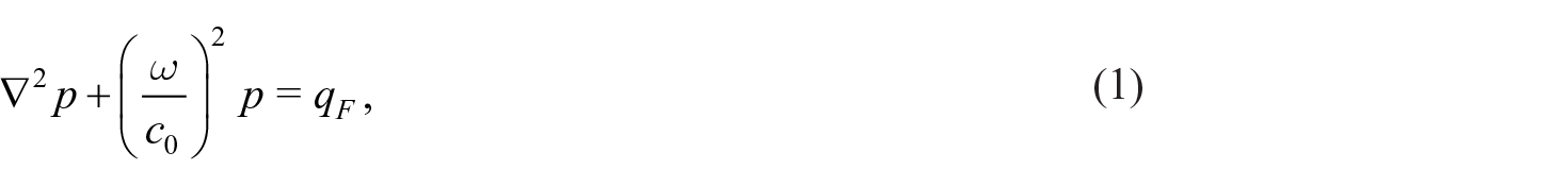
The governing equation for the fluid or air domain is the following Helmholtz equation for a compressible inviscid fluid:

$${\nabla }^{2}p+{\left(\frac{\omega }{c_0}\right)}^{2}p=q_F,$$

(1)

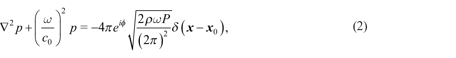
with the pressure $p,$ the angular frequency $\omega ,$ the speed of sound $c_0,$ the source $q_F$ and the nabla operator ${\nabla }^T=\left[\begin{array}{ccc}\frac{\partial }{\partial x}& \frac{\partial }{\partial y}& \frac{\partial }{\partial z}\end{array}\right].$ In equation (1) and throughout the paper, the common time-harmonic term $e^{i\omega t}$ is omitted for the sake of brevity. A monopole sound source is used as a representation of a loudspeaker in a test laboratory, which satisfies the equation

$${\nabla }^{2}p+{\left(\frac{\omega }{c_0}\right)}^{2}p=-4\pi e^{i\varphi }\sqrt{\frac{2\rho \omega P}{{\left(2\pi \right)}^2}}\delta \left(\mathit{x}-{\mathit{x}}_0\right),$$

(2)

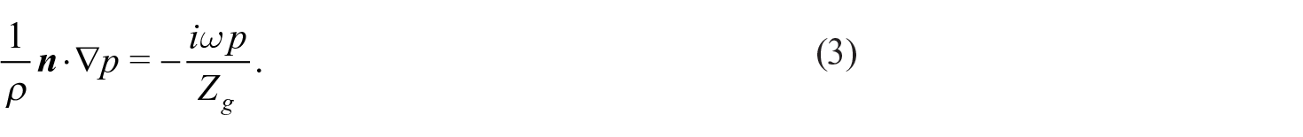
with the phase angle $\varphi ,$ the power of the sound source $P$ and the Dirac-delta function $\delta (\mathit{x}-{\mathit{x}}_0)$ . The following impedance boundary condition is used for defining a specific impedance $Z_g$ at a boundary:

$$\frac{1}{\rho }\mathit{n}\cdot \nabla p=-\frac{i\omega p}{Z_g}.$$

(3)

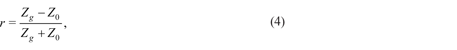
Here, $\mathit{n}$ is the outward normal vector on the boundary and $i$ is the imaginary unit. With the impedance boundary condition it is possible to assign a specific reflection coefficient $r$ or absorption coefficient $\alpha$ to a surface. They are related to the impedance by

$$r=\frac{Z_g-Z_0}{Z_g+Z_0},$$

(4)

and

$$\alpha =1-r^2,$$

(5)

with the characteristic surface impedance $Z_g$ of the structure and the characteristic impedance of air $Z_0.$ For a normal wave incidence $Z_g=\rho c$ and $Z_0={\rho }_0{c}_0,$ while for an oblique wave incidence $Z_g=\rho c/\cos \theta$ and $Z_0={\rho }_0{c}_0/\cos {\theta }_0.$ Here, ${\theta }_0$ is the angle of the wave incidence and $\theta$ is the angle of the transmitted wave, which are related by the Snell’s law $c_0\sin \theta =c\sin {\theta }_0$ or $\sin \theta /\sin {\theta }_0=c/c_0.$ Then, equation (4) is also valid for a random wave incidence by properly taking the statistical average of the corresponding quantities, under the assumption of a perfect interface described by the impedance boundary condition given in equation (3). The considered wall specimen is described by the equations of motion for a homogenous, isotropic and linear elastic continuum in the frequency-domain as

$${\tilde{\nabla }}^T{\sigma }_S+\mathit{f}=-{\rho }_S{\omega }^2\mathit{u},$$

(6)

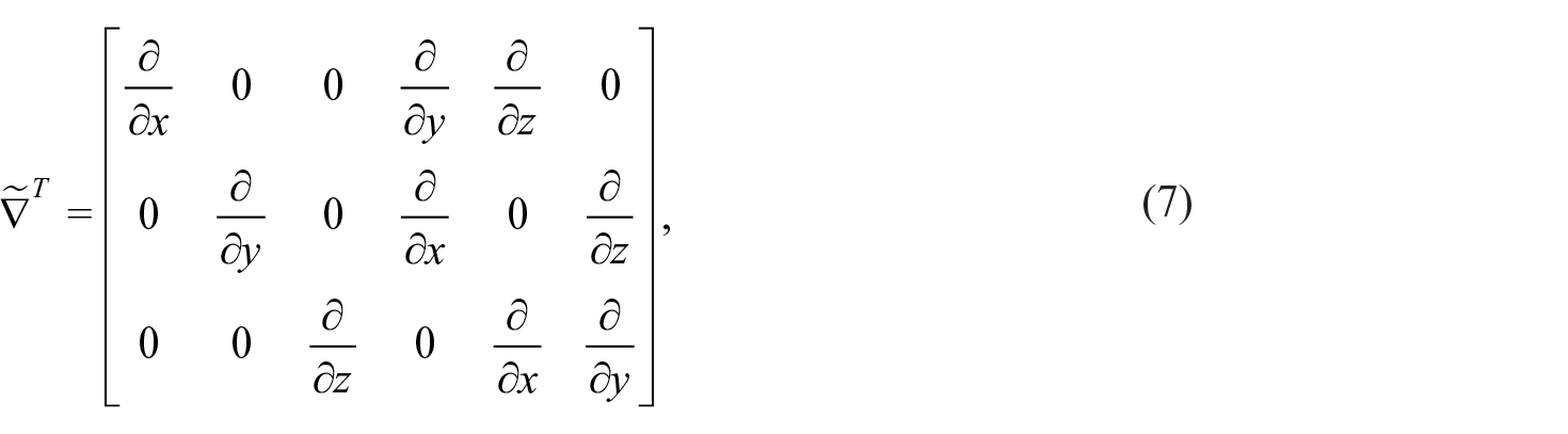
with

$${\tilde{\nabla }}^T=\left[\begin{array}{cccccc}\frac{\partial }{\partial x}& 0& 0& \frac{\partial }{\partial y}& \frac{\partial }{\partial z}& 0\\ 0& \frac{\partial }{\partial y}& 0& \frac{\partial }{\partial x}& 0& \frac{\partial }{\partial z}\\ 0& 0& \frac{\partial }{\partial z}& 0& \frac{\partial }{\partial x}& \frac{\partial }{\partial y}\end{array}\right],$$

(7)

the stress vector ${\sigma }_S^T={\left[{\sigma }_{xx}{\sigma }_{yy}{\sigma }_{zz}{\sigma }_{xy}{\sigma }_{xz}{\sigma }_{yz}\right]}^T,$ the body force vector $\mathit{f},$ the mass density of the structure ${\rho }_S$ and the displacement vector $u.$ In the 2D problems considered in this work, the solid wall structure is assumed to be under the plain strain condition. The structural damping is considered by using a complex Young’s modulus $E$ ²³ with the isotropic loss factor $\eta$ as

$$E\to E\left(1+i\eta \right).$$

(8)

This method does not implicitly take the frequency dependence of the material behavior into account, but will be still used, since the necessary material coefficients for more sophisticated models are not known for the materials under consideration and due to its simplicity for use. Nevertheless, the method delivers a good approximation for structural attenuation.

The pressures in the source room ${\Omega }_{F_1}$ and the receiving room ${\Omega }_{F_2}$ result in a force resultant on the boundaries of the structure ${\Omega }_S$ and the vibrations of the structure induce an acoustic pressure field in the fluid domains. The reciprocal influence between the structure and the fluid is referred to as strong fluid-structure interaction or coupling, which is necessary to be taken into account for the accurate determination of the sound insulation capabilities of walls in building acoustics. ²⁴ The fluid and structural domains are shown in Figure 1. Their interaction is described by the following continuity and equilibrium conditions on the fluid-structure interfaces:

$${{\mathit{u}}_S\mathit{n}|}_{{\Gamma }_{S,F}}={{\mathit{u}}_F\mathit{n}|}_{{\Gamma }_{S,F}},$$

(9)

and

$$\mathit{t}=-p{\mathit{n}}_S=p{\mathit{n}}_F,$$

(10)

where $\mathit{t}$ is the Cauchy stress vector. The definition of the normal vectors is given in Figure 1.

Numerical discretization by the SEM

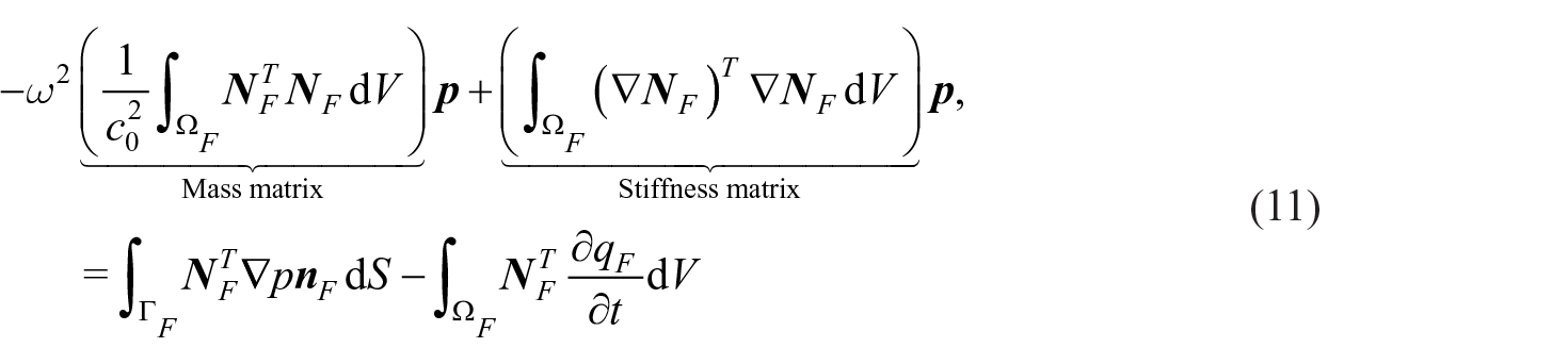
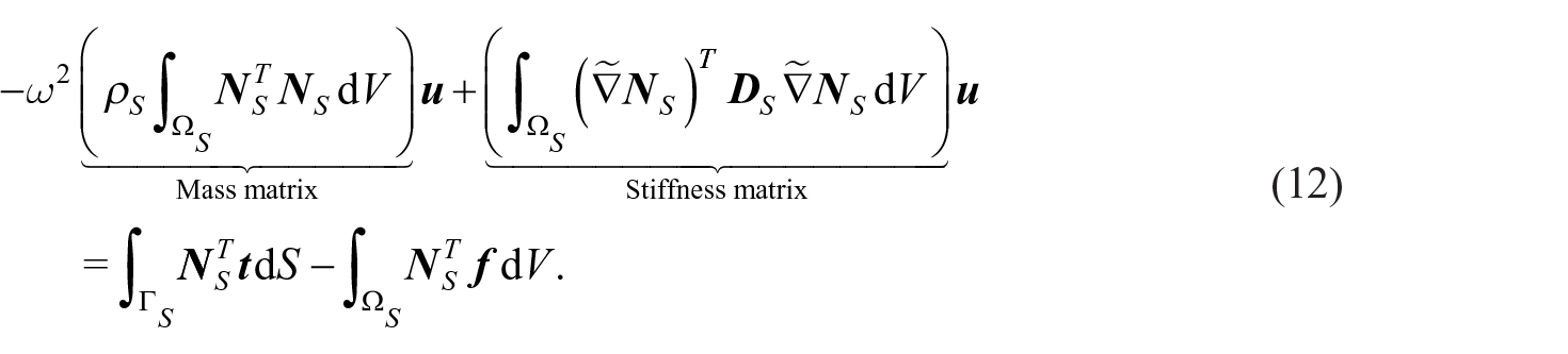
Using the weak-form formulation or the Galerkin method, the boundary value problem under consideration can be recast into a discretized form by approximating the pressure field as $p(\mathit{x})={\mathit{N}}_F\mathit{p}.$ Here, ${\mathit{N}}_F$ is the vector of the shape functions and $\mathit{p}$ is the nodal pressure vector. The displacement field is approximated by $\mathit{u}(\mathit{x})={\mathit{N}}_S\mathit{u}$ with the matrix of the shape functions ${\mathit{N}}_S$ and the nodal displacement vector $\mathit{u}.$ For the sake of conciseness we refer to Pozrikidis ²⁵ for a detailed explanation of the Galerkin method. The discretized linear system of algebraic equations for equation (1) then is

$$\begin{array}{l}-{\omega }^2\underset{\begin{array}{c}\mathrm{Mass}\mathrm{matrix}\end{array}}{\underbrace{\left(\frac{1}{c_0^2}{\int }_{{\Omega }_F}{\mathit{N}}_F^T{\mathit{N}}_F\mathrm{d}V\right)}}\mathit{p}+\underset{\begin{array}{c}\mathrm{Stiffness}\mathrm{matrix}\end{array}}{\underbrace{\left({\int }_{{\Omega }_F}{\left(\nabla {\mathit{N}}_F\right)}^T\nabla {\mathit{N}}_F\mathrm{d}V\right)}}p,\\ ={\int }_{{\Gamma }_F}{\mathit{N}}_F^T\nabla p{\mathit{n}}_F\mathrm{d}S-{\int }_{{\Omega }_F}{\mathit{N}}_F^T\frac{\partial q_F}{\partial t}\mathrm{d}V\end{array}$$

(11)

and for equation (6) we get

$$\begin{array}{l}-{\omega }^2\underset{\begin{array}{c}\mathrm{Mass}\mathrm{matrix}\end{array}}{\underbrace{\left({\rho }_S{\int }_{{\Omega }_S}{\mathit{N}}_S^T{\mathit{N}}_S\mathrm{d}V\right)}}\mathit{u}+\underset{\begin{array}{c}\mathrm{Stiffness}\mathrm{matrix}\end{array}}{\underbrace{\left({\int }_{{\Omega }_S}{\left(\tilde{\nabla }{\mathit{N}}_S\right)}^T{\mathit{D}}_S\tilde{\nabla }{\mathit{N}}_S\mathrm{d}V\right)}}\mathit{u}\hfill \\ ={\int }_{{\Gamma }_S}{\mathit{N}}_S^T\mathit{t}\mathrm{d}S-{\int }_{{\Omega }_S}{\mathit{N}}_S^T\mathit{f}\mathrm{d}V.\hfill \end{array}$$

(12)

Here, ${\mathit{D}}_S$ is the elasticity matrix (see e.g. Pozrikidis ²⁵ for a definition of the elasticity matrix and the stress-strain relation). The terms for the element mass matrices and element stiffness matrices are labeled in equations (11) and (12). After assembly according to the standard procedure of the FEM, we finally get the following system of linear algebraic equations for the fluid domain

$$\left({\mathit{K}}_F-{\omega }^2{\mathit{M}}_F\right)\mathit{p}={\mathit{F}}_F,$$

(13)

and for the structural domain

$$\left({\mathit{K}}_S-{\omega }^2{\mathit{M}}_S\right)\mathit{u}={\mathit{F}}_S,$$

(14)

where $\mathit{K}$ is the stiffness matrix and $\mathit{M}$ is the mass matrix, for the fluid domain denoted by the subscript $\mathit{F},$ and for the structural domain denoted by the subscript $S.$ $F$ on the right hand side of equations (11) and (12) stands for the force or loading vectors of the fluid and structural domains, respectively.

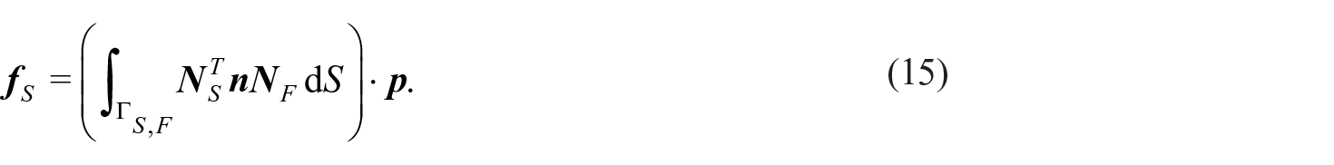
The interaction between the fluid and the structural domains is considered by the coupling conditions. Using equation (10) in the first part of the right hand side of equation (12) leads to the approximation of the acoustic pressure on the boundary of the structural domain as

$${\mathit{f}}_S=\left({\int }_{{\Gamma }_{S,F}}{\mathit{N}}_S^T\mathit{n}{\mathit{N}}_F\mathrm{d}S\right)\cdot \mathit{p}.$$

(15)

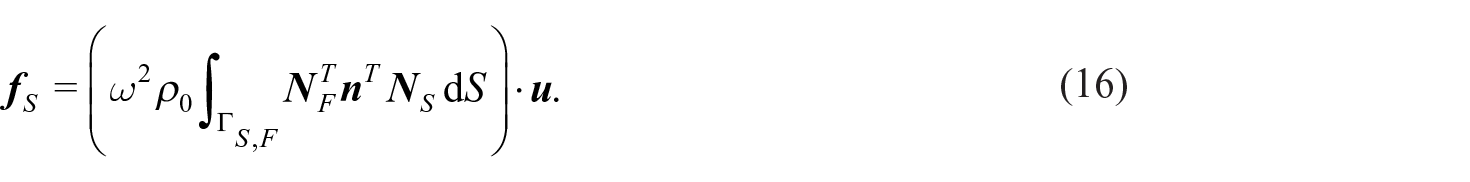
The dynamic displacements on the boundary of the fluid domain can be approximated by substituting equation (9) with $\nabla p={\omega }^2{\rho }_0{\mathit{u}}_F$ in the first part of the right hand side of equation (11), which leads to

$${\mathit{f}}_S=\left({\omega }^2{\rho }_0{\int }_{{\Gamma }_{S,F}}{\mathit{N}}_F^T{\mathit{n}}^T{\mathit{N}}_S\mathrm{d}S\right)\cdot \mathit{u}.$$

(16)

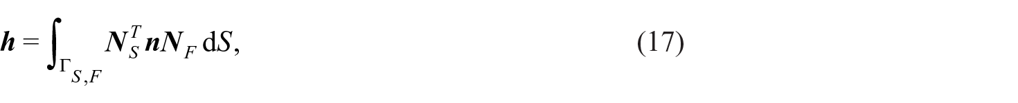
Since only the displacement component in the normal direction of the structure causes an acoustic pressure in the fluid, the shape functions not corresponding to this direction have to be set to zero in equations (15) and (16). After introducing the element coupling matrix

$$\mathit{h}={\int }_{{\Gamma }_{S,F}}{\mathit{N}}_S^T\mathit{n}{\mathit{N}}_F\mathrm{d}S,$$

(17)

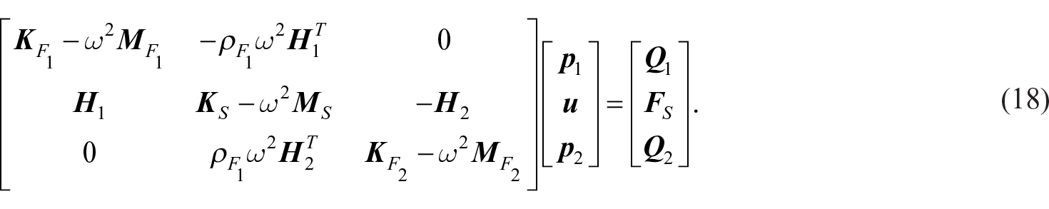
and assembling the element coupling matrices to the global coupling matrix $\mathit{H}$ the linear system of the resulting algebraic equations can then be written as

$$\left[\begin{array}{ccc}{\mathit{K}}_{F_1}-{\omega }^2{\mathit{M}}_{F_1}& -{\rho }_{F_1}{\omega }^2{\mathit{H}}_1^T& 0\\ {\mathit{H}}_1& {\mathit{K}}_S-{\omega }^2{\mathit{M}}_S& -{\mathit{H}}_2\\ 0& {\rho }_{F_1}{\omega }^2{\mathit{H}}_2^T& {\mathit{K}}_{F_2}-{\omega }^2{\mathit{M}}_{F_2}\end{array}\right]\left[\begin{array}{c}{\mathit{p}}_1\\ \mathit{u}\\ {\mathit{p}}_2\end{array}\right]=\left[\begin{array}{c}{\mathit{Q}}_1\\ {\mathit{F}}_S\\ {\mathit{Q}}_2\end{array}\right].$$

(18)

This is the discretized FSI model used in this work. We refer to the literature for further details and a more in-depth explanation, for example Sandberg and Ohayon. ²⁶

The introduction of a monopol source, see equation (2), is quite trivial: Since the Delta function has the sifting property ${\int }_{a-\epsilon }^{a+\epsilon }f\left(x\right)\delta \left(x-a\right)\mathrm{d}x=f\left(a\right),$ the term $-4\pi e^{i\varphi }\sqrt{\frac{2\rho \omega P}{{\left(2\pi \right)}^2}}$ can be simply added to the right hand side of equation (18) according to the geometrical position of the source.

The above described coupling procedure is rather straight-forward and easy to implement, but it requires conforming meshes for the fluid domain and the structural domain. If, for instance, different meshes are used for the fluid domain and the structural domain and therefore, the positions of the nodes of the meshes are not identical on the coupling interfaces, other coupling methods are advantageous. Possible approaches include the Consistent Interpolation Method, ²⁷ the Mortar Method ²⁸ or the Localized Lagrange Multipliers Method.^29,30

Shape functions of the SEM

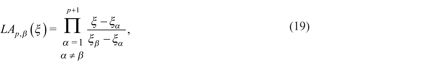
In the SEM, the Lagrange polynomials $LA$ are used as shape functions $\phi ,$ which are defined by

$$L{A}_{p,\beta }\left(\xi \right)=\underset{\underset{\alpha \ne \beta }{\alpha =1}}{\overset{p+1}{\Pi }}\frac{\xi -{\xi }_{\alpha }}{{\xi }_{\beta }-{\xi }_{\alpha }},$$

(19)

where $p$ is the order, ${\xi }_{p+1}$ is the nodal set for the construction of the polynomials, and $\alpha$ and $\beta$ are the node numbers.

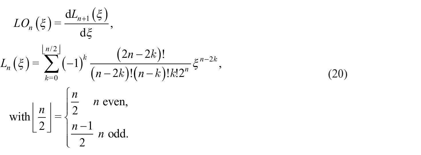
In the conventional FEM, the nodes $\xi$ are evenly distributed (abbreviated by ED), causing the so-called Runge-oscillations at the edges for high orders of $p$ and resulting in a large numerical error of the calculation. The Runge-oscillations can be avoided in the SEM by the distribution of the nodes at the zeros of the Lobatto polynomial $L{O}_{p-1}$ and the edges of the element. This is referred to as the Gauss-Lobatto-Legendre node distribution (abbreviated by GLL). The Lobatto polynomial is defined by

$$\begin{array}{l}L{O}_n\left(\xi \right)=\frac{\mathrm{d}{L}_{n+1}\left(\xi \right)}{\mathrm{d}\xi }\mathrm{,}\\ L_n\left(\xi \right)=\sum _{k=0}^{\lfloor n/2\rfloor }{\left(-1\right)}^k\frac{\left(2n-2k\right)!}{\left(n-2k\right)!\left(n-k\right)!k{!2}^n}{\xi }^{n-2k},\\ \mathrm{with}\lfloor \frac{n}{2}\rfloor =\{\begin{array}{l}\frac{n}{2}n\mathrm{even},\\ \frac{n-1}{2}n\mathrm{odd}\mathrm{.}\end{array}\end{array}$$

(20)

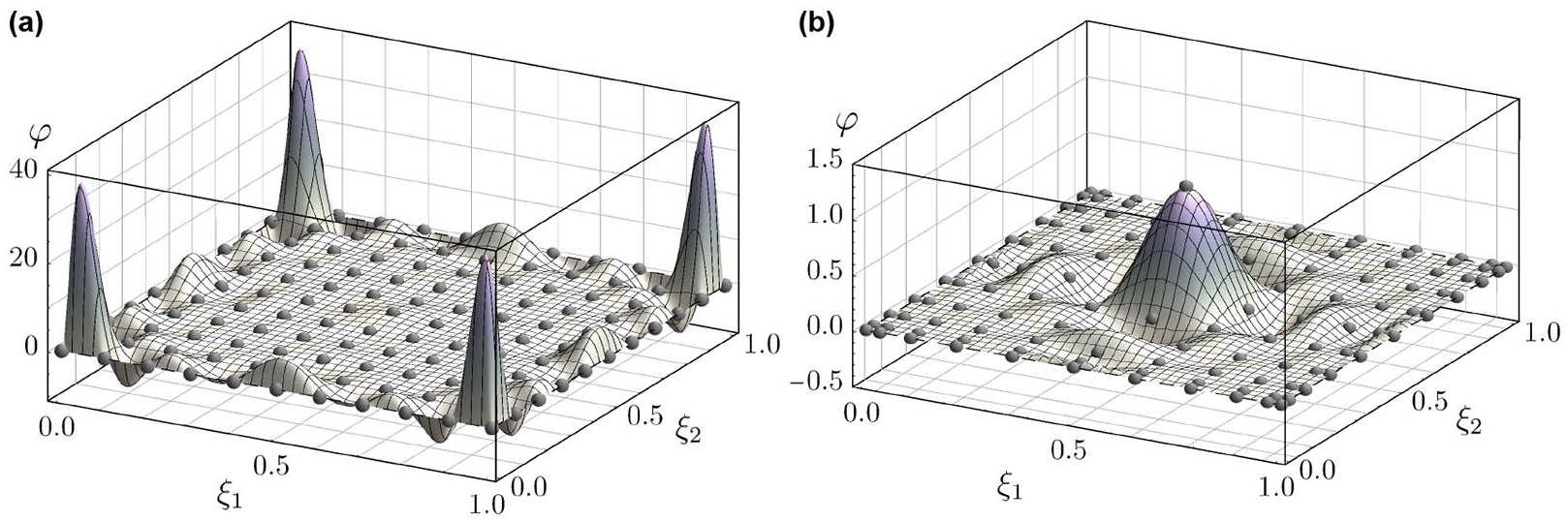
The use of the GLL shape functions leads to a much lower condition number of the linear system of algebraic equations, which allows us to use much higher orders of the shape functions without increasing the numerical error.^25,31 This leads to the spectral convergence of the SEM. In contrast, increasing the number of elements only leads to an algebraic convergence rate. An example for the 2D shape function using the ED node distribution is given in Figure 2(a), which shows the Runge-oscillations at the edges. In Figure 2(b), the GLL node distribution is used, which avoids the oscillations and limits the functional values to unity. The 2D and 3D shape functions can be easily constructed by the product of the one-dimensional (1D) shape functions.

Figure 2.

The 2D shape function $\phi$ for $p=10,$ $\beta =61$ with (a) ED and (b) GLL node distributions.

Another important aspect of the SEM is the possibility of using the Lobatto quadrature for the numerical integration of the element mass matrices in equations (11) and (12). ²⁵ This leads to a perfectly diagonal element mass matrix but also introduces a small error in the calculation. In most practical applications, however, this error is negligible. An exact integration is possible by the use of the Gauss-Legendre quadrature, but this leads to fully occupied element mass matrices.

Virtual acoustic laboratory for the determination of the transmission loss

The measurement of the sound insulation capabilities of a wall structure usually follows some national or international guidelines for the setup of the experimental determination, for example the DIN EN ISO 10140 in Germany, ² to enable a better comparison between different laboratories. The theoretical model in this work follows these guidelines as well, so that the numerical result can, in principle, be compared to the measured sound reduction index (SRI) of a wall specimen. For this reason, we call the model in this work a virtual laboratory. Nevertheless, the measured SRI in different laboratories may differ considerably for the same specimen, especially in the low-frequency range. The reason for this is due to the differences in the sizes of the laboratory, the mounting of the specimen, the absorption characteristics of the laboratory walls, the temperature and humidity of the air, etc. The works of Schmitz et al. ³² and Meier et al. ³³ have shown possible deviations of up to 20 dB in the low-frequency range and 4–8 dB in the high-frequency range for the same specimen, but measured in different laboratories. However, the work of de Melo et al. ³⁴ has demonstrated that, if all material properties, the geometry of the laboratory, and other impact factors are very well known, a numerical simulation can achieve a very close approximation to the measurement in the laboratory, even in the low-frequency range. Since, for the comparison shown in this work, the material and laboratory properties are only roughly known, there are some deviations to be expected.

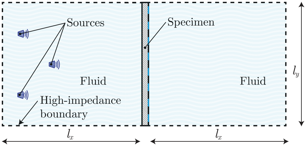
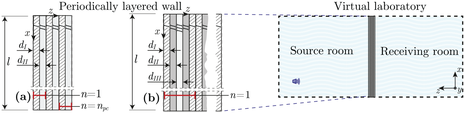
The schematic of the virtual laboratory is shown in Figure 3. As recommended in the DIN EN ISO 10140, the dimensions $l_x\sim \sim 5$ m and $l_y\sim \sim 4$ m of the rooms are sufficiently large. The sound velocity $c_0$ in the air is set to 341 $m\mathrm{/s}.$ A high impedance is assigned to the walls of the laboratory, equivalent to an absorption coefficient $\alpha \approx 95\%,$ see equation (5).

Figure 3.

Schematic of the virtual acoustic laboratory.

Sound sources described by equation (2) are used. The influences of the geometrical and material parameters like the size of the virtual laboratory, the absorption coefficient, the mounting of the specimen or the effect of flanking transmission could be quite high. For detailed studies we refer to Maluski and Gibbs, ⁶ Ackermann ¹¹ and Gibbs and Maluski ³⁵

The diffusivity of the sound field in a test laboratory is of major importance for the evaluation of the sound transmission of standard walls. In Papadopoulos,^13,14 the geometry of a virtual laboratory has been modified in order to increase the diffusivity. However, for the present investigation of periodic walls, the influence of the diffusivity of the sound field in the two virtual testing rooms is relatively small in comparison to the resonance and scattering effects within the periodic structure, especially at high frequencies. For this reason, we use rectangular testing rooms in our virtual laboratory and do not consider the diffusivity effect in detail.

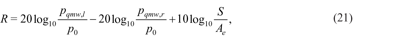
To calculate the transmission loss, referred to as the sound reduction index $R,$ equation (18) is solved numerically for the pressure distribution in the fluid domains and then $R$ is obtained by

$$R=20{\log }_{10}\frac{p_{qmw,l}}{p_0}-20{\log }_{10}\frac{p_{qmw,r}}{p_0}+10{\log }_{10}\frac{S}{A_e},$$

(21)

with the mean square root $p_{qmw}=\frac{p}{\sqrt{2}}$ for the source room (denoted by $l$ ) and the receiving room (denoted by $r$ ). The reference pressure is $p_0=2\times {10}^{-5}$ $\mathrm{W/m},$ and $S$ and $A_e$ are the area of the wall specimen and the equivalent absorption area. The equivalent absorption area is defined by

$$A_e=\sum _{i=1}^{i_{max}}{\alpha }_i{A}_i$$

(22)

with the surface areas of the source room $A_i$ and their respective absorption coefficients ${\alpha }_i.$ The lengths of the sides of the source room and the width of the specimen are used for a 2D calculation as an approximation with $i_{max}=3$ . We refer to Möser ³⁶ for more details.

Periodic wall structures

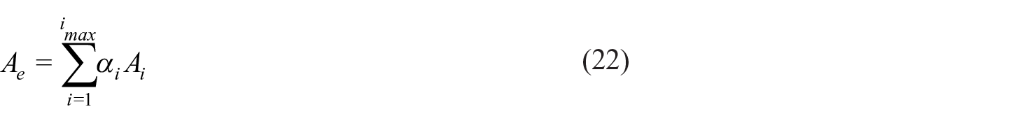
This work examines two kinds of periodically arranged wall structures. In the 1D periodic wall, the layers repeat periodically in the normal direction of the wall. In the 2D periodic structure, the wall consists of the so-called unit-cells which repeat periodically in the $z$ -direction and the $x$ -direction (see Figure 4). Since the length of the wall $l$ is usually far larger than the length of the unit-cell, the relevant number of the unit-cells in the normal direction of the wall is $n_{pc}.$ However, the length of the wall has also some influences in certain 1D cases.

Figure 4.

Schematic of a 2D periodically arranged wall.

The general behavior of the wave propagation in the periodic structures can be determined by an eigenvalue calculation of the domain formed by the unit-cell for different values of the wave vector $k.$ The wave vector is varied within the corners $\Gamma ,$ X and M, the so-called irreducible first Brillouin zone (IBZ),^37,38 as shown in the unit-cell in Figure 4. The following periodic Bloch boundary conditions are assigned on ${\Gamma }_{BF}:$

$${\mathit{u}}_z={\mathit{u}}_q{e}^{-ik\cdot \left({\mathit{r}}_z-{\mathit{r}}_q\right)},$$

(23)

where $z$ is the target boundary, $q$ is the source boundary and $r$ is the position vector. The implementation of the boundary conditions is described in detail in the work of Veres et al. ³⁹

It should be emphasized here that the Bloch boundary conditions are only applied to the unit-cell of an infinite periodic wall structure (but not the finite periodic wall structure in the fluid-structure interaction model) for the calculation of the dispersion diagrams (see the left figure in Figure 4). This technique is common to analyze the dispersion properties of an infinite periodic structure in a certain frequency range and optimize the geometry of the unit-cell with regard to a wide and low-frequency band-gap. It should also be noted, that for simplicity the IBZ in this work is restricted to the high symmetry points $\Gamma ,$ X and M (even though for some unit-cells considered in this paper additional high symmetry points exist) since only these points are relevant for the determination of the SRI by the proposed virtual acoustic laboratory.

Accuracy and efficiency of the virtual acoustic laboratory

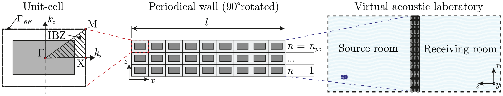
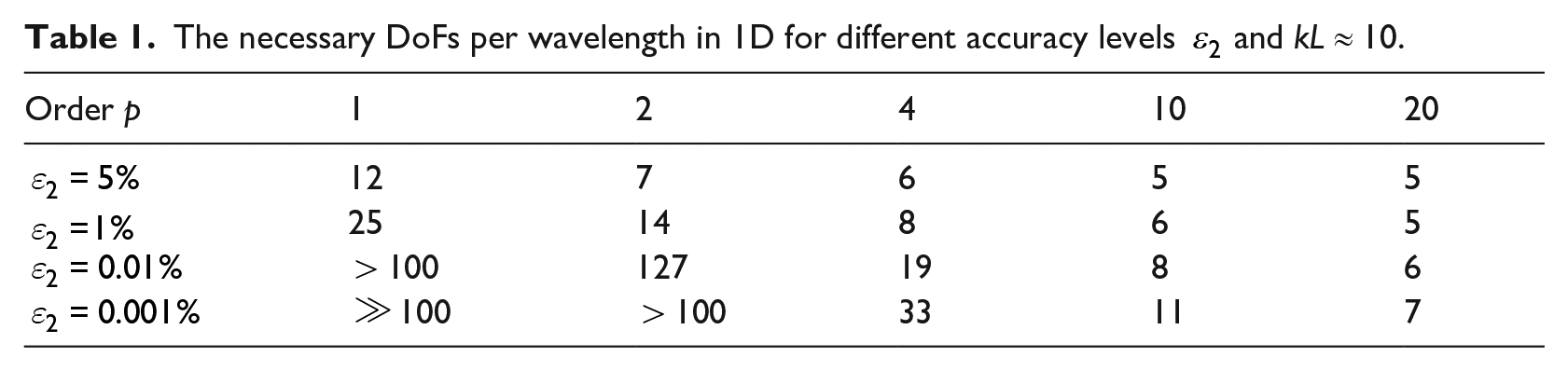
The SEM is very efficient, especially for problems that require a high accuracy. The spectral convergence leads to a significant reduction in the required degrees of freedom (DoFs) per wavelength. A comparison for a small wavenumber $k$ is given in Table 1, where the error is computed for a 1D Helmholtz problem with non-reflecting boundary conditions and sufficiently small length $L$ so that $kL$ is very low. The error is defined by

$${\epsilon }_2=100\frac{\sqrt{\sum _{n=1}^{N_{sp}}{\left(p_n^{SEM}-p_n^{ref}\right)}^2}}{\sqrt{\sum _{n=1}^{N_{sp}}{\left(p_n^{ref}\right)}^2}},$$

(24)

with the reference solution $p^{ref}$ (calculated with a very high accuracy by using a large number of DoFs per wavelength and a high order $p$ ) and the SEM solution $p^{SEM}.$ $N_{sp}$ is the number of sample points used to calculate the error. As an example, for ${\epsilon }_2=0.01\%$ and $k=1{\mathrm{m}}^{-1},$ approximately 250 DoFs are needed in a 1D problem with $L=2$ m and $15.6\cdot {10}^6$ DoFs are needed in a 3D problem with $L^3=8{\mathrm{m}}^3$ if we choose $p=2$ . For $p=10,$ only 16 DoFs are needed in the 1D problem and $4100$ DoFs are needed in the 3D problem. Obviously, for a high accuracy or a low error ${\epsilon }_2,$ it is very advantageous to use a high order $p,$ especially for 2D and 3D problems.

Table 1.

The necessary DoFs per wavelength in 1D for different accuracy levels ${\epsilon }_2$ and kL ≈ 10.

Order p	1	2	4	10	20
${\epsilon }_2=5\%$	12	7	6	5	5
${\epsilon }_2=1\%$	25	14	8	6	5
${\epsilon }_2=0.01\%$	> 100	127	19	8	6
${\epsilon }_2=0.001\%$	≫ 100	> 100	33	11	7

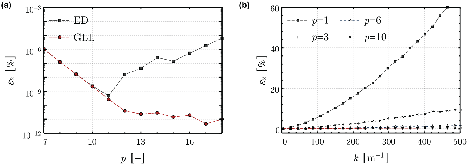
It should be noted, that the number of the necessary DoFs is usually higher due to the numerical dispersion at higher frequencies. ⁴⁰ Thus, Table 1 should only be regarded as an approximate guideline for selecting the necessary discretization level for the intended accuracy of the solution. Numerical dispersion is basically the increase of the error of the numerical solution at higher wavenumbers. It is visible in Figure 5(b), that a choice of a high order $p$ lowers the error for high wave numbers $k$ and thus limits the negative effect of the numerical dispersion.

Figure 5.

Error for the 1D Helmholtz equation $\Delta p+k^{2}p=0$ with Dirichlet boundary conditions and its variation with (a): the order of the shape functions $p$ and (b): the wave number $k.$

As mentioned previously, the condition number of the linear system of algebraic equations is lower if we use the GLL shape functions instead of the ED shape functions. This results in a better numerical behavior for a high order $p$ of the shape functions (see Figure 5(a)) and also for inherently ill-conditioned problems. These include problems in the close proximity of eigenfrequencies, crucial material parameters such as Poisson’s ratio $\nu \sim \sim 0.5,$ or a strongly distorted mesh. The general correlations shown in Figure 5 for a simple 1D Helmholtz problem also hold for complex FSI problems.

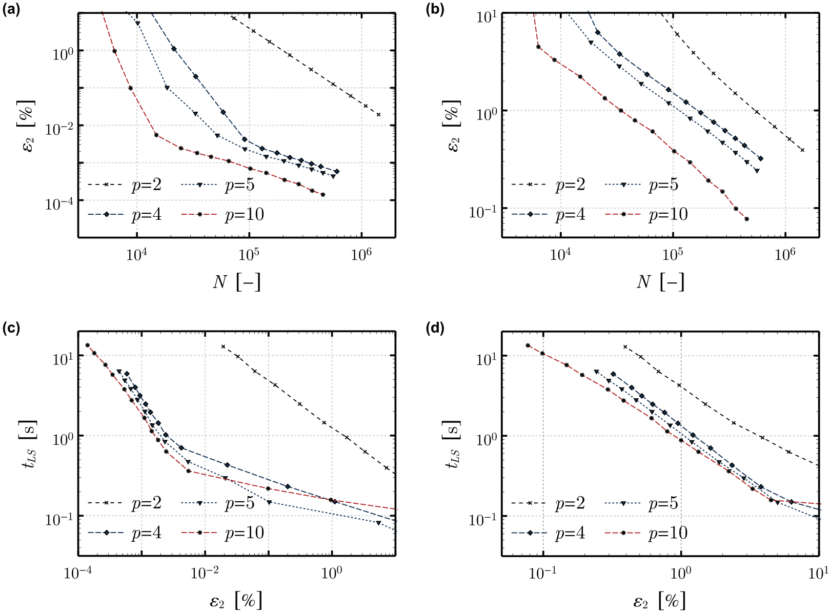
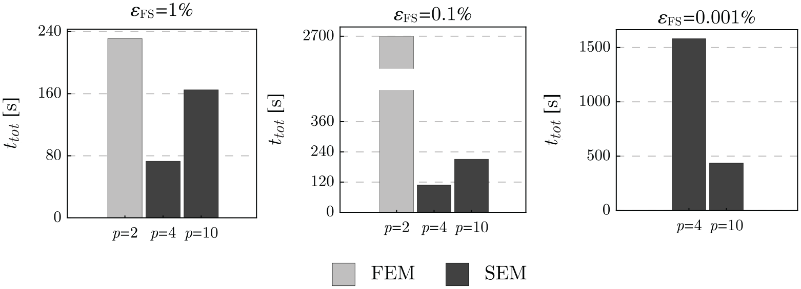
While the use of a high order $p$ decreases the necessary number of DoFs, the required time for solving the resulting linear system $t_{LS}$ does not necessarily reduce. This is because that the sparsity (the relative number of zero elements) of the coefficient matrix decreases and the solution of the linear system of algebraic equations becomes less efficient. This is shown for the virtual laboratory in Figure 6 for solving equation (18) at $f=3500$ Hz. While the use of $p=10$ is efficient for a high accuracy, for a low accuracy the solution of the linear system is less time-intensive if we use a lower order $p.$ Figure 6(c) and (d) show the time required for solving the linear system of $N$ algebraic equations for only one frequency, and Figure 7 shows the time needed for the calculation of the SRI for the entire frequency range by the developed algorithm. The frequency range includes 16 1/3-octaves from 100 Hz until 3150 Hz and a total number of 336 discrete frequencies. In general, while for a low accuracy a lower order $p$ is used, the calculation is far more efficient for a higher accuracy, if a high order is used. The calculation time in this work was measured on a standard desktop computer (a calculation for $p$ =2 and ${\epsilon }_{FS}=0.001\%$ was not possible due to insufficient random-access memory of the computer). Usually, the efficiency of the SEM is limited due to the increased calculation time of the element matrices for higher orders. An increased efficiency for higher orders is achieved in this work by precalculating the system matrices for the fluid domains ${\mathit{K}}_{F_{1,2}}$ and ${\mathit{M}}_{F_{1,2}},$ storing them on the computer and using them for different wall structures. For this reason, we exclude the time needed for the calculation of the element matrices for the fluid domains in Figure 7. To define an a priori accuracy level for the calculation we used the number of nodes per wavelength according to the desired ${\epsilon }_{FS}$ in Table 1. In order to indicate that this a priori accuracy level is not the real error (due to the more complex geometry, the FSI interaction, the numerical dispersion and the influence of eigenfrequencies), we call this the accuracy level ${\epsilon }_{FS},$ which simply indicates the number of DoFs we used per wavelength in the calculation according to Table 1. The calculation time $t_{tot}$ results mainly from the assembly and solution of the linear system for each frequency. The assembly process is more efficient, if the Lobatto quadrature is used for the numerical integration of the element mass matrices since ${\mathit{M}}_{F_{1,2}}$ and ${\mathit{M}}_S$ are then diagonal and the number of operations for assembly of the linear system in equation (18) decreases for each frequency. This leads to an efficiency increase of roughly 10–20%. It should be mentioned here that the diagonal element mass matrices also allow for the use of an explicit time integration method to solve the corresponding FSI problems in the time-domain. ⁴¹

Figure 6.

The numerical error ${\epsilon }_2$ for different discretization levels for (a) the source room and (b) the receiving room, where $N$ is the number of DoFs. The required time for solving the linear system of algebraic equations $t_{LS}$ for $f=3500$ Hz and (c) the source room and (d) the receiving room.

Figure 7.

Comparison of the required time $t_{tot}$ to calculate the SRI curve for different accuracy levels.

The last question to be discussed in this section is the necessary number of DoFs per wavelength. For conventional wall constructions, a relatively low accuracy is usually sufficient for the virtual laboratory if the main goal is the prediction of the SRI curve or the comparison with measurements in a real laboratory. Figure 8(a) shows the 1/3-octave averaged deviations for a concrete wall from the reference solution, which is calculated with a very high accuracy by using a large number of DoFs per wavelength and a high order $p.$ The results of the reference solution are also compared with that obtained by commercially available FEM-Software (COMSOL Multiphysics Version 5.3) using a large number of DoFs, and no significant deviations are found. The averaging of the SRI for all frequencies of a 1/3-octave reduces the influence of the eigenfrequencies, but this requires a large number of frequencies to be considered. For the determination of the 1/3-octave SRI curve, we found that at least 10–20 frequencies should be considered for every 1/3-octave.

Figure 8.

(a): Deviations ∆ $R$ of the $1/3$ -octave averaged SRI from the reference solution for a monolithic wall and (b): Deviations of the SRI for a periodically layered wall.

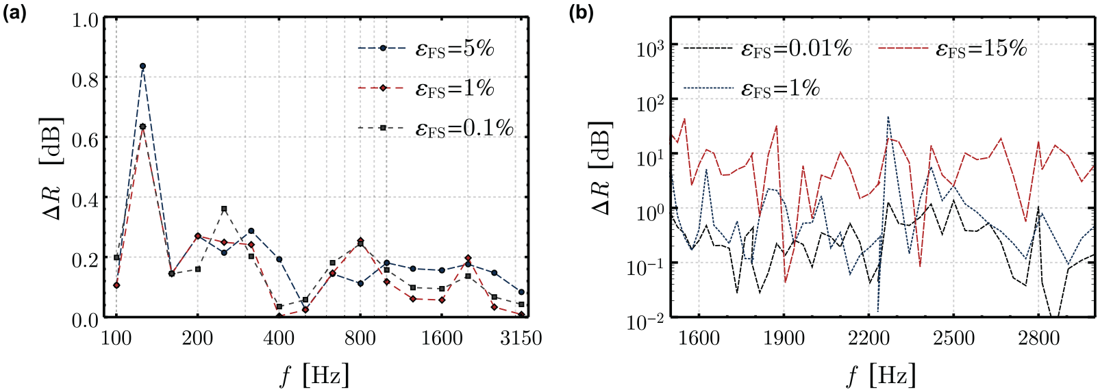
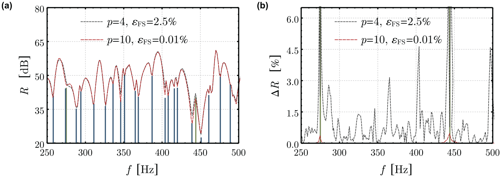
For a detailed analysis of the frequency range, a higher accuracy should be chosen, since the deviations increase in the proximity of the eigenfrequencies, as shown in Figure 9 for a concrete wall. The necessary accuracy should also be increased for the study of periodic structures. In Figure 8(b) the deviations for a 1D periodic wall and different accuracy levels are shown. In the band-gap the deviations are up to almost 100 dB. After averaging over a 1/3-octave interval, this still amounts to remarkable deviations higher than 10 dB.

Figure 9.

(a): The SRI R and (b): its deviation ∆ $R$ from the reference solution with very high accuracy in the proximity of the eigenfrequencies for different discretization orders $p.$ The dark green lines mark the wall eigenfrequencies and the blue lines mark the room eigenfrequencies.

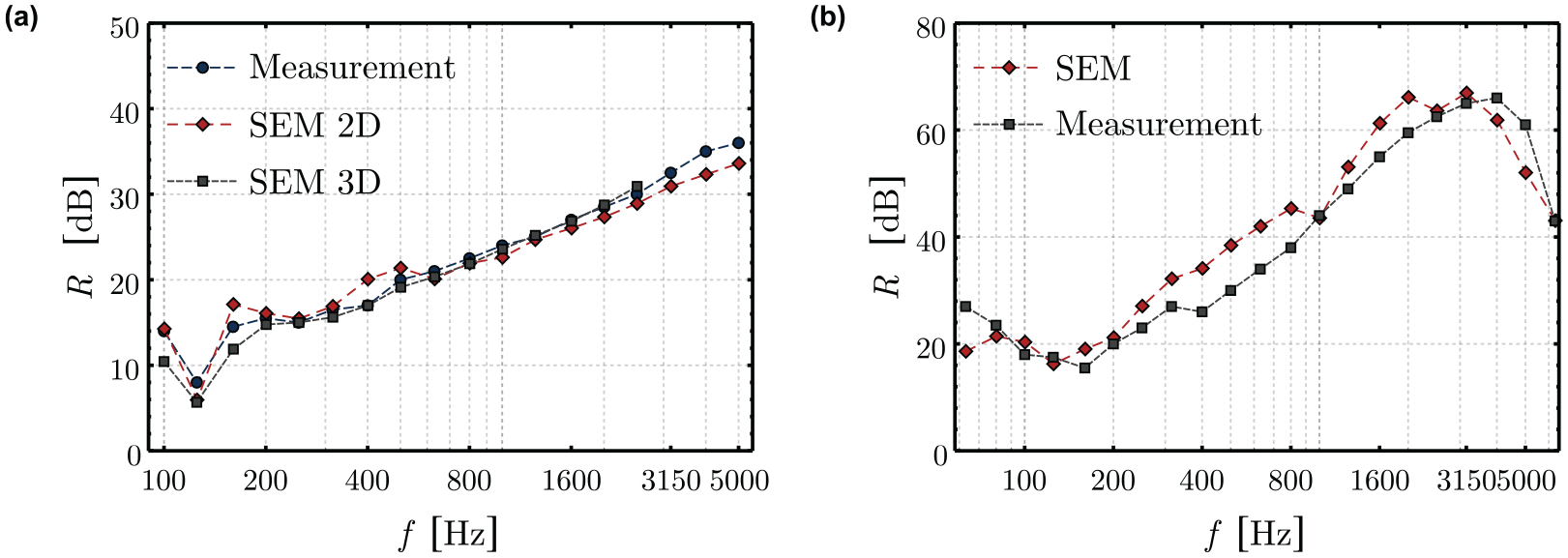
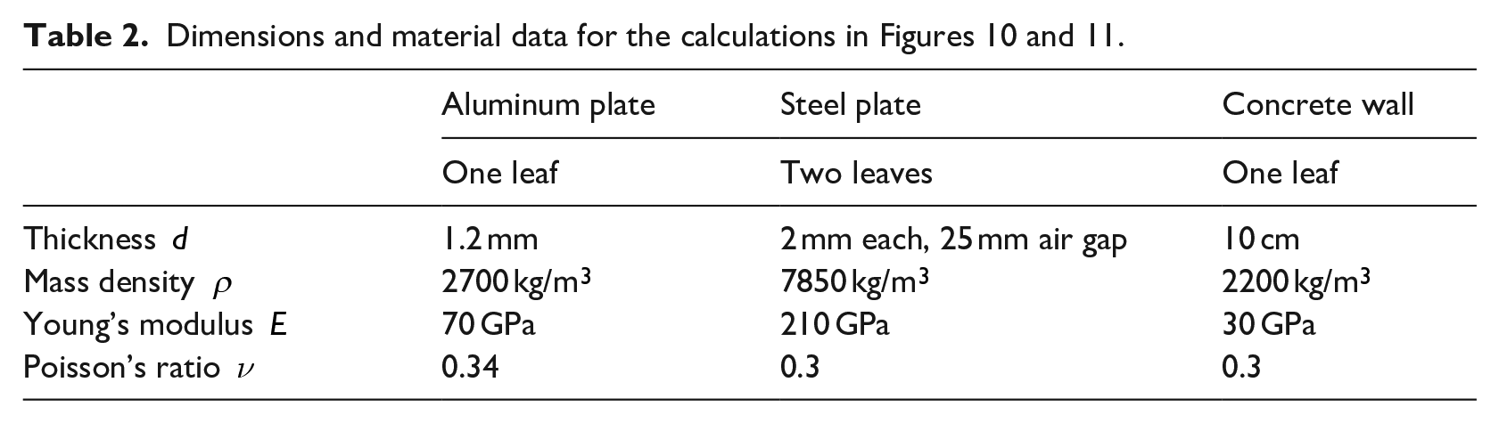
In general, the results agree well with the experimental data as shown in Figure 10, despite some deviations which are possibly due to the limited knowledge about the exact properties of the wall specimen and measurement laboratory. The dimensions and material data are given in Table 2. The comparison in Figure 10(a) also demonstrates that a 2D calculation is sufficient if the structure fulfills the plane strain condition. One of the advantages of the virtual laboratory is its flexibility. Analytical solutions for complex problems usually require a high level of simplifications. For the approach in this work, complex structure or material models can be directly simulated and do not require many simplifications. Another advantage is the amount of information provided by this approach. Not only the SRI curve can be obtained, but also the details about the pressure field in the fluid and the displacement field of the wall specimen.

Figure 10.

Comparison between the calculated SRI by the FSI model (SEM) and the measured SRI for a thin aluminum plate (a) and a double-leafed steel plate (b). The measurement data are taken from Villot et al. ⁴² for the aluminum plate and from Hongisto et al. ⁴³ for the double-leafed steel plate.

Table 2.

Dimensions and material data for the calculations in Figures 10 and 11.

	Aluminum plate	Steel plate	Concrete wall
	One leaf	Two leaves	One leaf
Thickness $d$	1.2 mm	2 mm each, 25 mm air gap	10 cm
Mass density $\rho$	2700 ${\mathrm{kg}/\mathrm{m}}^3$	7850 ${\mathrm{kg}/\mathrm{m}}^3$	2200 ${\mathrm{kg}/\mathrm{m}}^3$
Young’s modulus $E$	70 GPa	210 GPa	30 GPa
Poisson’s ratio $\nu$	0.34	0.3	0.3

Figure 11.

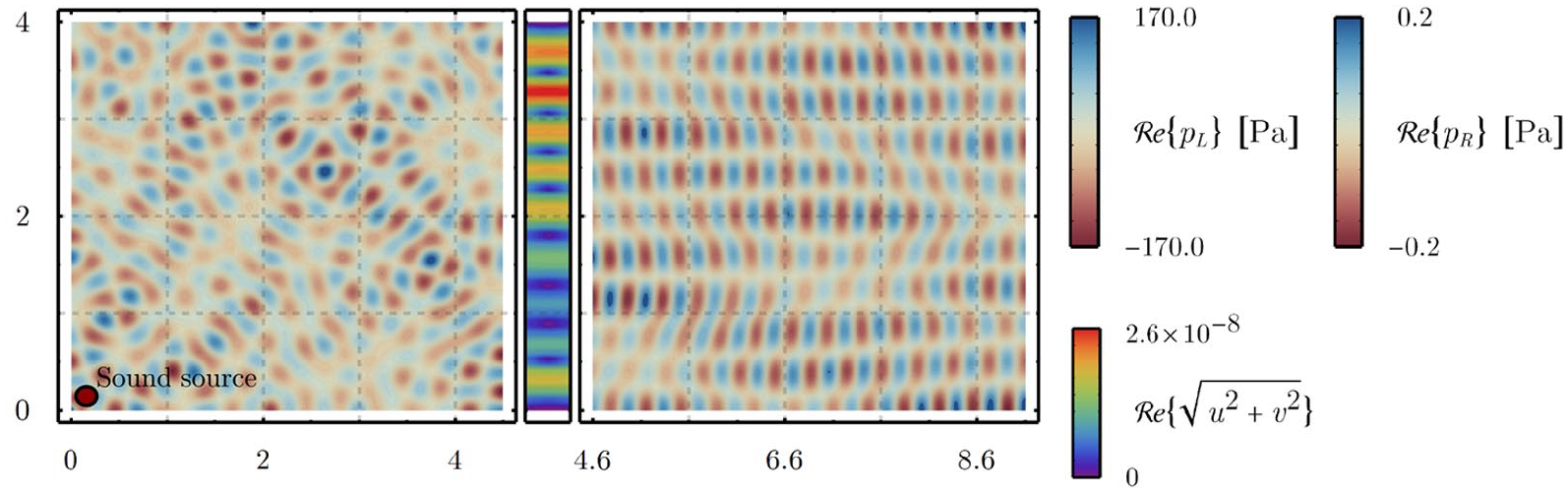
Real part of the pressure field and the displacement field of a concrete wall with a thickness of 10 cm at $f=1000$ Hz. Note: The high values for the pressure field are a result of the power of the sound source, which is normalized to unity. This has no effect on the SRI.

An example for a concrete wall of 10 cm thickness is shown in Figure 11 for $f=1000$ Hz. This is especially useful for the detailed study of periodically arranged wall structures and their behavior in different frequency ranges.

Numerical examples for periodic walls

1D periodic walls

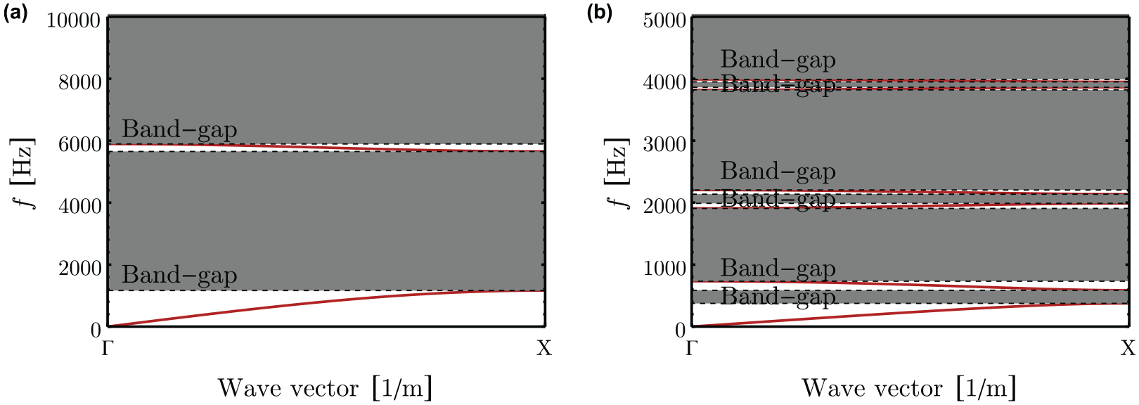
For a 1D periodically layered wall, we examine two different examples (see Figure 12). The unit-cell $1_{1D}$ consists of two layers where two different materials are used for the periodically layered wall, denoted by $I$ and $II$ . The unit-cell $2_{1D}$ consists of five layers and three different materials denoted by $I,$ $II$ and $III.$ Figure 13 shows the dispersion diagrams for both unit-cells. The frequency ranges in which the wave propagation is prohibited, the so-called band-gaps, are marked by gray areas. The dispersion diagrams show a theoretical behavior for an infinite number of unit-cells. Since we are interested in the behavior of a finite wall structure and the influences of various parameters on the SRI, we conduct further examinations via the virtual laboratory. The number of the unit-cells is $n_{pc}$ and the $z$ -direction is normal to the wall surface (the direction of the sound transmission through the wall). Since the length $l$ of the wall may influence the frequency response significantly in certain cases, we examine the efficiency of the periodic wall structures directly with respect to the SRI curves. For the figures depicting a frequency response or displacement field in this work, the denotation of the unit-cell refers to a wall consisting of the respective unit-cell and the calculation according to the methodology described previously.

Figure 12.

Schematic of the periodically layered walls. (a): The 1D unit-cell $1_{1D}$ consists of two layers and (b): the 1D unit-cell $2_{1D}$ consists of five layers.

Figure 13.

Dispersion diagrams for (a) the unit-cell $1_{1D}$ and (b) the unit-cell $2_{1D}.$ The gray areas mark band-gaps.

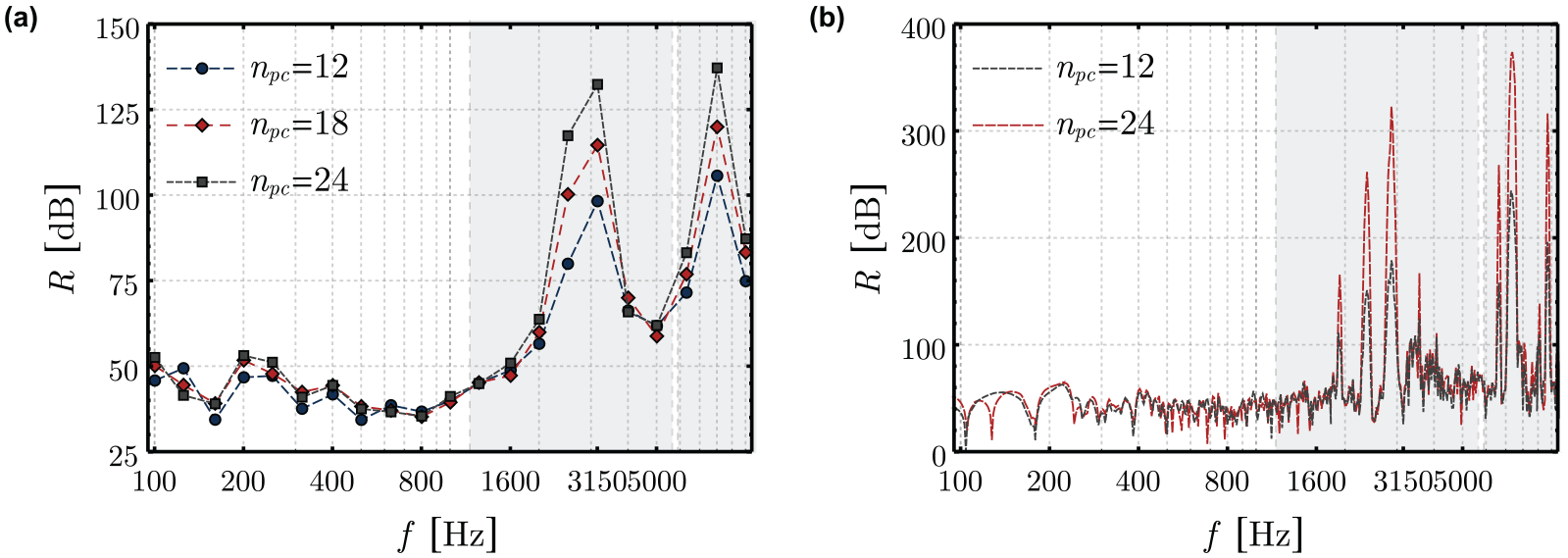
We begin with the examination of the unit-cell $1_{1D}.$ A cork-like material with the following material parameters is used for layer $I:$ mass density ${\rho }_I=250\mathrm{kg}/{\mathrm{m}}^3,$ Young’s modulus $E_I=0.02$ GPa, and Poisson’s ratio ${\nu }_I=0.05$ . Concrete is used for layer $II.$ For the unit-cell $1_{1D}$ and all other unit-cells in this section we use the following material properties for concrete: ${\rho }_{II}=2300{\mathrm{kg}/\mathrm{m}}^3$ , $E_{II}=25$ GPa and ${\nu }_{II}=0.2$ . Since the focus of this examination is to investigate the attenuation of the periodically layered wall structure due to resonance and interference effects, we do not use any material damping here. The thicknesses of the layers are set to $d_I=0.025$ m and $d_{II}=0.025$ m. Figure 14(a) shows the SRI curves for different numbers of the unit-cells $n_{pc}.$ For clarity, the frequency responses are averaged over each $1/3$ -octave. From the figure, it can be concluded, that the SRI in the band-gaps increases with the number of unit-cells by approximately 2.5 dB per unit-cell. On the other hand, in the frequency ranges outside of the band-gaps, increasing the number of the unit-cells leads to an increase of the mass of the wall structure which is the reason for some small gains of the SRI. Note the small length $l$ , the increase of the SRI within the band-gaps is less pronounced for larger values of $l$ (see the Figure 15(a)). Figure 14(b) shows the detailed SRI (frequency response). The maximum value of the SRI is increasing with increasing value of $n_{pc}.$ The SRI is exceeding a value of 120 dB for a sufficient number of unit-cells $n_{pc}$ , especially at certain frequencies in Figure 14(b). This effect will be far more pronounced for more complex unit-cells, which will be shown in the following examples and discussions. Since the virtual laboratory considers the mostly important physical effects, which would influence the behavior of the specimen in a real test laboratory, the obtained SRI results should be capable of representing the realistic performance of the investigated periodic wall structures. Although no experimental verifications in a real test laboratory for the examined periodic wall structures are conducted in this work, experimental investigations of similar problems show indeed the extraordinary wave insulation properties of the periodic structures, for example Vasseur et al.^44,45 or Sigalas et al. ⁴⁶ In general, the width of the “band-gaps” (the band-gaps, which occur in a practical application and differ from the theoretical obtained band-gaps in Figure 13) are very narrow. Furthermore, various resonance effects of the virtual laboratory can also decrease the SRI within the band-gaps obtained by calculation of the dispersion diagram.

Figure 14.

(a): $1/3$ -octave averaged SRI and (b): SRI (frequency response) for different values of $n_{pc}$ for the periodic wall consisting of unit-cell $1_{1D}$ and $l=1$ m. The gray areas mark the band-gaps obtained from the calculation of the dispersion diagram in Figure 13(a).

Figure 15.

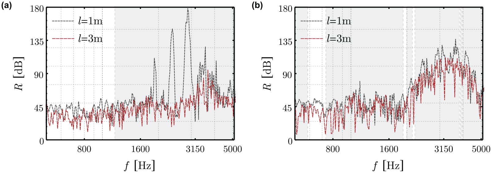
Frequency response for (a): the periodic wall consisting of unit-cell $1_{1D}$ with two layers and (b): the periodic wall consisting of unit-cell $2_{1D}$ with five layers for different values of the wall length $l$ respectively. The gray areas mark the band-gaps obtained from the calculation of the dispersion diagrams in Figure 13(a) and (b).

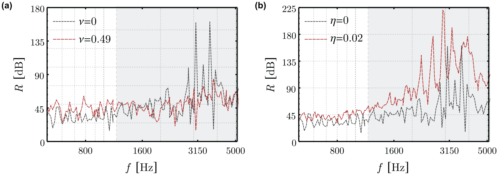
A comparison for different values of $l$ is shown in Figure 15(a). The reason for this behavior in Figure 15(a) probably due to the influence of the transverse deformation and the reflections on the clamped boundaries of the wall structure. The 1D periodic structure supports indeed longitudinal waves primarily in one direction, but the generation of shear waves is still possible through Poisson’s ratio. Due to the wave reflections on the boundaries, these shear waves, in turn, generate longitudinal waves which decrease the efficiency of the periodic wall structure. This can be demonstrated by the influence of Poisson’s ratio $\nu ={\nu }_I={\nu }_{II}$ as shown in Figure 16(a). For small values of $\nu$ , the efficiency of the periodic wall structure increases. The efficiency is also increased by including the material damping, as shown in Figure 16(b).

Figure 16.

Effects of (a): Poisson’s ratio $\nu$ and (b): the loss factor $\eta$ for the periodic wall consisting of unit-cell $1_{1D}$ for $n_{pc}=24$ . The gray area marks the band-gap obtained from the calculation of the dispersion diagram in Figure 13(a).

In summary, the performance of the unit-cell $1_{1D}$ is rather poor. The necessary high value of $n_{pc}$ increases the thickness of the wall to impractical values and realistic applications would also require larger values of $l$ . However, the setup of the unit-cell $2_{1D}$ is far more promising. By embedding an additional layer of steel, the number of necessary layers and the negative effects of the length of the wall $l$ can be significantly reduced. The corresponding setup is shown in Figure 12. The thickness of the steel layer is set to $d_{III}=0.005$ m and the thickness of the layers $I$ and $II$ is set to $d_I=d_{II}=0.025$ m. Concrete is used for layer $I$ and a rubber-like material is used for layer $II.$ The parameters used for the rubber-like material are ${\rho }_{II}=1100{\mathrm{kg}/\mathrm{m}}^3$ , $E_{II}=0.01$ GPa, ${\nu }_{II}=0.45$ and for steel we use ${\rho }_{III}=7850{\mathrm{kg}/\mathrm{m}}^3$ , $E_{III}=210$ GPa, ${\nu }_{III}=0.3$ .

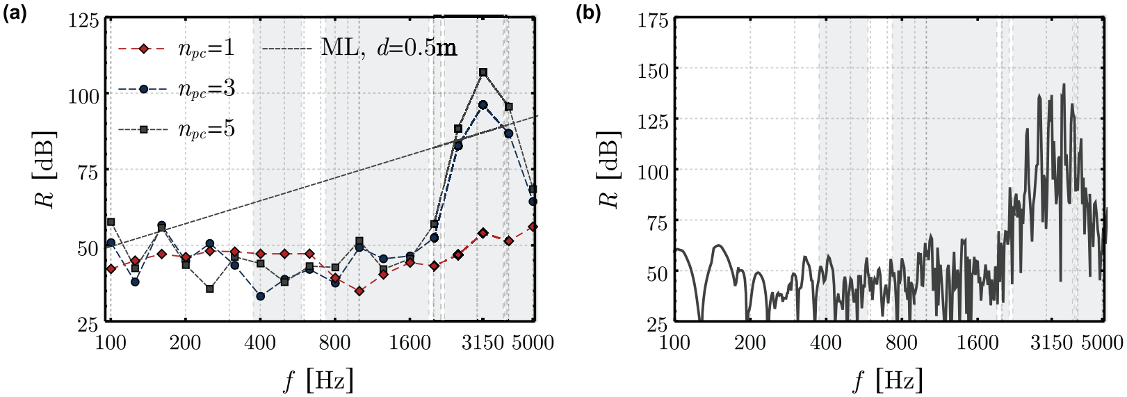
The resulting curves of the SRI are shown in Figure 17(a) for different numbers of the unit-cells consisting of five layers. The gain for each additional unit-cell is much higher and reaches approximately 10 dB per unit-cell in the band-gap. The increase of the SRI in the frequency range outside of the band-gap is only a result of the additional mass and stiffness of the structure. A monolithic concrete wall of thickness $d=0.5$ m is also included in the figure to illustrate the extreme values of the SRI in the band-gap, which can only be achieved by a periodically arranged wall structure. Doubling the thickness of the periodically layered wall $(n_{pc}=5)$ would increase the SRI by about 50 dB while doubling the thickness of the concrete wall would only increase the SRI by about 8 dB. The detailed SRI (frequency response) is depicted in Figure 17(b). While the SRI in the frequency range of the band-gap is in general increased by the periodic arrangement, other resonance phenomena can superpose the interference effects and lead to some drops. However, the band-gap for the unit-cell $2_{1D}$ is clearly more distinct than the band-gap of the unit-cell $1_{1D}$ (compare the peaks and drops of Figures 14(b) and 17(b)). Since the resonance effects due to the steel layer are presumably the main reason for the efficiency of the unit-cell $2_{1D},$ there is also very little negative influence of the length of the wall $l,$ as shown in Figure 15(b). On the other hand, the result for the unit-cell $1_{1D}$ is believed to rely mainly on interference effects.

Figure 17.

(a): $1/3$ -octave averaged SRI for different values of $n_{pc}$ for the periodic wall consisting of the unit-cell $2_{1D}.$ ML denotes the SRI for a monolithic concrete wall of thickness $d=0.5$ m calculated by the mass law. ⁴⁷ (b): SRI (frequency response) for $n_{pc}=5$ . The gray areas mark band-gaps obtained from the calculation of the dispersion diagram in Figure 13(b).

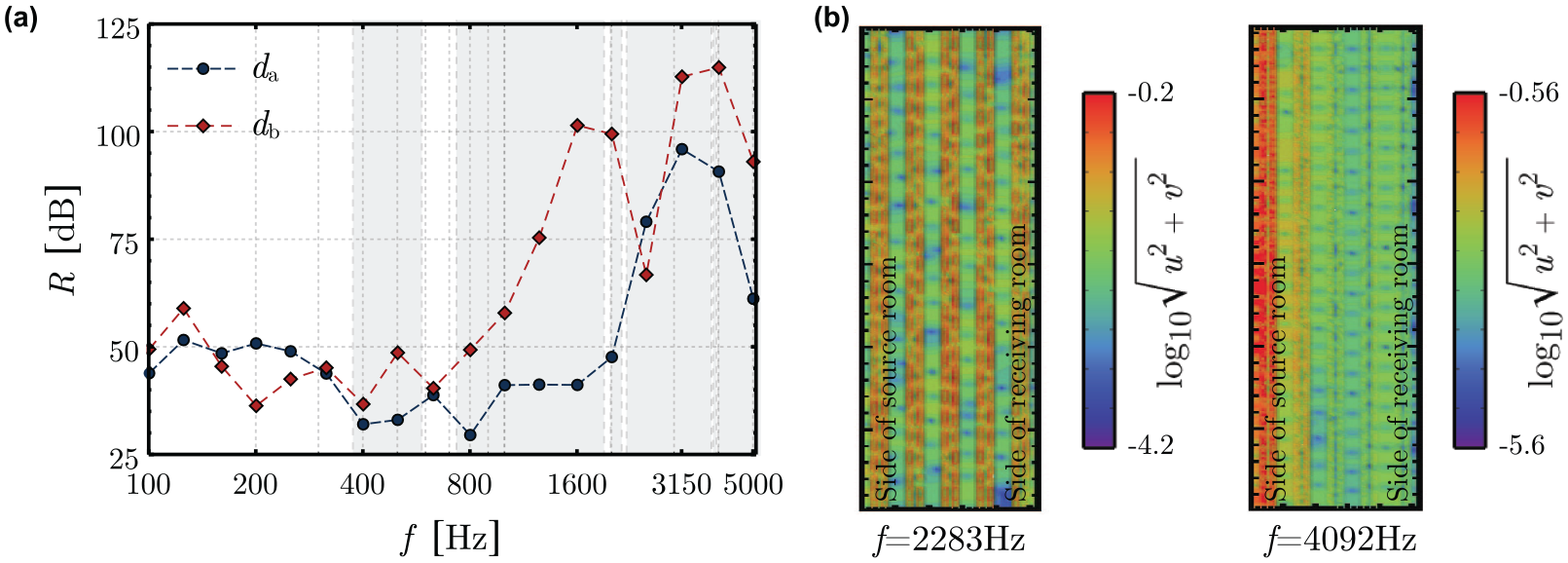
The position and width of the band-gaps as well as the effectiveness of the periodical arrangement are determined by the material properties of the constituting layers and their thicknesses. To demonstrate the thickness-dependence, the thicknesses of the layers are varied in Figure 18(a) for the unit-cell $2_{1D}.$ By doubling the thicknesses of the layers, the frequency range of the band-gap is reduced by $50\%$ . This also applies for the 2D unit-cells we will discuss in the following subsection. Figure 18(b) shows the logarithmic displacement field for a layered wall (unit-cell $2_{1D})$ at a frequency outside and inside of the band-gaps. It can be observed, that the wave propagation is severely restricted inside of the band-gap.

Figure 18.

(a): $1/3$ -octave averaged SRI for different thicknesses of the unit-cell $2_{1D}:$ $d_I=d_{II}=0.025$ m, $d_{III}=0.005$ m for $d_a$ and $d_I=d_{II}=0.05$ m, $d_{III}=0.01$ m for $d_b$ . The gray areas mark band-gaps obtained from the calculation of the dispersion diagram in Figure 13(b) for the dimensions $d_a$ . (b): Logarithmic displacement field for the unit-cell $2_{1D}$ at $f=2283$ Hz (outside of the band-gap) and $f=4092$ Hz (within the band-gap).

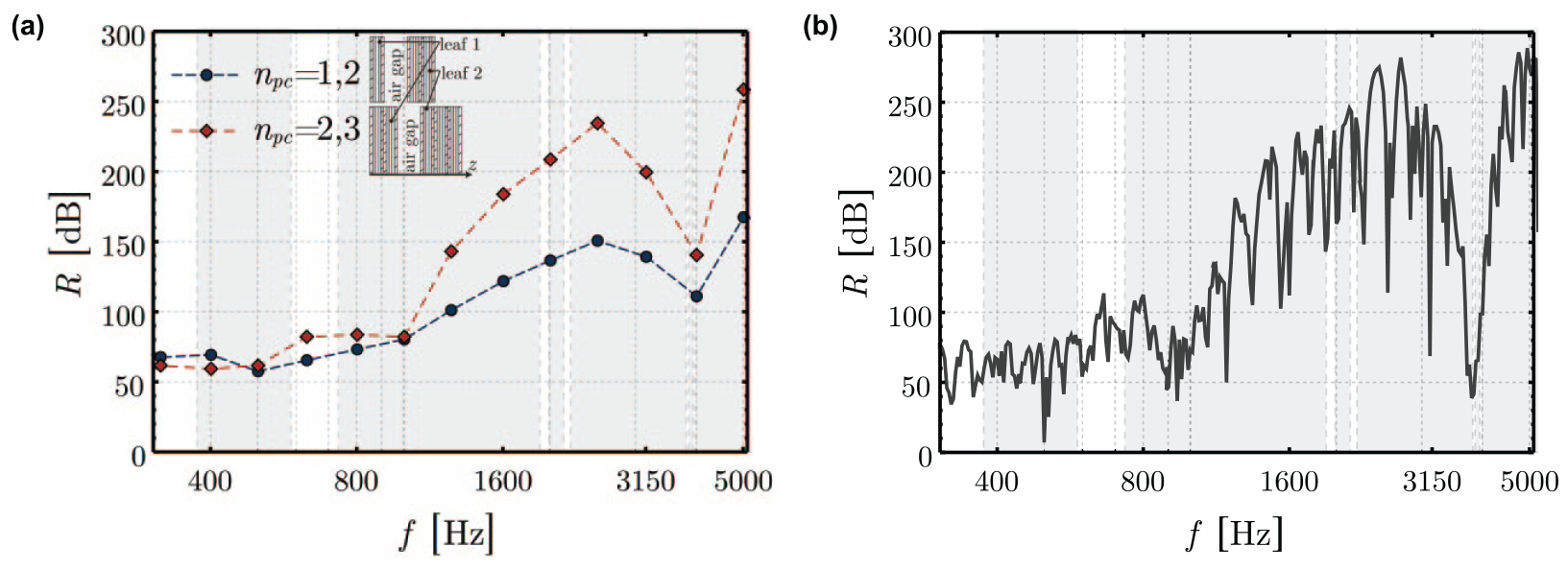
As the last example for the 1D periodically layered wall, we examine the efficiency of a double-leafed wall consisting of the unit-cells $2_{1D}.$ Both leaves are separated by an air gap, therefore combining the resonance effects of the double-leafed setup and the periodicity of the leaves themselves. The length of the wall is $l=2$ m and the two leaves are not connected. As expected, the performance within the band-gap is very good, even for a small thickness of the wall (see Figure 19 in which $n_{pc}=\alpha ,\beta$ indicates the number of $\alpha$ unit-cells $2_{1D}$ in the $z$ -direction for the first leaf and the number of $\beta$ unit-cells $2_{1D}$ in the $z$ -direction for the second leaf). However, using linking elements to connect both leaves in the assemblage would reduce the efficiency. Since the focus of this work lies on the examination of the periodic wall structures, possible connectors between the adjacent leaves are not taken into account. However, connected leaves could be numerically simulated by simply linking the respective DoFs at the positions of the connectors or using more sophisticated methods, as described for example in Poblet-Puig et al. ¹²

Figure 19.

(a): $1/3$ -octave averaged SRI for different values of $n_{pc}$ for a double-leafed periodically layered wall consisting of the unit-cells $2_{1D}$ with a $0.1$ m air gap between the leaves. (b): SRI for $n_{pc}=2,3$ . The gray areas mark band-gaps obtained from the calculation of the dispersion diagram in Figure 13(b).

2D periodic walls

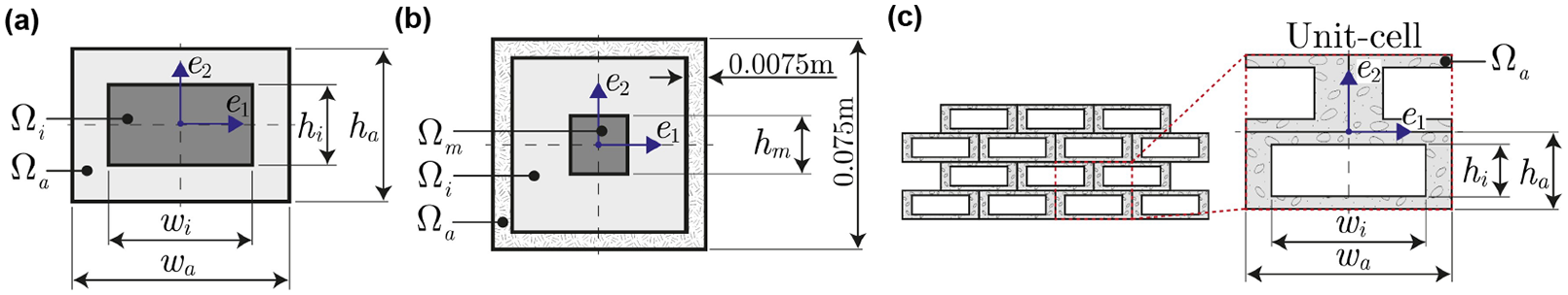
Figure 20 shows three different examples for a 2D unit-cell. The unit-cells are repeated along the vectors $e_1$ and $e_2$ to create the periodically arranged wall (see also Figure 4). The length of the wall $l$ is set to $\approx 2.5$ m for all 2D examples and no material damping is used in order to solely examine the effects of the periodical arrangement.

Figure 20.

Schematic of the three examined 2D unit-cells (a) $1_{2D}$ , (b) $2_{2D}$ and (c) $3_{2D}$ .

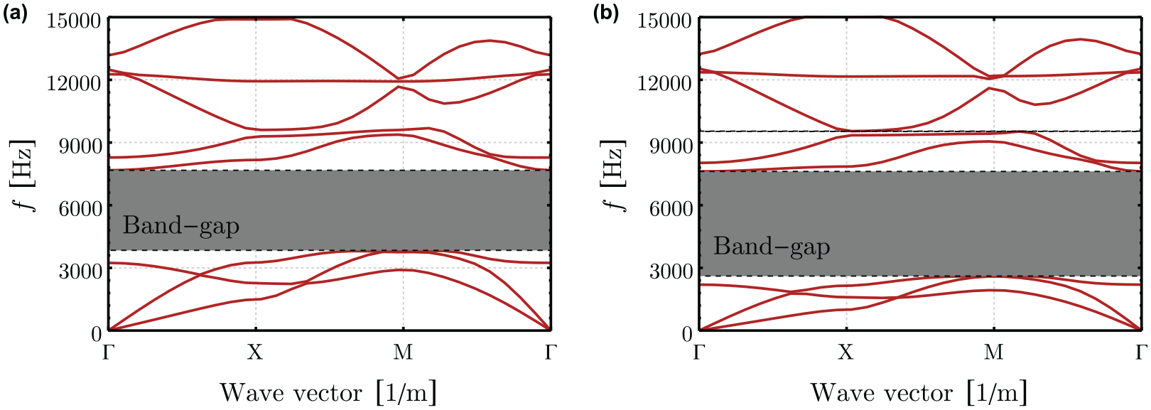
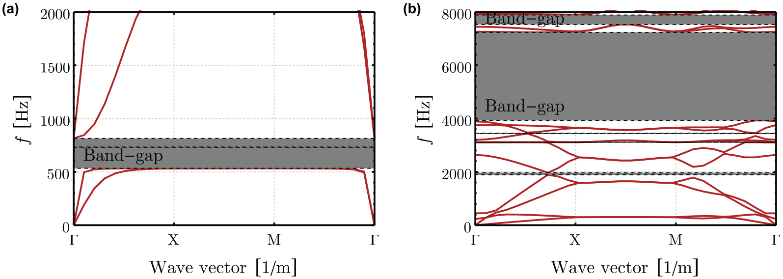
For the unit-cell $1_{2D}$ we use polyethylene ( $\rho =950\mathrm{kg}/{\mathrm{m}}^3$ , $E=1.040$ GPa, $\nu =0.46$ ) for the matrix $X_a$ and either steel or tungsten (the material properties of tungsten are: $\rho =19100\mathrm{kg}/{\mathrm{m}}^3$ , $E=410$ GPa, $\nu =0.28$ ) for the core $X_i$ . Since the 2D periodic wall structure does not allow wave propagation in both $x$ - and $z$ -directions within the band-gap, there is little influence of the transverse deformation. Therefore neither Poisson’s ratio nor the length of the wall $l$ has much impact on the efficiency of the 2D periodic wall structure. The examination of the dynamical behavior of the periodic wall structure can be simplified by calculation of the dispersion diagram as elucidated before. This allows us to efficiently optimize the geometry of the unit-cell in order to achieve a wide band-gap and also a preferable low-frequency band-gap, without increasing the thickness of the periodic wall to impractical values. The dispersion diagrams for a steel core and a tungsten core of the unit-cell $1_{2D}$ are shown in Figure 21. The dimensions of the unit-cell and the frequency range of the Bragg band-gap are inversely related according to the Bragg diffraction law. ⁴⁸ The midgap frequency $f_B$ is in the order of

$$f_b\approx \frac{c}{2a},$$

(25)

where $c$ is the velocity of the wave in the medium and $a$ is the lattice constant. For a more detailed description of the formation of Bragg band-gaps we refer to Kaina et al. ⁴⁹ and Khelif and Adibi. ⁵⁰

Figure 21.

Dispersion diagrams for the unit-cell $1_{2D}$ with $w_a=0.125$ m, $h_a=0.075$ m, $w_i=0.0875$ m, $h_i=0.0375$ m and (a) steel core, (b) tungsten core. The gray areas mark the band-gaps.

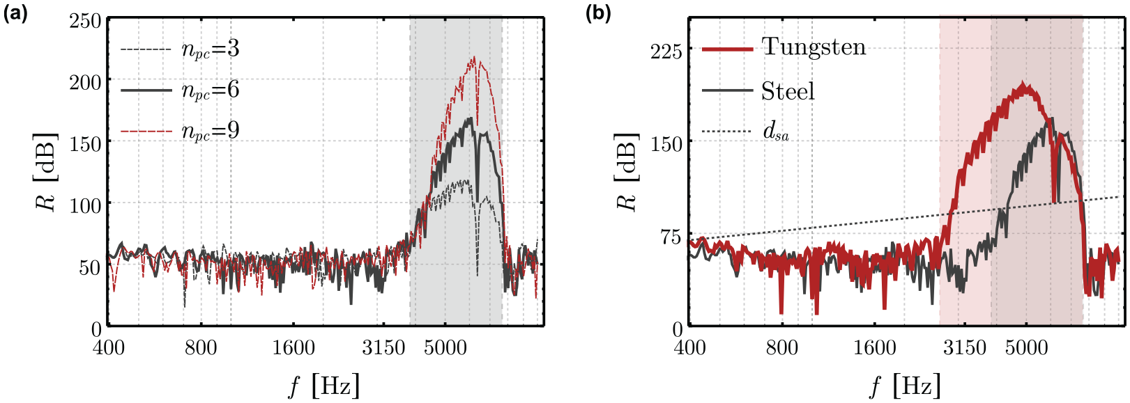
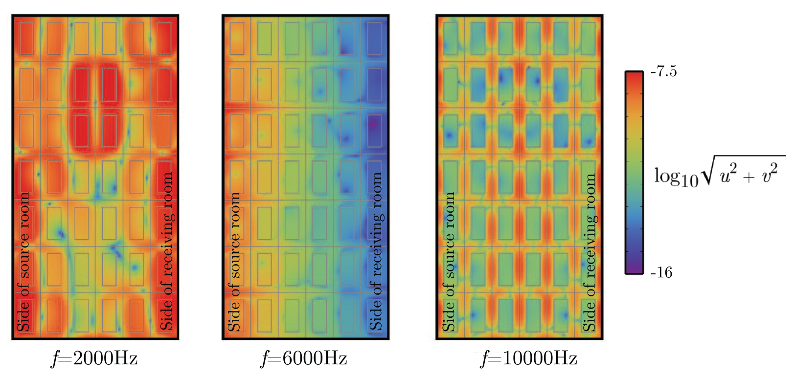
In general, the dispersion diagrams represent the wave propagation behavior within an infinite periodic structure. As also shown for the 1D examples, the actual attenuation can vastly differ in a finite structure, due to wave reflections on the boundaries and other resonance phenomena. Therefore we examine the performance of the more realistic finite periodic wall structure in the virtual laboratory for the 2D examples as well. Figure 22(a) shows the SRI (frequency response) for different numbers of the unit-cells in the $z$ -direction. The sound insulation increases by $\approx 20$ dB per unit-cell. A suitable way to improve the efficiency of the periodic wall structure is to use another material for the core or the matrix. In general, the mass density and the stiffness of the materials used should differ as much as possible. In Figure 22(b) tungsten with a higher stiffness and mass density is used for the core, and thus the width of the band-gap is increased and also its mid-frequency is lower. To show the significantly superior sound insulation capabilities of the periodic wall structure within the band-gap, the SRI for a monolithic steel wall with the same thickness is also included, which is denoted by $d_{sa}$ in Figure 22(b). Figure 23 shows the logarithmic total displacement fields for three different frequencies and $n_{pc}$ = 6.

Figure 22.

SRI curves for the wall consisting of the unit-cells $1_{2D}$ and (a): steel core with three different numbers of the unit-cells in the normal direction of the wall and (b): different materials for the core with $n_{pc}=6$ . The red and gray areas mark the band-gaps from the dispersion diagrams in Figure 21 steel core).

Figure 23.

Logarithmic displacement fields for a representative section of the periodic wall composed of the unit-cells $1_{2D}$ at $f=2000$ Hz and $f=10000$ Hz (outside of the band-gap) and $f=6000$ Hz (within the band-gap).

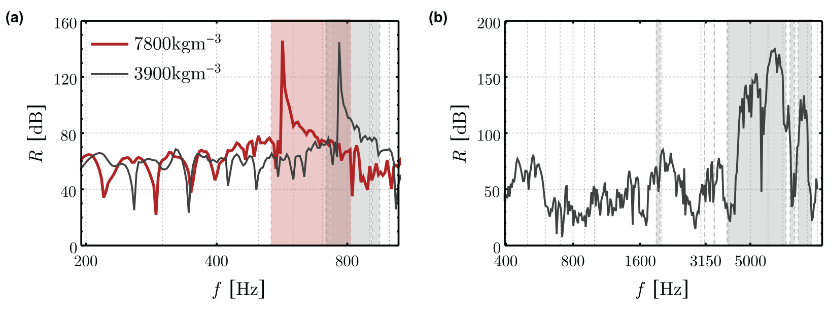
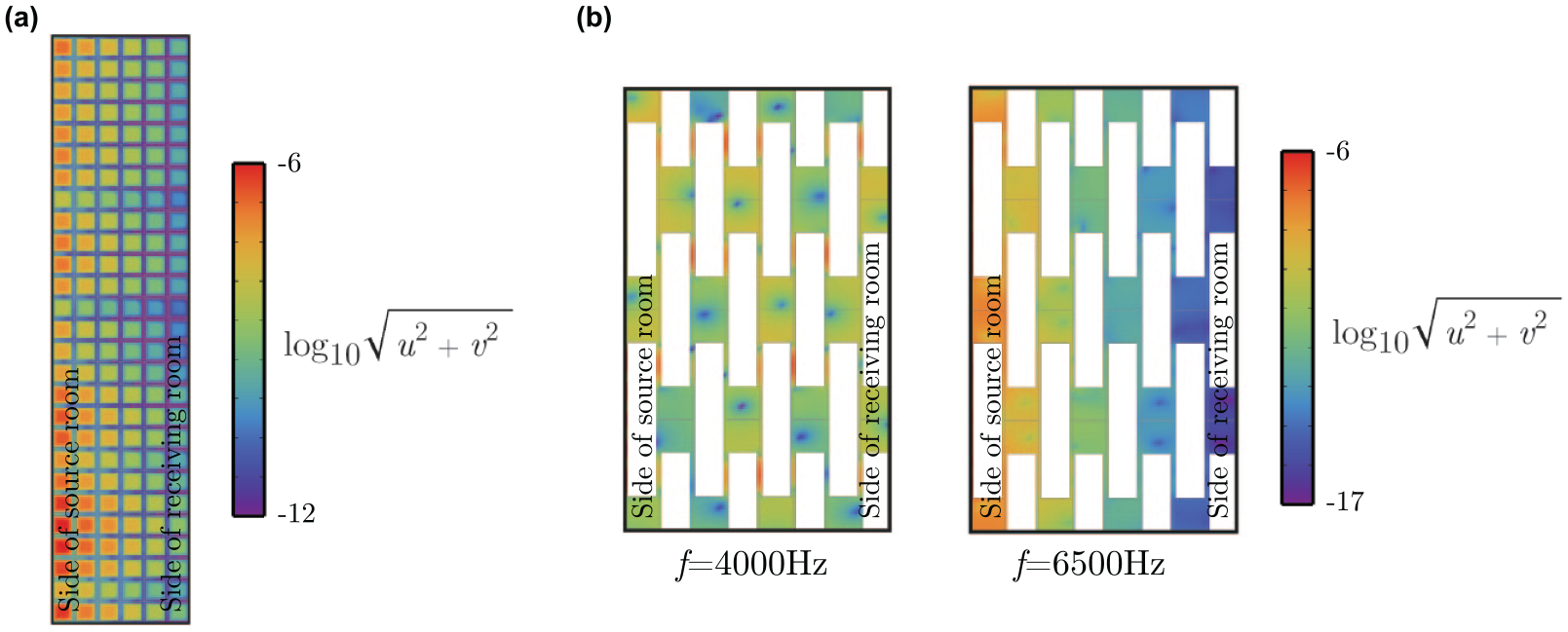
The 2D unit-cell $2_{2D}$ uses a steel core ${\Omega }_m$ coated with a soft elastic material ${\Omega }_i$ $(\rho =1000\mathrm{kg}/{\mathrm{m}}^3,$ $E=0.01$ GPa) and imbedded in a concrete matrix ${\Omega }_a.$ This setup enables vibrations of the core as a local resonator, which allows for a band-gap at relatively low frequencies, as shown in the dispersion diagram in Figure 24(a). The stiffness of the core has very little impact on the band-gap, but a variation of the mass density allows for tuning the first local resonance frequency and shifting the position of the band-gap to a lower frequency. This is shown in the SRI (frequency response) curve in Figure 25(a) for two different mass densities of the core. The Figure 26(a) shows the logarithmic total displacement field at a frequency inside of the band-gap. It can be seen, that the sound insulation relies on the resonance effects of the steel cores, which counteract the wave propagation by their vibrations inside the soft matrix. In the last example, we examine a specifically designed hollow brick, which is arranged according to Figure 20(c). Concrete is used as the material for the hollow brick. Again, the dimensions of the brick $h_a$ , $h_i$ , $w_a$ and $w_i$ are optimized for achieving a wide band-gap at a low frequency while maintaining a rather small thickness of the wall. The dispersion diagrams are shown in Figure 24(b). There is one large band-gap but also several smaller band-gaps exist due to the irregular geometry of the unit-cell. It should be noted here, that a filling inside the cavities (e.g. to improve the thermal insulation) must not affect the wave propagation characteristics, otherwise the band-gaps will be changed. The transmission loss of the brick wall is shown in Figure 25(b) for $n_{pc}=4$ , where the peaks corresponding to the respective band-gaps of the dispersion diagrams can be seen. Due to the overlapping resonance effects and the small width of the band-gaps, some of the peaks are not evidently distinct. Again, the logarithmic total displacement field is shown in Figure 26(b) for a frequency outside and inside of the band-gap.

Figure 24.

(a): Dispersion diagram for the unit-cell $2_{2D}$ with $h_m=0.03375$ m and a steel core. (b): Dispersion diagram for the unit-cell $3_{2D}$ with $w_a=0.5$ m, $h_a=0.075$ m, $w_i=0.35$ m and $h_i=\mathrm{0}\mathrm{.06375}$ m. The gray areas mark the band-gaps.

Figure 25.

SRI curves for (a): the periodic wall composed of the unit-cells $2_{2D}$ with two different values of the mass density of the core (the gray and red areas mark the band-gaps from the calculation of the dispersion diagram, shown for 7800 ${\mathrm{kgm}}^{-3}$ in Figure 24(a)) and (b): the periodic wall composed of the unit-cells $3_{2D}$ (the gray areas mark the band-gaps from the dispersion diagram in Figure 24(b)).

Figure 26.

Logarithmic displacement fields for a representative section of the periodic wall composed of (a): the unit-cells $2_{2D}$ at $f=565$ Hz (within the band-gap) and (b): the unit-cells 3_2D at $f=4000$ Hz (outside of the band-gap) and $f=6500$ Hz (within the band-gap).

Conclusions

In this paper, the acoustic insulation properties of periodically layered walls are analyzed with the help of a virtual acoustic laboratory. To consider the most important physical phenomena, which could occur in a real measurement laboratory, a strongly coupled FSI model is adopted. The governing equations are solved numerically by the SEM to increase the efficiency and accuracy of the calculation. Regarding the efficiency of the SEM, it is found that a rather high accuracy is necessary to precisely determine the sound reduction index, especially at high frequencies. The use of the high-order shape functions decreases the computing time for obtaining the SRI curve over a large frequency range in comparison to the standard FEM.

The periodically layered walls show promising features for special sound insulation applications. These could be relevant to the noise reduction in civil engineering or vibration protection of sensitive measurement instruments in mechanical engineering in a defined frequency range. The increase of the sound reduction index in the frequency range within the band-gaps is extremely high for most of the examined setups. Such a high sound reduction index could not be achieved by traditional monolithic walls, even with a very large thickness. The range of the band-gaps for the studied periodic wall structures in this paper is still limited to relatively high frequencies, and achieving the low-frequency band-gaps while maintaining the high efficiency and feasibility remains a challenging task for practical applications.