Finite element investigations of the fluid-solid behaviour in a bio-inspired poroelastic bearing

Abstract

Poroelastic materials are commonly found in biological systems, such as articulating cartilage, and the ability to predict their biphasic behaviour is a key step in the understanding of joint health and the development of biomimetic devices. Here, a fully coupled three dimensional finite element study is presented to demonstrate the permeability dependent load carrying capacity of fluid pressure in a time-varying poroelastic system. A bio-inspired material model is demonstrated with relaxation simulations which first show results for a cartilage-like sample and then for a variation of permeability from ${10}^{-19}{\mathrm{m}}^2$ to ${10}^{-13}{\mathrm{m}}^2$ . The relaxation rate is non-linear but the total relaxation time scales linearly with permeability. That material model is then demonstrated in the context of a mechanical bearing operating in lubricated contact with an impermeable wall. The results show that for a given set of operating conditions the permeability modifies how the fluid and solid phases accommodate applied loads. High fluid load support varies through the thickness and width of the bearing. It is particularly high around regions where the interstitial flow is restricted by external factors such as contact interfaces. The model offers a novel method to predict local pressures and stresses within a poroelastic material.

Introduction

This research was inspired by the work Prof Duncan Dowson undertook from the 1960s ¹ and later in collaboration with Prof Zhongmin Jin ² on the potential explanation for the ultra-low friction observed in natural joints under operation. These publications aimed to develop a biphasic material model for cartilage (originally derived by Mow ³ ) to investigate the thickness of films formed between cartilage layers in natural joints and explore the friction characteristics of such contacts. Some of the authors of this paper have also been fortunate to have had many fascinating discussions with Duncan on the subject. Duncan’s knowledge provided valuable context and wider perspective to the work presented in this paper and to some of the authors’ other publications.

The tribological effects in naturally occurring poroelastic materials, specifically mammalian cartilage, have been of interest to researchers for several decades.^4,3,5 This spawned an interest in the development of biomimetic lubricating hydrogels. ⁶ The lubrication process at the boundary is complicated by the presence of multiple phases, soft materials and numerous chemical and ionic interactions. ⁷ Despite this complexity, the friction response is tied to the pressurisation of the fluid phase^8–10 which is, itself, maintained through motion induced rehydration. ¹¹ Cartilage, which is avascular ¹² and comprised predominately of water ¹³ , also uses this relative motion for the transport of interstitial fluids. While mathematical theories exist to describe the process at the surface ¹¹ , they have not been extended to cover realistic systems with their three dimensional and time dependant complexity, which is necessary to predict the transport of solutes and address joint health.^14,15 The integration of the surface processes and those within the material body suggest that there are also useful tribological properties that can be exploited in mechanical systems. ¹⁶ However, it remains unclear what role specific material parameters should play in the design of tailored biomimetic devices.

Poroelastic materials are comprised of a solid matrix imbibed with fluid to create a composite material whose bulk properties are different from its individual components. ¹⁷ Compression tests on cartilage samples exhibit large initial load responses that relax over time until the load is only supported by the solid matrix.^18–20 Indentation tests performed on gels reveal a similar behaviour. ²¹ In both scenarios, the transient behaviour is derived from the migration of interstitial fluid along gradients of fluid pressure and molecular concentration. On the macro scale the two mechanisms are analogous, i.e. where the combined materials properties are modified by the fluid phase as it moves through the solid matrix. They differ on the pore scale. In the molecular concentration mechanism the diffusion process follows Fick’s Law and the influence on the matrix is a consequence of molecular interactions and osmotic pressure. In this instance the poroelastic effects are derived from chemical and ionic interactions. ²² In the fluid pressure mechanism the diffusion process follows Darcy’s Law. In this instance the poroelastic properties result from mechanical interactions between the solid and fluid phases that create volumetric fluxes through the porous media. ²³ These fluxes exert a pressure on the network, contributing a stress and increasing the material stiffness. The macro behaviour is not limited to one mechanism; in fact it is often complicated by additional effects such as viscoelasticity. ²⁴

Biot derived an early description of porous media flow. ²³ While it remains commonly used in geoengineering^25,26, it has also been adapted for the analysis of biological systems ²⁷ and gels. ²⁸ These have been expanded to incorporate hyperelastic material models for application to large deformation finite element modelling ²⁹ and have been further expanded by coupling thin-film theory to describe the lubricating boundary.^16,30

This finite element study investigates the biphasic behaviour of a poroelastic bearing inspired by the function of articular cartilage. It focuses on the mechanical origins of poroelasticity, which are derived a Darcy-type diffusion mechanism. The first set of models demonstrate the load induced relaxation response that is characteristic of a poroelastic material. This was done with a simulated cartilage-like material that is comparable to previous experimental studies. After establishing the material model in 3D, it is then applied in the context of a bearing operating in lubricated contact with a smooth wall with the inclusion of a lubricated film when a gap is present. The load responses of the bearing are reported for the solid and fluid phases over a range of permeabilities and geometries.

Methods

The first part of this section describes the poroelastic governing equations for the fluid flow and solid response of poroelastic materials. This is followed by a description of how a typical experimental compression setup is modelled to produce displacement-relaxation and load-relaxation simulations. The final part of this section describes the setup for a poroelastic bearing operating in lubricated contact.

Governing Equations

The poroelasticity is modelled as a biphasic continuum material where the solid phase is coupled to the fluid phase to form a system of partial differential equations.

Solid Phase

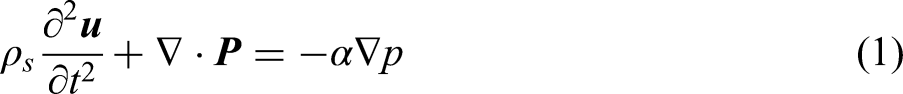
The solid phase is described by the equation for momentum transfer in a continuum 1 and was coupled to the fluid phase with a force derived from the pressure gradient. The first Piola-Kirchoff stress tensor, $\mathit{P}$ in Equation 2, is equal to the derivative of the strain energy density, $W$ , and the deformation gradient $\mathit{F}=\mathit{I}+\mathrm{\nabla }\mathit{u}$ , where $\mathit{I}$ is the identity matrix and $\mathit{u}$ is the material displacement field variable. The first term on the left hand side describes inertial effects where $t$ denotes time and ${\rho }_s$ is the density of the solid phase measured in the absence of fluid. On the right hand side is the coupling term containing the Biot-Willis coefficient ³¹ , $\alpha$ , and the pressure gradient in the fluid phase, $\mathrm{\nabla }p$ . The term represents the stress contribution to the solid phase resulting from fluid motion. The coupling term only produces hydrostatic stresses, and as such does not directly contribute to shear stresses in the solid phase.

$$\rho {}_s\frac{{\mathrm{\partial }}^2\mathit{u}}{\mathrm{\partial }{t}^2}+\mathrm{\nabla }\cdot \mathit{P}=-\alpha \mathrm{\nabla }p$$

(1)

$$\mathit{P}=\frac{\mathrm{\partial }W}{\mathrm{\partial }\mathit{F}}$$

(2)

The strain energy density is given in Equation 3. The components are modified by the Biot-Willis coefficient which varies between 0-1. It expresses the portion of fluid pressure that acts on the solid phase to produce a stress in response to a volume change, with 0 indicating no interaction and 1 indicating a full interaction.

$$W=\alpha W_1+(1-\alpha )W_2$$

(3)

The strain energy density was described by the compressible Neo-Hookean hyperelastic material model where $G$ and $K$ are the shear and bulk moduli of the solid in the absence of the fluid. The right Cauchy-Green deformation tensor is $\mathit{C}={\mathit{F}}^T\mathit{F}$ , the first invariant of which is given by $I_1=\mathrm{tr}(\mathit{C})$ and $J=det(\mathit{F})$ is a measure of the volume change.

$$W_1=\frac{G}{2}(I_1-3-2\ln J)$$

(4)

$$W_2=\frac{K}{2}(J-1{)}^2$$

(5)

Fluid Phase

The interstitial fluid was modelled as the movement of fluid through an interconnect network of pores. This situation is described by Darcy’s law, with pressure as the field variable, and was coupled to the solid phase with the total derivative of volumetric strain. This equation describes the macro-scale permeability of the porous matrix rather than the small scale geometry. This would most likely be extracted from experimental measurements, see for example ¹⁷ who focused on the development of porous materials with properties similar to those encountered in cartilage as is used in this paper. The conservation of mass for flow in the porous media is then given by equation 6.

$$S{\rho }_f\frac{dp}{dt}-\mathrm{\nabla }\cdot ({\rho }_f\mathit{q})=-\alpha {\rho }_f\frac{DJ}{Dt}$$

(6)

The divergence of fluid velocity gives the fluid’s volume change within the material. The velocity was described with Darcy’s equation, $\mathit{q}=-\frac{\kappa }{\eta }\mathrm{\nabla }p$ , which relates the fluid velocity (or flow rate), $\mathit{q}=ϵ(v_f-v_s)$ (where $ϵ$ is the permeability and $(v_f-v_s)$ is the relative velocity of the fluid to that of the solid matrix), to the intrinsic permeability, $\kappa$ , of the solid phase, the viscosity of the fluid, $\nu$ , and the pressure gradient, $\mathrm{\nabla }p$ . The first term describes the transient change in volume where ${\rho }_f$ is the compressible fluid density given by ${\rho }_{f0}\exp (\chi p)$ , ${\rho }_{f0}$ is the fluid density at ambient conditions, $\frac{dp}{dt}$ is the change of pressure with time and $S={ϵ}_0\chi +\frac{(1-\alpha )(\alpha -{ϵ}_0)}{K}$ is the coefficient of poroelastic storage. The coefficient of storage was written in terms of the initial solid porosity, ${ϵ}_0$ , the fluid compressibility, $\chi =\frac{1}{{\rho }_f}\frac{d{\rho }_f}{dp}$ , and the inverse bulk modulus, $K^{-1}$ which is the definition of solid compressibility and is a coefficient of proportionality in the strain energy density. The total derivative term, Equation 7, couples volume changes from the solid phase to the fluid phase.

$$\frac{DJ}{Dt}=\frac{\mathrm{\partial }J}{\mathrm{\partial }t}+\mathit{v}\cdot \mathrm{\nabla }J$$

(7)

The volume changes induced from body translations and rotations are described by the term $\mathit{v}\cdot \mathrm{\nabla }J$ , where $\mathit{v}={\mathit{v}}_{\mathit{T}}+\mathbf{\Omega }\times (\mathit{x}-{\mathit{x}}_{\mathbf{0}})$ is the sum of the two components. Rotation is defined by the vector distance to the centre of rotation, $\mathit{x}-{\mathit{x}}_{\mathbf{0}}$ and the velocity about the axis, $\mathbf{\Omega }$ .

Lubricated Contact Boundary

The lubricated contact boundary refers to the interface between the surface of the poroelastic material and the smooth impermeable wall. The porosity of the solid matrix creates a complicated mix of fluid pockets with points of solid contact on the wall. ³² This was simplified to a thin film where the fluid at the poroelastic surface was assumed to have the same pressure as the film and solid contact occurred where the film was below some critical thickness. In this way the boundary pressures and stresses where simplified into a lubricated contact condition that derived fluid pressures from the lubricant film and solid stresses from contact mechanics.

The contact problem was addressed with the penalty method, Equation 8. This method applies a “penalty” load to the poroelastic surface based on the gap, $h$ , separating it from the impermeable wall. The load grows exponentially as the gap approaches zero and deforms the poroelastic material in the contact region such that it complies to the rigid wall, preventing surface overlap. There remained an extremely small minimum gap, which in the case of the bearing model was $(\approx {10}^{-7}\mathrm{m})$ . This gap was a consequence of the penalty formulation.

$$L_{pen}={\beta }_1\times {10}^{({\beta }_2(h-h_{min}))}$$

(8)

The penalty load, $L_{pen}$ , was applied on the lubricating boundary by setting it equal to the normal boundary stress, $(\mathit{P}\cdot \mathit{n})dA=L_{pen}$ , where $dA$ is the discrete boundary area. The coefficient ${\beta }_1$ is equal to one and has units of Newtons, ${\beta }_2$ describes the steepness of exponential growth and $h_{min}$ is an offset that ensures the exponential growth becomes large before the gap reaches zero. Together these terms should be formulated to prevent surface overlap (i.e. a negative gap) at all anticipated loads with ${\beta }_2$ taking a very large value and $h_{min}$ taking a small one.

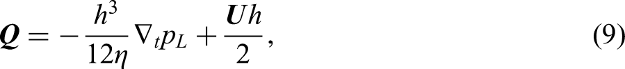
The layer of lubricating fluid was assumed to follow thin film theory. In this instance the fluid pressure in the film is described with the Reynolds equation which governs the pressure distribution in thin viscous films and is commonly used to describe lubricating problems. ³³ It assumes that the film thickness is much less than its length, viscous forces are much larger than inertial forces and that pressures are constant through the thickness of the film. Flux through the film is then given by Equation 9,

$$\mathit{Q}=-\frac{h^3}{12\eta }{\mathrm{\nabla }}_t{p}_L+\frac{\mathit{U}h}{2},$$

(9)

where $h$ is the distance separating the bearing surface and the impermeable wall, $\mathit{U}$ is the surface speed of the bearing and $p_L$ is the pressure in the lubricating film. The surface tangent gradient operator, ${\mathrm{\nabla }}_t$ , was assessed on the lubricating surface. Mass conservation in the thin film is related to the bearing material because fluid can migrate across the lubricating boundary 10.

$$\frac{\mathrm{\partial }({\rho }_{f}h)}{\mathrm{\partial }t}+{\mathrm{\nabla }}_t\cdot ({\rho }_f\mathit{Q})={\rho }_f\mathit{q}\mathbf{\cdot }\mathit{n}$$

(10)

The lubricating mass flux within the thin film is given by ${\mathrm{\nabla }}_t\cdot ({\rho }_f\mathit{Q})$ . The time dependant change in film thickness is give by $\frac{\mathrm{\partial }h}{\mathrm{\partial }t}$ , and leads to a scenario where fluid is either pressed into the material when the surfaces approach or is extracted as they separate. This normal flux is $\mathit{q}\mathbf{\cdot }\mathit{n}$ , where $\mathit{n}$ is the outward facing unit normal on the lubricating boundary.

Numerical Formulation

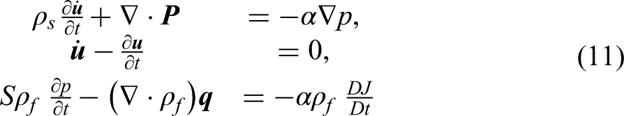
The open source finite element software FEniCS^34,35 was used to perform the simulations in this study. The dynamic terms in the momentum equation were reduced to first order by the substitution $\frac{\mathrm{\partial }\mathit{u}}{\mathrm{\partial }t}=\dot{\mathit{u}}$ . The problem then required three field variables in a mixed displacement-velocity-pressure formulation ( $\mathit{u},\dot{\mathit{u}},p$ ) and resulted in the system of equations shown in 11.

$$\begin{array}{cc}\rho {}_s\frac{\mathrm{\partial }\dot{\mathit{u}}}{\mathrm{\partial }t}+\mathrm{\nabla }\cdot \mathit{P}& =-\alpha \mathrm{\nabla }p,\\ \dot{\mathit{u}}-\frac{\mathrm{\partial }\mathit{u}}{\mathrm{\partial }t}& =0,\\ S{\rho }_f\frac{\mathrm{\partial }p}{\mathrm{\partial }t}-(\mathrm{\nabla }\cdot {\rho }_f)\mathit{q}& =-\alpha {\rho }_f\frac{DJ}{Dt}\end{array}$$

(11)

The geometry was discretised with second order tetrahedral elements in the displacement field and first order tetrahedral elements for the velocity and pressure fields. The time domain was discretised with a backward Euler (implicit) time-stepping method.

Relaxation Simulations

In biological engineering, cartilage is often approximated as a biphasic poroelastic material and its properties are commonly quantified using a combination of displacement-relaxation and load-relaxation tests. In biological fields the load tests are sometimes called creep tests. Here, the load-relaxation terminology was used to avoid confusion with creep phenomena that refer to viscoelastic effects. These tests are used to determine the solid (aggregate modulus) and fluid (permeability) properties^19,18,36 and are similar to indentation tests.^37–39 In the procedure, the sample is compressed in a confined chamber with a piston that has a porosity much larger than the test sample. The internal fluid pressure is initially equal to the ambient pressure, $p=0$ . When loaded, the fluid pressure increases and exudes out through the porous piston as shown in Figure 1.

Figure 1.

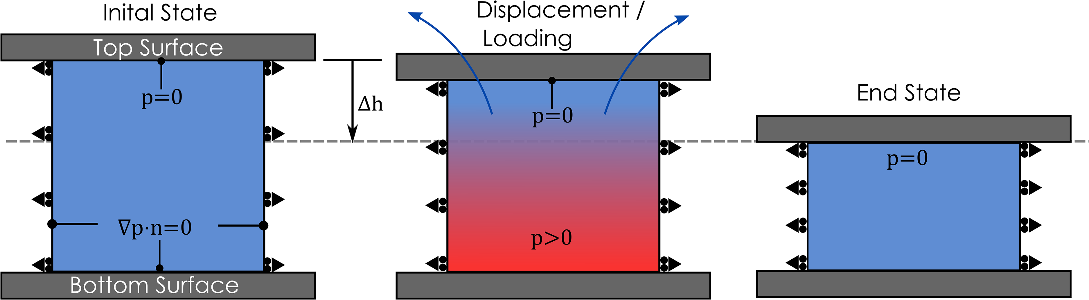
Displacement-relaxation and load-relaxation geometry at three different phases of the test. The simulation was in three dimensions, but the schematic was simplified to two dimensions. The top surface is rigid and porous such that it offers no resistance to the fluid. The displacement-relaxation test displaces the top surface by $\mathrm{\Delta }$ h. The load-relaxation test applies a fixed load to the top surface. Displacement is constrained in the transverse axis but free in the vertical axis. Both simulations end when fluid pressure returns to zero.

Both tests were simulated using the material model described in the Governing Equations section which was applied to a $1\mathrm{mm}\times 1\mathrm{mm}\times 1\mathrm{mm}$ cube of material. The bottom surface was fully constrained and sealed, $\mathrm{\nabla }p=0$ . The vertical sides were also sealed but constrained such that only vertical motion was allowed. At the top surface the pressure was set to zero to approximate the porous piston.

Displacement-Relaxation Procedure

The displacement-relaxation simulation displaced the top surface by $10\text{\%}$ of the sample’s total height at a rate of $0.25{\mu \mathrm{ms}}^{-1}$ . The displacement of the top surface was set with a Dirichlet boundary condition that was updated at each time-step. Once complete, the top surface was held while the fluid pressure dissipated resulting in the load in the surface due to the elastic solid load only.

Load-Relaxation Procedure

The load-relaxation tests applied a constant load resulting in a $10\mathrm{kPa}$ normal stress on the top surface and measured the resultant displacement. The test ended when the fluid pressure returned to zero and the load was entirely supported by the solid phase. The load was applied as a Neumann traction condition. The simulation was first setup to represent a cartilage-like material with an intrinsic permeability of $\kappa =5\times {10}^{-19}{\mathrm{m}}^2$ . A subsequent parametric variation of the intrinsic permeability was conducted to demonstrate its relation to dissipation rate in the absence of confounding boundary and operating conditions that were present in the bearing model (described in the following section).

Procedure for the Bio-Inspired Bearing Simulation

The bearing was inspired by articular cartilage in which the poroelastic material is fixed to rigid cortical bone while its surface slides in lubricated contact with an opposing cartilage layer. Here the configuration reflected a mechanical bearing and the opposing cartilage surface was replaced with a smooth impermeable wall. This layout, with the boundary labels, is described in Figure 2. The poroelastic lubricating surface is free to deform and open such that fluid can flow between the poroelastic material and the thin lubricating film. The entire bearing is submerged in a fluid bath which also allows fluid exchange to occur at the side walls. The bearing geometry is ring-shaped, a ${80}^{\circ }$ section of which is used for the simulation domain. The bearing was set to operate at a steady rotation of $1\frac{rad}{s}$ and was compressed to a depth of $0.1\mathrm{mm}$ against a smooth impermeable wall to form a lubricated contact region. The permeability of the poroelastic material was varied over a range of ${10}^{-16}{\mathrm{m}}^2$ to ${10}^{-13}{\mathrm{m}}^2$ to demonstrate the relation between the fluid load support and the permeability.

Figure 2.

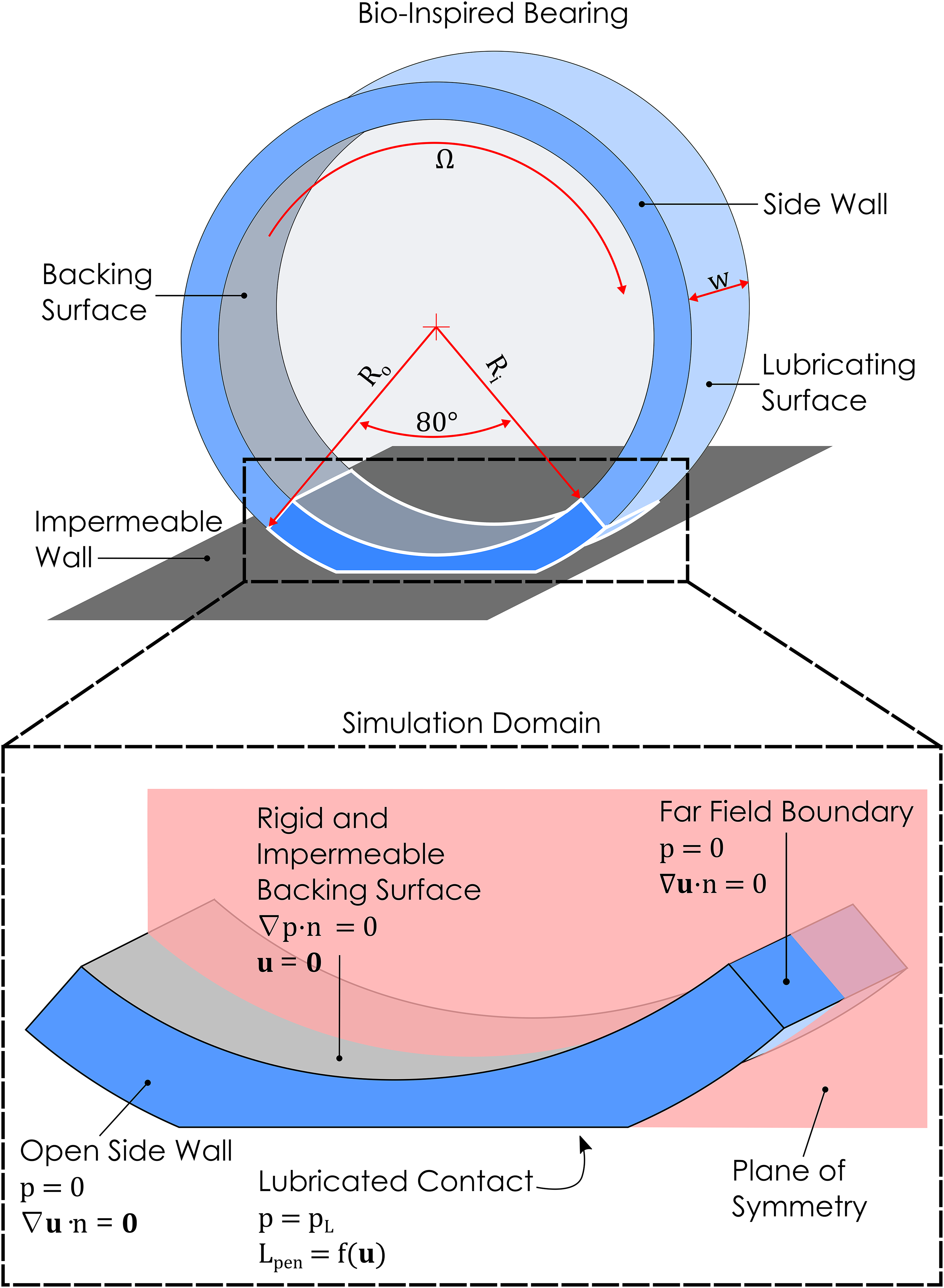
The bearing geometry (top) is shown rotating at angular velocity $\mathrm{\Omega }$ in lubricated contact with the impermeable wall. The expanded region shows the simulation domain. The backing surface is rigid and impermeable. The side walls are unconstrained and have an open fluid boundary. The lubricating surface is constrained with the contact load on the displacement field and with the lubricating pressure condition on the pressure field. The simulation section spans an ${80}^{\circ }$ segment and is highlighted with a white border. $R_o$ and $R_i$ are the outer and inner radii respectively, and $w$ is the width of the bearing.

The contacting boundary made the problem numerically stiff such that a start-up procedure was required. This relied on continuation methods, where the simulation began in a relatively simple part of the design space and was progressively manipulated into the desired design space. This type of method has been commonly employed to solve boundary value problems which require an initial state to be given. Here, the start-up condition was an un-deformed bearing with a large permeability, $\kappa ={10}^{-13}$ , rotating far from the wall such that there was no contact contribution. Using time-stepping, the bearing was moved into contact and compressed. The large permeability minimised the effects of the coupling terms in Equations 1 and 6. The process kept the problem numerically stable.

Results and Discussion

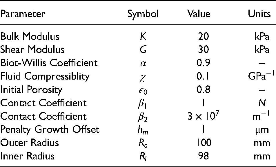
The results were broken into sections addressing the relaxation and bearing studies. The parameters used in the simulations are shown in Table 1.

Table 1.

Material properties used for all simulations. The contact and geometric terms are relevant only to the bio-inspired bearing model.

Parameter	Symbol	Value	Units
Bulk Modulus	$K$	$20$	kPa
Shear Modulus	$G$	$30$	kPa
Biot-Willis Coefficient	$\alpha$	$0.9$	–
Fluid Compressiblity	$\chi$	$0.1$	GPa ${}^{-1}$
Initial Porosity	${ϵ}_0$	$0.8$	–
Contact Coefficient	${\beta }_1$	$1$	$N$
Contact Coefficient	${\beta }_2$	$3\times {10}^7$	${\mathrm{m}}^{-1}$
Penalty Growth Offset	$h_m$	$1$	$\mu \mathrm{m}$
Outer Radius	$R_o$	$100$	mm
Inner Radius	$R_i$	$98$	mm

Displacement and Load Relaxation

The relaxation tests are presented as a demonstration of the transient nature of the poroelastic material behaviour under load and displacement. The aggregate modulus, $M$ , is an elasticity measure often determined from an experimental relaxation test. ¹⁹ Here a value of 0.6  MPa was adopted and was paired with a fluid viscosity of $0.001Pa\cdot s$ to represent a cartilage-like material. The aggregate modulus was converted to the shear and bulk moduli using Equations 12 and 13 for use in the finite element model. This required a known Poisson’s ratio, $\nu$ , for the solid matrix, which was assumed to be zero. This assumption was arrived at by considering the solid matrix in the absence of fluid. In this scenario the material contains empty voids in an arbitrary configuration which, when loaded, allows the material to collapse into them yielding no transverse change in volume.

$$K=\frac{M(1+\nu )}{3(1-\nu )}$$

(12)

$$G=\frac{M(1-2\nu )}{1(1-\nu )}$$

(13)

for $\nu =0$ , $K=\frac{K}{3}$ and $G=M$ .

Displacement-Relaxation

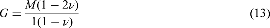
The displacement-relaxation results are shown in Figure 3. The displacement phase lasted 400 seconds during which the fluid pressure on the bottom surface and the solid stress on the top surface increased non-linearly with a decaying gradient. Both maintained similar values throughout the loading phase. The solid stress on the backing surface also increased but at a lower rate, reaching 13  kPa during the loading phase. After displacement, the sample was held statically and the fluid continued to diffuse through the material and out of the top surface. This correlated to a pressure drop which was steepest immediately after displacement and decayed towards zero over 3500 seconds. The solid stresses on the top and bottom surfaces converged to a value of 57  kPa, at which point the fluid pressure had fully dissipated, indicating that the load was carried entirely by the solid phase. In this end state, the reactive force is equal to that of a sample in which all the fluid has been evacuated.

Figure 3.

Displacement-Relaxation (a) and Load-Relaxation (b) results for the cartilage-like model. The bottom surface (BS) is constrained so there is no displacement and no fluid can pass through. The top surface (TS) is open so fluid can diffuse out of the poroelastic material. This open boundary was created by setting the pressure boundary condition to zero. The insert in part a is used to show the asymptotic convergence of the solid stress on the top and bottom surfaces.

Throughout the early portion of the test, where possible, the fluid phase supported most of the load. This was not possible at the open top surface. The displacement deformed the solid phase and the pressure rose in response to the volume change. The fluid in the pores was then driven along the pressure gradient, towards the open top surface. For the fluid pressure to build up there needed to be some mechanism to restrict its flow. This was only present at the bottom surface and on the sides where the walls were impermeable.

The results in 3 are persistent in the literature where authors have found similar loading profiles ¹⁸ and loading magnitudes with surface specific loads.^19,40 In these cases the fluid pressure was experimentally shown to decay asymptotically towards zero. This is a general result for cartilage and has been shown to hold for step ⁴¹ and indentation ⁴² loading scenarios.

The rate of fluid pressure dissipation is mathematically related to the coupling terms in Equations 1 and 6 which determines the solid stress contribution from the fluid pressure gradient as only a fluid in motion contributes a stress. Hence, even after the stress on the top and bottom surfaces had converged, highlighted with the insert in Figure 3a, there remained a nearly stationary fluid in the pores.

Load-Relaxation

The load-relaxation results are shown in Figure 3(b). The 100 kPa load was initially held primarily by the fluid phase at the bottom surface and entirely by the solid phase at the top surface. Similar to the displacement-relaxation test, the fluid pressure dissipated over time as load was transferred to the solid phase. Gradients were steepest in the early phase of the test and asymptotically decayed. The process was essentially complete after 7000 seconds. Start-up effects can be seen in all three data points as the load was instantaneously applied, creating momentary inertial effects.

The rate of fluid dissipation dictated the shape of the curves in both the displacement and load relaxation tests. The rate is governed by the Darcy component of Equation 6, $\frac{\kappa }{\eta }\mathrm{\nabla }p$ , which contains the intrinsic permeability of the solid phase, $\kappa (m^2)$ , and the viscosity of the fluid phase, $\eta (Pa\cdot s)$ . The dissipation rate has a non-linear relation to these properties, but the total time taken to dissipate is linearly related. This was demonstrated in Figure 4, where the intrinsic permeability was varied from ${10}^{-19}{\mathrm{m}}^2$ to ${10}^{-13}{\mathrm{m}}^2$ which is approximately the same as cartilage ¹⁹ to soil.^43,44 The permeability was assumed to have no confounding impacts on the material properties of the solid phase and therefore resulted in an equal displacement of the top surface, Figure 4a. In real systems the deformation would bring about a change in the permeability of the solid phase as the porous channels collapsed. A number of material specific studies have investigated this process.^45,44

Figure 4.

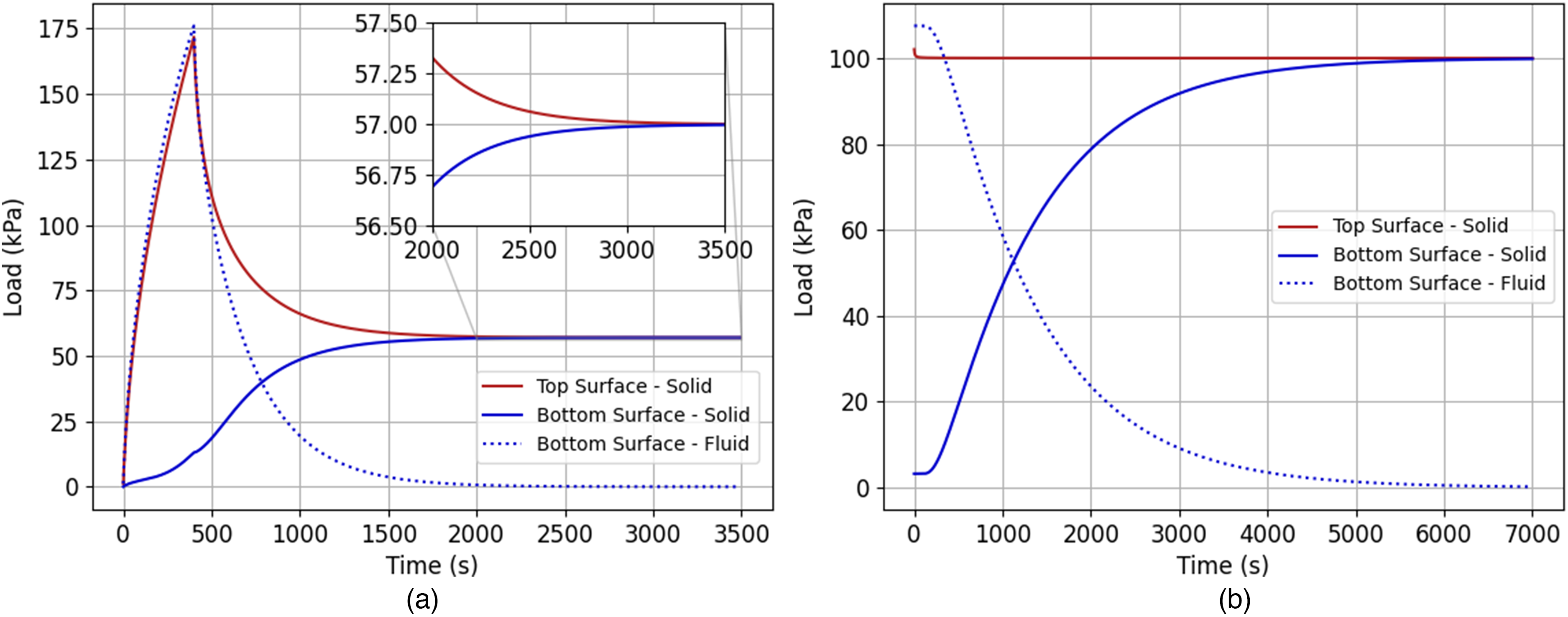
Results from the parametric variation of the permeability in the load-relaxation test. The displacement (a) of the top surface and the fluid pressure (b) acting on it.

The utility of Figure 4 is to show that the critical timescales depend on the permeability and viscosity. A biphasic material subjected to a load would appear incompressible, or nearly so, on short time scales. While on long time scales, where the volume change was gradual, the pressure response would be negligible.

The simple design of these tests demonstrate that the pressure follows an asymptotic decay in response to an applied load. The total time for pressure to dissipate is linearly related to the term $\frac{\kappa }{\eta }$ in the Darcy equation. In the subsequent section this linearity only holds for the permeability term because the fluid viscosity is also present in the Reynolds lubrication equation.

Bio-Inspired Bearing

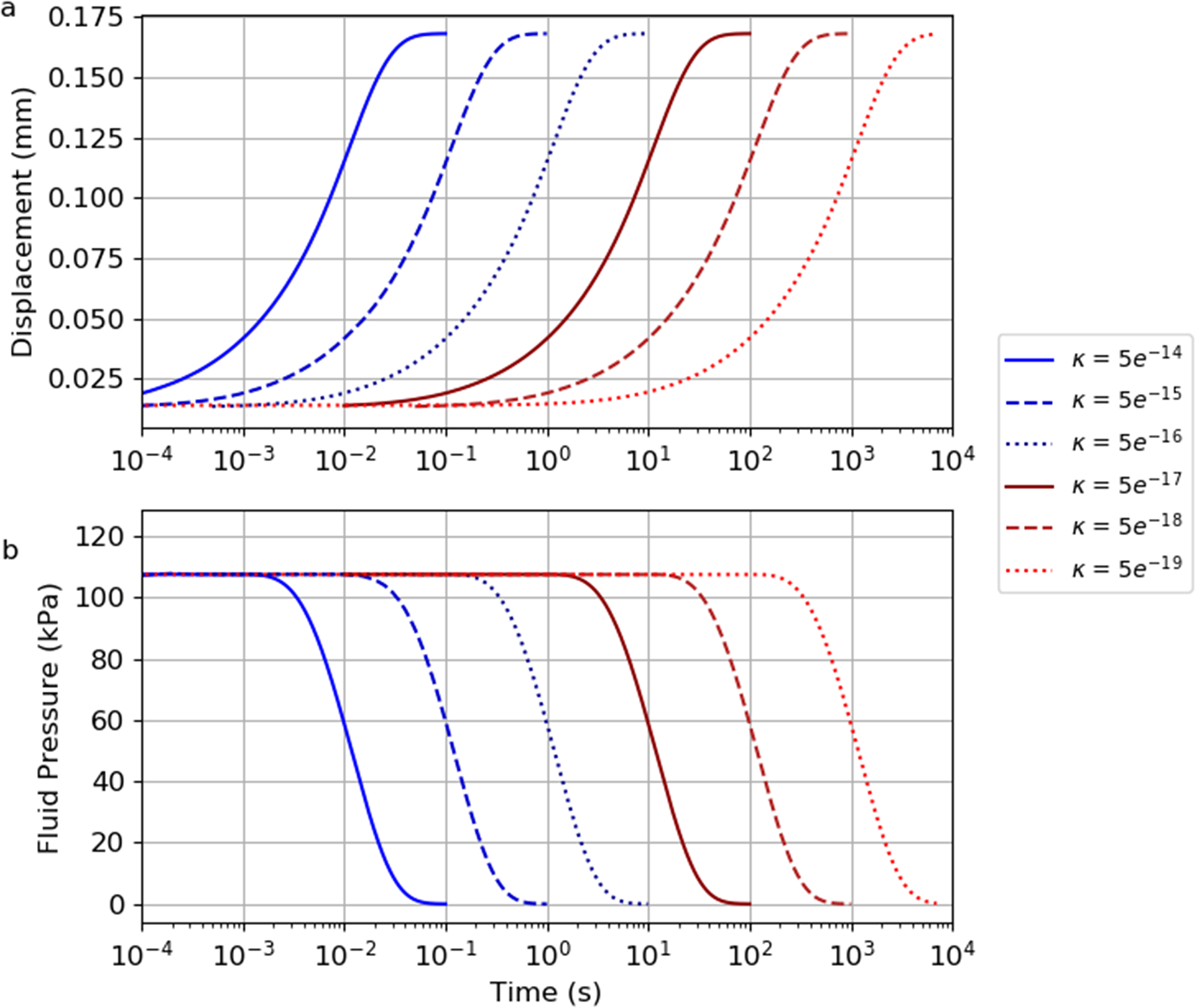
The loading components of the parametric permeability study are shown in Figure 5. The permeability was plotted logarithmically on the x-axis and the load carried on the y-axis. Separate lines were used to show the fluid and solid loads acting on each surface (i.e. backing and lubricating surfaces). The fluid pressure and normal component of the solid stress were calculated by integrating along their respective surfaces to give the total reaction load.

Figure 5.

Results of the parametric permeability study showing the relative load of the fluid and solid phases at the Backing Surface (BS) and Lubricating Surface (LS). The bearing was 2 mm thick by 3.5  mm wide. The numbers and associated colour bars identify the regions discussed in the text.

Unlike the previous cases of a loaded poroelastic component with either a constant force or displacement, the bearing cases considered in this section are all steady analyses. The origin of the volume change for these steady cases is the rotation of the poroelastic material in and out of the contact. This is described by the directional derivative term which is the second right hand side term in equation 7.

Figure 5 contains three distinct regions which are marked with numbered bars. The first is on the left hand side of the plot where permeability is small. In this region the fluid pressures are large and change gradually with permeability. The second is a transition region in which changes in permeability elicit a large change in fluid pressure. The third is the final region on the right hand side of the graph where permeability is large and fluid pressures are low.

In the first region the solid matrix strongly inhibited the free flow of fluid. When the material was deformed, large internal pressure gradients were generated. These gradients interacted with the solid matrix to generate a hydrostatic stress, a result of the coupling term in Equation 1. The backing surface experienced larger fluid and solid loads than the lubricating surface. In this region the coupled interaction between the solid and fluid was large and both phases made important contributions to the macro load response of the material.

The second region was in transition from a state where volume changes produced a large response in the fluid pressure to a state where volume changes produce only a small change in the pressure field. The transition region spanned approximately ${10}^{-15}{\mathrm{m}}^2$ to ${10}^{-13}{\mathrm{m}}^2$ . In this region the fluid pressure was dependant on the permeability. The pressure on the lubricating surface was larger than that on the backing surface for most of this region. In the solid phase, the stresses were initially larger on the lubricating surface but inverted near a permeability of $4\times {10}^{-14}{\mathrm{m}}^2$ . Changes in the stress field were smaller than those seen in the pressure field.

In this region the permeability was so large that fluid flowed easily through the solid matrix in response to deformation and the resulting pressure gradients were small. In Figure 5 this was near $\kappa ={10}^{-13}{\mathrm{m}}^2$ and would have extended to larger values. The coupling terms in equations 1 and 6 were small resulting in a pressure gradient that generated a negligible stress. The majority of the load was carried by the solid phase. In this circumstance the material was tending towards a mono-phasic material governed by solid mechanics.

The fluid pressurisation was a result of the fully hydrated material rotating the contact region where it was compressed against the wall. The operating conditions set the rotation rate and the compression depth. The bearing was rotating at 1  rad/s against the impermeable wall such that the maximum deformation was approximately 0.1 mm or $5\text{\%}$ strain in the centre of the contact area. The rotation introduced a constant source of deformation. This meant that the displaced volume was largely constant throughout the study (note that there were small elastohydrodynamic and poroelastic effects at the lubricating surface that prevented the volume being precisely constant). Therefore in region one, the permeability was sufficiently low to allow the fluid pressure to build up while it passed through the contact region. In region three, the permeability was so large that the fluid pressure easily dissipates within the time taken to traverse the contact region.

Solid and Fluid Behaviour in the Contact Region

The development of the stress and pressure fields as a function of permeability are shown in Figure 6, where permeabilities were selected from the three regions in Figure 5 to depict the transition from a state where the fluid load support was low ( $\kappa ={10}^{-13}{\mathrm{m}}^2$ ) to one where it was high ( $\kappa ={10}^{-16}{\mathrm{m}}^2$ ). The first row shows the fluid pressure field and the second row shows the von Mises stress field in the solid phase. The third row shows the displacement magnitude field plotted on the whole bearing geometry. A gray box was added along the centre/symmetry line. The first two rows show the outline of this box which is 20  mm long and located such that a central cross-section of the contact region is exposed. In the figure the bearing is rotating at $0.1\frac{rad}{s}$ which means that a point entering on the right hand side of the box takes $0.2$ seconds to travel the length of the box. On the right hand side of the box, material rotates into the contact region and is referred to as the upstream while material on the left hand side, where material exits is referred to as the downstream.

Figure 6.

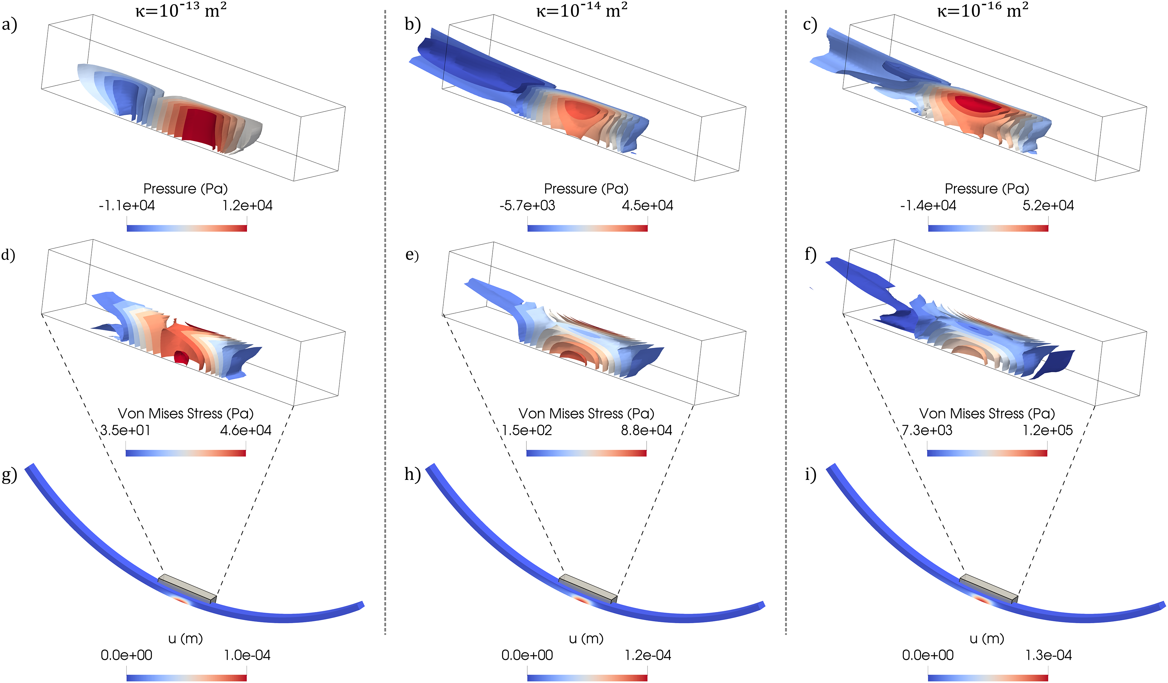
Isosurface plots of the pressure (a,b,c) and von Mises stress (d,e,f) fields. For context, the bottom row (g,h,i) shows the displacement field of the entire geometry with a grey box highlighting the zoomed in region used in the other plots. The zoomed in region also bisects the geometry to show a cross-section along the centre-line of the bearing. The columns correspond to Figure 5 at $\kappa ={10}^{-13}$ , $\kappa ={10}^{-14}$ and $\kappa ={10}^{-16}$ from left to right respectively. In all plots the bearings are rotating clockwise.

Considering the first column of Figure 6 in which the permeability is large, at $\kappa ={10}^{-13}{\mathrm{m}}^2$ . In this state the fluid load support is low. The maximum pressure is 12  kPa, which was the lowest of the three states shown, and the isosurfaces indicate that there is minimal change through the material thickness. Similarly, in the stress field, the range is small and the isosurfaces have minimal variation through the thickness. The isosurfaces both upstream and downstream formed two well defined regions. At the upstream region where the material rotates into contact and the matrix is compressed, creating a pressure increase, and a downstream region where the material rotates out of contact and the matrix expands to its original shape creating a sub-ambient pressure region. In the compressive zone fluid is exuded, primarily out of the side walls as shown by the tight packing of isosurfaces, and is re-absorbed downstream in the expansive zone. The short profile of the expansive zone indicates that the re-absorption occurs quicker than the translation effects of the rotating material. Lubricant cavitation is not considered here, but cavitation and inlet starvation, along with incomplete rehydration of the poroelastic material all need further exploration.

In the second and third columns of Figure 6 the permeability is small enough for pressure gradients to form through the thickness of the material. In 6b and 6c the pressure isosurfaces radiate out from the centre of contact and expand as they approach the backing surface where fluid pressures are high enough to support the majority of the load. On the lubricating surface the solid stress is relatively large, with the isosurfaces also focused around the centre of contact. Comparing these two surfaces illustrates how the fluid and solid phases accommodate applied loads. At the backing surface the fluid is constrained, allowing large pressures to build up. On the lubricating surface fluid can flow into the thin film and, therefore, is constrained only in relation the local film pressure.

The behaviour of the interstitial fluid is governed by Darcy’s equation, in which the direction is derived from the gradients of pressure. The isosurfaces of pressure in Figure 6 show that these gradients were steep in the width direction indicating that fluid was being forced out of the side walls and reabsorbed downstream. In an analogous cartilage system this fluid exchange would occur at the lubricating boundary. ¹¹ Both processes are a consequence of the differential pressure between the external and interstitial fluids. The sub-ambient pressure regions in Figures 6b and 6c are an indication that the material was locally dehydrated and was drawing in fluid from the bath.^46,6 The region increased in length and reduced in pressure as the permeability decreased. With the aid of Figure 4, the dissipation rate in Figures 6b and 6c could be estimated as one to two orders of magnitude smaller than that in 6a. It therefore took longer for the dehydrated region to return to ambient pressure which appeared to “stretch” the region at lower permeability. This meant that in Figures 6b and 6c the re-hydration rate was significantly slower that the translation of the rotating material.

Figures 6g, 6h and 6i show that the maximum deformation increases as permeability decreases. This was because the pressure in the thin film was related to the loads in the bearing. The thin film pressure acts normally to the surface creating a reactionary force that contributed to the displacement, an elastohydrodynamic effect which has also been found in other work. ¹⁶

Taken as a whole, Figure 6 shows how fluid load support develops at different permeabilities. The fluid pressures built-up around regions where the fluid was confined. The most confined fluid was at the backing surface where it could not escape into the surrounding fluid bath. The fluid was partially confined on the lubricating surface because of the contact and large pressures in the fluid film. Interstitial fluid was primarily exchanged at the side walls, creating the three dimensional contours shown in the isosurface plots.

Bearing Width and its effect on Relative Phase Loading

The bearing side walls created a balance between the interstitial fluid pressure and the bath. This effect is explored with the aid of Figure 7 where three bearings of width 1.75mm, 3.5mm and 7mm are compared. In each case the thickness and operating parameters were held constant. The fluid pressures and normal solid stresses were integrated along each surface to give the component loads which were plotted against the change in permeability. The loads were presented in N/(mm of width) to make them comparable. Figure 7d showed the ratio of fluid load to solid load on each surface for each of the three bearing cases.

Figure 7.

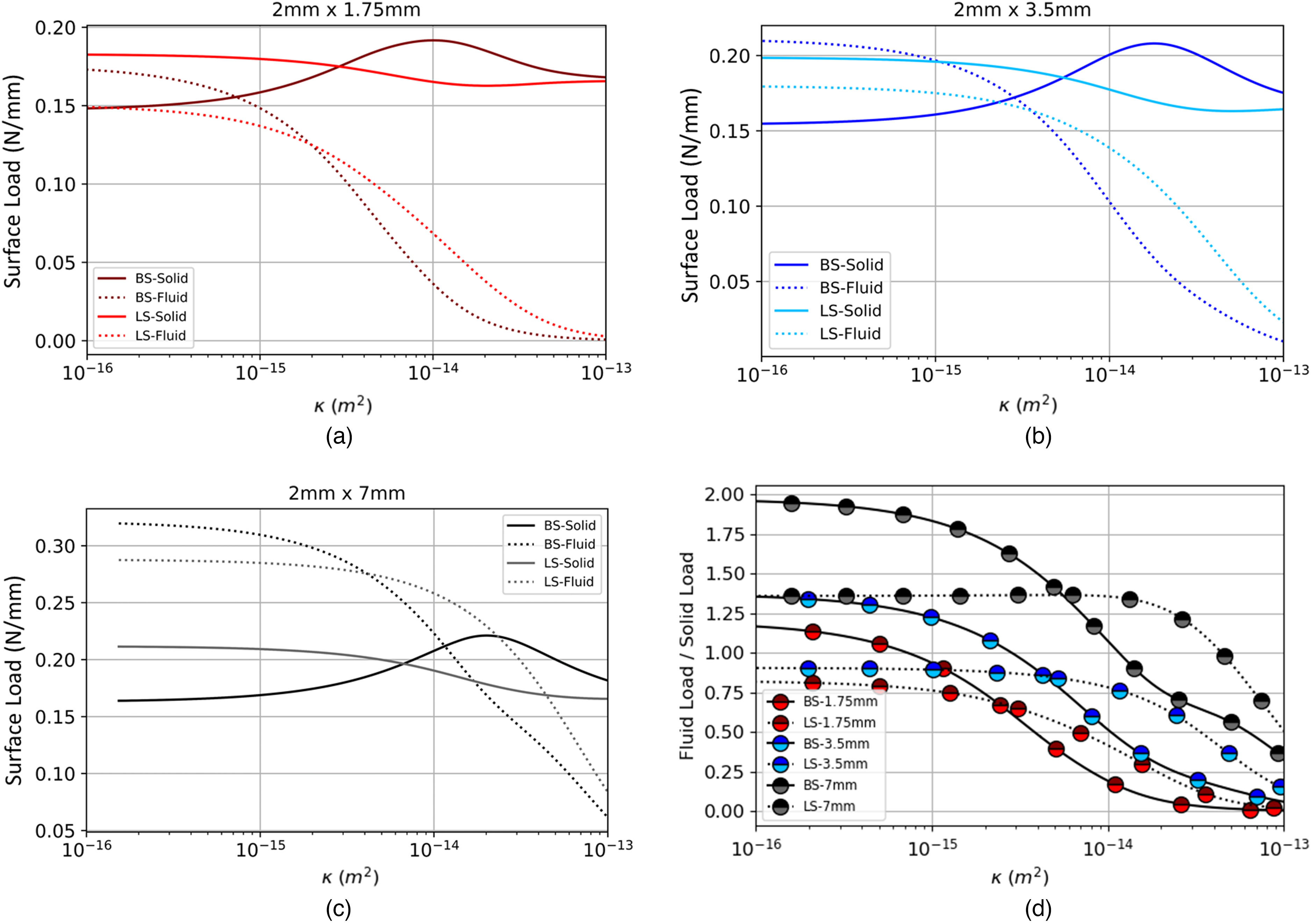
Plots a, b, c are of surface loads, displayed in newtons per millimeter width, recorded at bearing widths of 1.75mm, 3.5mm and 7mm. Plot d is comparative of the other three figures with its vertical axis displaying the fluid to solid load ratio. The abbreviations BS and LS refer to the Backing Surface and Lubricating Surface respectively.

An increase in bearing width increased the fluid load support per unit width across the whole permeability range. It also moved the window for the transition region to larger permeabilities. This was shown as a rightward shift when Figures 7a, 7b and 7c are viewed in sequence. The apparent shift was an indication that the additional material between the centre of pressure in the bearing and the open boundary was applying resistance to fluid, allowing for pressurisation. In all three cases the bearings went through regions which were similar to those labelled in Figure 5.

The ratio of load supported by the fluid to that supported by the solid increased with the bearing width. This increase was facilitated by the ability of the bearing to generate larger fluid pressures. This effect is shown in Figure 7d, where the ratio of fluid to solid load increases with decreasing permeability. In all three cases the ratio was larger at the backing surface than the lubricating surface due to the confinement form the zero flux condition.

The rise in maximum fluid pressure was a result of the increasing separation between the side wall and the high pressure in the contact region. This was illustrated with Figure 8 which showed the backing surface of the 7 mm wide bearing at $\kappa ={10}^{-15}{\mathrm{m}}^2$ . The pressure dropped from a maximum of 82 kPa to zero at the side wall. The side wall condition also forced all the load through the solid matrix. This secondary effect formed a “ring” around the centre of contact. These edge effects were also visible in Figure 6 where they formed tightly packed isosurfaces where the side wall and backing surface meet.

Figure 8.

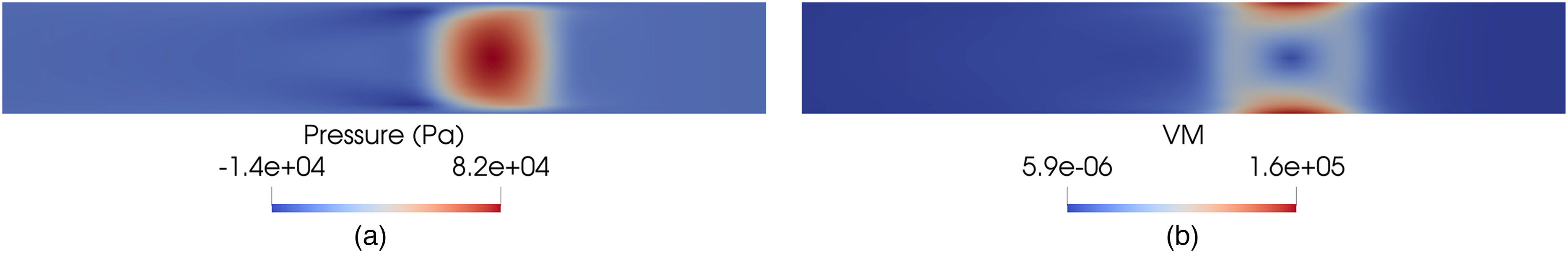
A diagram comparing the pressure contours (top) and von Mises stress contours (bottom) on the backing surface of the 7mm width bearing with a permeability of $\kappa ={10}^{-15}$ .

In a similar way that Figure 4 showed that permeability affected the critical time scale, the bearing width demonstrated that poroelastic materials also have critical length scales. Here, changing the bearing width also changed the distance from the centre of pressure to the side walls. This longer diffusion path increased the peak pressure by giving the pressure gradient a longer distance over which to act. Different combinations of time and length scales describe a huge range of poroelastic-type problems. Biological systems on the cartilage length scale ( $\approx mm$ ) have a permeability near ${10}^{-19}$ which results in pressure diffusion times on the order of minutes to hours. ¹⁹ At the other extreme, where distances are measured on the kilometer length scale, geomechanical phenomena with a much larger permeability ( $\ge {10}^{-13}{\mathrm{m}}^2$ ) operate on diffusion times measured in days to weeks.^43,26

Summary and Conclusion

In this research a hyperelastic material model was coupled to a Darcy porous fluid flow to create a biphasic model which successfully predicted finite deformation of the the solid and fluid phases. The bearing model drew inspiration from articular cartilage, in which a biphasic layer is bounded by a rigid impermeable bone and a lubricating interface. This required the biphasic model to be coupled to the Reynolds lubrication equation and a penalty contact condition. While articular cartilage has evolved to accommodate static, impact and cyclic loads the bearing model presented here considered a constant rotational speed, a situation more commonly found in manufactured bearings.

In a poroelastic system where the fluid-solid interactions arise from volume fluxes, the rate of fluid diffusion is related to the permeability of the solid matrix and the viscosity of the fluid. The response to loading is non-linear and contains an asymptotic decay with respect to the fluid pressure, whereas the time taken for complete diffusion of fluid pressure is linearly related to the permeability and viscosity. This presents a convenient tuning parameter for manufactured poroelastic bearings. In the most common naturally occurring systems the fluid is primarily water-based and the variation of viscosity is small. However, there are examples that have vastly differing permeabilities. This paper demonstrates that a material with soil-like permeability had a pressure diffusion time on the order of ${10}^{-1}\mathrm{s}$ while a cartilage-like permeability takes an order of ${10}^4\mathrm{s}$ . The bio-inspired bearing model was used to explore how a subset of permeability modified the behaviour of a complex system. The model showed diffusion processes could be transported downstream to create sub-ambient regions where fluid was drawn into the material from the external bath far from the contact region. This indicated the presence of strong three-dimensional features that have not been observed or captured before in previous models.^16,30

Fluid-load support is the portion of the total load applied to a material that is supported by the fluid phase and it is critical in determining the tribological properties of cartilage. ¹⁰ This has been primarily of interest for sliding interfaces where fluid pressures offset the loads that would be carried by the solid matrix thereby minimising the friction from solid-on-solid interactions.^4,32 Here, the fluid load support was shown to depend on the location in the material. The largest values occurred near regions where the fluid was most confined, such as the backing surface and where it was partially confined by the lubricating surface. Fluid pressure at the side walls, where the boundaries were open, was zero which forced all load to be carried by the solid matrix alone and resulted in wide bearings having a higher ratio of fluid-solid load support than narrow bearings.

The ability to identify internal stress and strain regions is important to the understanding of cartilage health. Damage can be initiated at the surface or near the bone interfaces. ⁴⁷ which in articulating joints is tied to the gait cycle ⁴⁸ Areas exposed to these higher loading rates are likely to be at greater risk of damage. ⁴⁹ The model presented here offers a useful tool in identifying these high risk regions in complex joint shapes.

Further developments are required to simulate the full range of behaviours described by poroelasticity. Specific importance is to be placed on the chemical diffusion process that is commonly applied to hydrogel swelling problems. ⁵⁰ Biological and artificially manufactured composite materials ⁵¹ contain diffusion processes that arise from physical and chemical processes which are described Darcy’s porous flow law and Fick law of diffusion respectively. In poroelasticity these processes are coupled through osmotic pressures, variation in material properties and time dependent viscoelastic behaviour. Each of which will need specific modelling approaches in order to correctly capture the corresponding phenomena and validate the performance of such predictions.

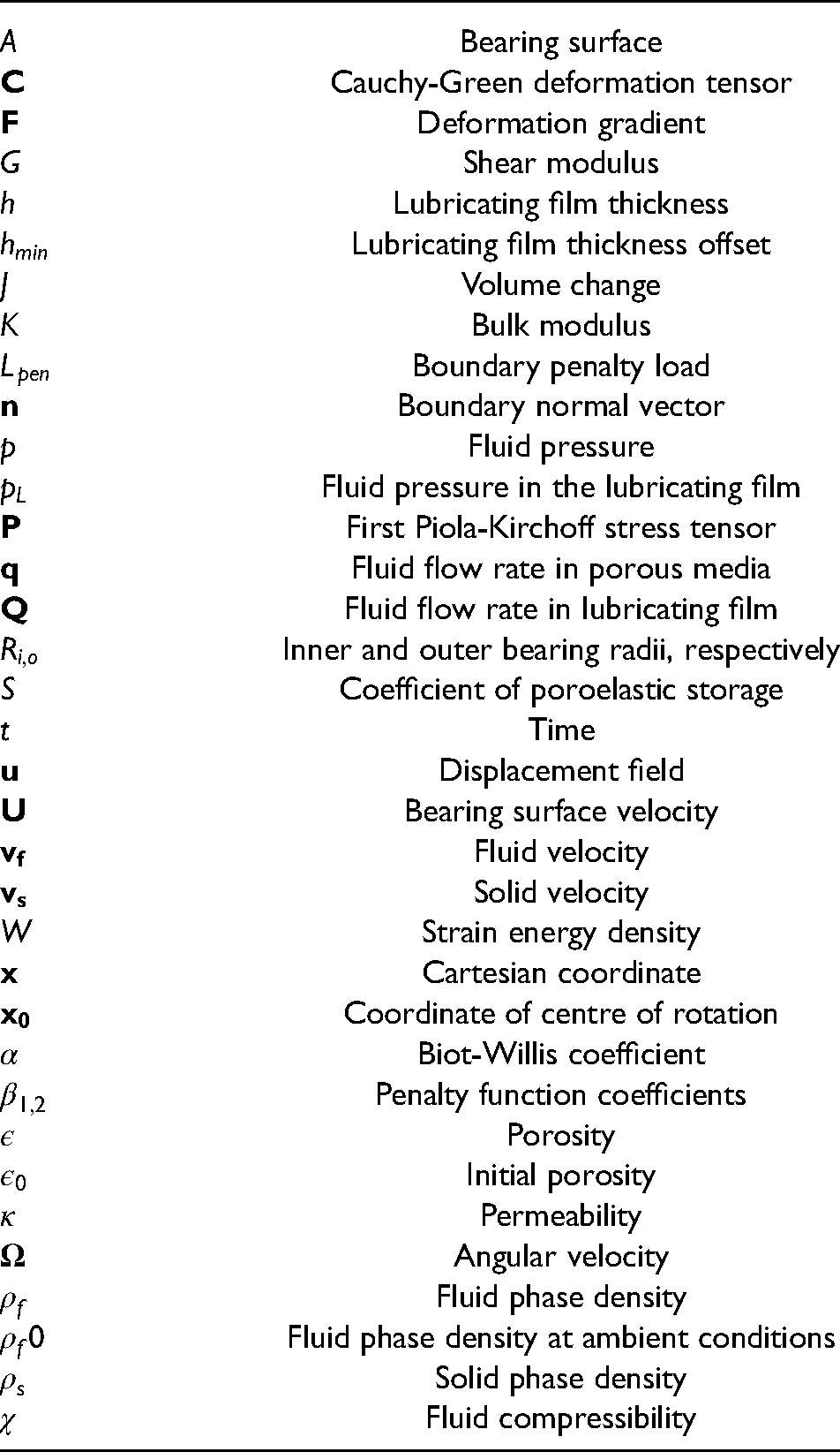
Nomenclature

Table 2.

List of nomenclature

$A$	Bearing surface
$\mathbf{C}$	Cauchy-Green deformation tensor
$\mathbf{F}$	Deformation gradient
$G$	Shear modulus
$h$	Lubricating film thickness
$h_{min}$	Lubricating film thickness offset
$J$	Volume change
$K$	Bulk modulus
$L_{pen}$	Boundary penalty load
$\mathbf{n}$	Boundary normal vector
$p$	Fluid pressure
$p_L$	Fluid pressure in the lubricating film
$\mathbf{P}$	First Piola-Kirchoff stress tensor
$\mathbf{q}$	Fluid flow rate in porous media
$\mathbf{Q}$	Fluid flow rate in lubricating film
$R_{i,o}$	Inner and outer bearing radii, respectively
$S$	Coefficient of poroelastic storage
$t$	Time
$\mathbf{u}$	Displacement field
$\mathbf{U}$	Bearing surface velocity
${\mathbf{v}}_{\mathbf{f}}$	Fluid velocity
${\mathbf{v}}_{\mathbf{s}}$	Solid velocity
$W$	Strain energy density
$\mathbf{x}$	Cartesian coordinate
${\mathbf{x}}_{\mathbf{0}}$	Coordinate of centre of rotation
$\alpha$	Biot-Willis coefficient
${\beta }_{1,2}$	Penalty function coefficients
$ϵ$	Porosity
${ϵ}_0$	Initial porosity
$\kappa$	Permeability
$\mathbf{\Omega }$	Angular velocity
${\rho }_f$	Fluid phase density
${\rho }_{f}0$	Fluid phase density at ambient conditions
${\rho }_s$	Solid phase density
$\chi$	Fluid compressibility