Sage Journals: Discover world-class research

Abstract

The application of the spectral representation method in generating Gaussian and non-Gaussian fractal rough surfaces is studied in this work. The characteristics of fractal rough surfaces simulated by the spectral representation method and the conventional Fast Fourier transform filtering method are compared. Furthermore, the fractal rough surfaces simulated by these two methods are compared in the simulation of contact and lubrication problems. Next, the influence of low and high cutoff frequencies on the normality of the simulated Gaussian fractal rough surfaces is investigated with roll-off power spectral density and single power-law power spectral density. Finally, a simple approximation method to generate non-Gaussian fractal rough surfaces is proposed by combining the spectral representation method and the Johnson translator system. Based on the simulation results, the current work gives recommendations on using the spectral representation method and the Fast Fourier transform filtering method to generate fractal surfaces and suggestions on selecting the low cutoff frequency of the power-law power spectral density. Furthermore, the results show that the proposed approximation method can be a choice to generate non-Gaussian fractal surfaces when the accuracy requirements are not high. The MATLAB codes for generating Gaussian and non-Gaussian fractal rough surfaces are provided.

Keywords

Fractal rough surface generation cutoff frequency non-Gaussian spectral representation method

Introduction

Many rough surfaces are nearly self-affine fractal within a wide range of scales, such as road surfaces, surfaces produced by fracture, and sandblasted surfaces.¹ A self-affine fractal surface looks the same when part of the surface is magnified. Moreover, the roughness parameters of self-affine fractal surfaces, such as the root-mean-square roughness and average surface curvature, are related to the measurement length scale.^2–5 Most of the widely used roughness parameters are determined based on a discrete surface height data set with a specific measurement length scale,^6,7 making it impossible to use these parameters to characterize the self-affine fractal surfaces across scales. Therefore, a scale-invariant parameter, the fractal dimension D, becomes the key to characterize roughness across scales. For a self-affine fractal surface, the fractal dimension D can be obtained through its power spectral density (PSD), which follows a power-law relationship shown in the following.

S (q) \sim q^{- 2 (H + 1)}

(1)

where S(q) represents the PSD, q is the angular frequency, and H is the Hurst exponent, related to D through H = 3 − D.⁸ In realistic surfaces, the value of q is between the low and high cutoff frequencies.

As the power-law PSD characterizes a self-affine fractal surface across scales, it has been widely used to model interfacial phenomena considering multiscale roughness, for example, contact, friction, and adhesion. These phenomena play an essential role in engineering systems, such as micro-electro-mechanical systems (MEMS), biomechanics, bearings, gears, and sealings. In these systems, the dry contact (without lubricant) between rough surfaces is one of the key factors in analyzing their performance. Many efforts have been put into the study of contact between self-affine fractal surfaces.^9–13 In addition to the dry contacts, some researchers studied lubricated contacts with fractal surfaces, for example, Li and Yang¹⁴ studied the influence of fractal surfaces on elastohydrodynamic lubrication (EHL) and Zhang et al.¹⁵ studied a thrust bearing in a mixed lubrication regime with fractal surfaces.

Most of the models mentioned above require fractal surfaces realized at specific frequency ranges. Compared with surface measurement, numerical simulation has been a popular way to obtain rough surfaces due to its convenience and economy. A large number of papers have been published about the simulation of rough surfaces.¹⁶ It should be noted that simulated rough surfaces only represent surface features within one specific evaluation area. If the evaluation area changes, the parameters used to simulate rough surfaces should be changed accordingly. At the very beginning, the mainstream in rough surface simulation is to generate surfaces with exponential PSD, which is non-fractal. There are two widely accepted conventional methods: the moving average (MA) time series model and the spectral representation method (SRM). The MA model can be implemented by different algorithms.^17–20 One of them, widely used, is the two-dimensional (2-D) digital filter method developed by Hu and Tonder,¹⁸ generating surfaces with Gaussian or non-Gaussian height distributions. The SRM was first used by Newland²¹ and Wu²² to simulate Gaussian rough surfaces. The difficulties of using the SRM to simulate non-Gaussian surfaces were studied by Wu,²³ then Wang et al.²⁴ Through these efforts, the SRM can be used in simulating non-Gaussian surfaces. Wu²² and Wang et al.²⁴ pointed that SRM has better performance in generating rough surfaces than the 2-D digital filter method. When generating non-Gaussian surfaces, the Johnson translator system is usually used in the 2-D digital filter method or the SRM. The Johnson translator system provides a group of transformation curves, which translate Gaussian random series to non-Gaussian series, and vice versa.²⁵

In terms of generating fractal surfaces, they were first studied in simulating fractal images by Voss^26,27 and Saupe²⁸ in the 1980s. They proposed several methods, including the fast Fourier transform (FFT) filtering method, random midpoint displacement (RMD), successive random additions, and Weierstrass–Mandelbrot (W–M) random fractal function. Others inherited these methods to simulate fractal rough surfaces. Majumdar and Tien⁴ first utilized the W–M fractal function method, whose PSD approximately follows the power law, to characterize and simulate the fractal roughness. Li and Yang¹⁴ also used the W–M fractal function method. Ganti and Bhushan⁵ first utilized the FFT filtering method to simulate fractal surfaces. Wu²⁹ compared the W–M fractal function method, FFT filtering method, and successive random addition method in generating fractal surfaces. It turned out that the FFT filtering method reproduces the power-law PSD better than the other two methods. Müser et al.,⁹ Borri and Paggi,³⁰ and Zhang et al.¹⁵ used the FFT filtering method as well. Besides the FFT filtering method and the W–M function, the RMD is another common choice in studies, for example, Pei et al.,³¹ Bonari et al.,³² and Vakis et al.³³ simulated fractal surfaces by the RMD for contact analysis. In addition to the methods above, Papangelo et al.¹³ and Putignano et al.³⁴ developed a spectral method, which is similar to the FFT filtering method, for simulating fractal surfaces.

The methods above are the current mainstream approaches for generating fractal surfaces. One point worthy of attention is that all these methods generate fractal surfaces with Gaussian height distribution. Only a few researchers^35,36 studied the generation of fractal surfaces with non-Gaussian height distribution. Another surprising observation is the lack of mutual learning between the simulation of fractal and non-fractal surfaces, considering the only difference between them is the expression of PSD. It seems that the development of fractal and non-fractal surface simulations are primarily independent of each other. One exception found in the literature is that Yastrebov et al.¹² used the 2-D digital filter method¹⁸ to simulate the Gaussian fractal surfaces. Furthermore, Yastrebov et al.¹² and several researchers^37,38 reported the influence of the PSD cutoff frequencies on the simulated fractal surfaces and corresponding contact simulations. However, such phenomena are ignored by most mainstream methods of simulating fractal surfaces.

Based on the literature above, although the methods for generating fractal surfaces have succeeded in many applications, they still have two shortcomings that cannot be ignored. The first is the lack of methods for non-Gaussian fractal surfaces simulation, and the other is the lack of attention in choosing the cutoff frequencies of the power-law PSD. This paper seeks to make some progress in overcoming these two shortcomings.

Inspired by the well-proven methods for simulating non-Gaussian surfaces with exponential PSD, a possible solution for simulating non-Gaussian fractal surfaces is using power-law PSD instead of the exponential PSD in those methods. Bearing this idea in mind, we noticed the high similarity between the SRM and the FFT filtering method. They have almost the same theoretical fundamentals and equations (detailed comparisons are shown in section FFT filtering method and SRM). Moreover, both have been proven to be efficient and accurate in the literature. Therefore, to generate non-Gaussian fractal surfaces, we first compare the performance of the SRM and the FFT filtering method in detail, then study the simulation of non-Gaussian fractal surfaces. In the meantime, the influence of cutoff frequencies of the power-law PSD on the simulated fractal surfaces is studied.

In summary, the current study is organized as follows. The FFT filtering method and the SRM are first compared theoretically. Then, the influences of using these two methods on the characteristics of simulated fractal rough surfaces are compared. Furthermore, the simulated surfaces are used to predict the performance of contact of rough surfaces and EHL. The differences resulting from these two simulation methods are highlighted. Next, the influence of low and high cutoff frequencies of the PSD on the simulated fractal surfaces is clarified. Finally, simulating non-Gaussian fractal surfaces are studied, and a simple approximation method is proposed.

FFT filtering method and SRM

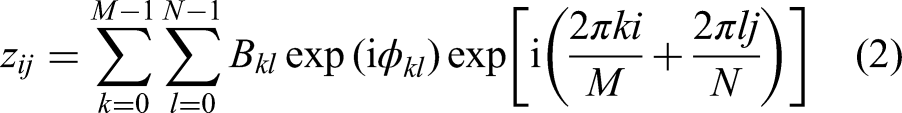
Theoretically, the FFT filtering method^5,26–30 and the SRM^21,22,39 have the same aim: generating random series with the desired PSD. They construct complex Fourier coefficients, where the amplitude terms follow the desired PSD. For the phase terms, they use random phase values following the same distribution when simulating Gaussian surfaces. Then, a sample of the random surfaces is obtained by applying the inverse Fourier transform to the Fourier coefficients constructed. Therefore, the equations of the FFT filtering method and the SRM have the same form, which is shown as equation (2):

z_{i j} = \sum_{k = 0}^{M - 1} \sum_{l = 0}^{N - 1} B_{k l} \exp (i ϕ_{k l}) \exp [i (\frac{2 π k i}{M} + \frac{2 π l j}{N})]

(2)

where,

i = 0, 1, 2, \dots, M - 1

j = 0, 1, 2, \dots, N - 1

In equation (2), the generated surface has a mesh of M × N, z_ij is the surface height at the point (i, j), B_kl is the amplitude related to the PSD value at the point (k, l), and ϕ_kl represents the random phase at the point (k, l). All ϕ_kl values are distributed uniformly over the interval [0, 2π] when simulating surfaces with the Gaussian height distribution. Equation (2) can be efficiently calculated by the FFT algorithm. One thing to note is that some restrictions in calculating B_kl and ϕ_kl are a prerequisite for using the FFT algorithm (see Appendix A).

The differences between the FFT filtering and SRM result from the calculation of the coefficient B_kl. In the SRM, B_kl is calculated as follows,^21,22,39

B_{k l} = (S_{k l})^{1 / 2}

(3)

where S_kl represents the PSD values. However, in the FFT filtering method, the equation for B_kl is^5,26–30

B_{k l} = α_{k l} (S_{k l})^{1 / 2}

(4)

where α_kl is a random number following uniform distribution over the interval [0, 1].

Based on the expressions of equations (3) and (4), it can be inferred that equation (4) results in the generated surfaces having the target PSD in average, but equation (3) can generate surfaces whose PSD is identical to the required one without considering the numerical calculation errors. In other words, the use of equation (4) makes the FFT filtering method introduce one more source of uncertainties in the simulated surfaces compared with the SRM. It should be noted that both methods have a common source of uncertainties, which is the random phase ϕ_kl.

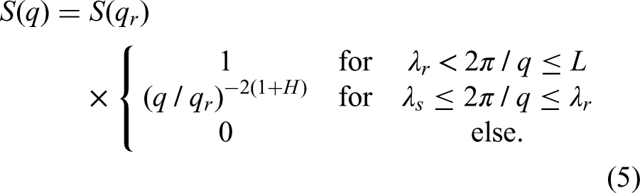
The power-law PSD used to generate fractal rough surfaces is referred to by Müser et al.,⁹ which is

S (q) = S (q_{r}) \times \{\begin{matrix} 1 & for & λ_{r} < 2 π / q \leq L \\ {(q / q_{r})}^{- 2 (1 + H)} & for & λ_{s} \leq 2 π / q \leq λ_{r} \\ 0 & else . \end{matrix}

(5)

Here, q is the magnitude of the angular frequency vector q = (q_x,q_y), and L is the linear dimension in the x and y directions, equalling 0.1 mm. q_r = 2π/λ_r is the roll-off angular frequency, λ_r = 20 µm is the corresponding roll-off wavelength, and λ_s = 0.1 µm sets the short-wavelength cutoff. H is the Hurst roughness exponent, which equals 0.8. S(q_r) denotes the PSD amplitude and is related to the variance (σ²) of the simulated surfaces. The root-mean-square roughness (standard deviation (SD) σ) of the simulated surfaces is 0.762 µm.

Simulation of non-Gaussian rough surfaces

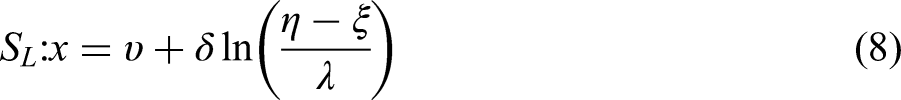
Many conventional and widely used methods of simulating non-Gaussian rough surfaces^{18–20,24,40} are based on the Johnson translator system.²⁵ The Johnson translator system includes three types of transformation curves, which are as follows.

S_{U} : x = υ + δ \sinh^{- 1} (\frac{η - ξ}{λ})

(6)

S_{B} : x = υ + δ \ln (\frac{η - ξ}{ξ + λ - η})

(7)

S_{L} : x = υ + δ \ln (\frac{η - ξ}{λ})

(8)

where x denotes the Gaussian series, η is the non-Gaussian series, and ν, δ, ξ, λ are the parameters derived by Hill’s algorithm⁴¹ by the first four moments of η. The first four moments of a random series are mean (μ), variance (σ²), skewness (Ssk), and kurtosis (Sku). Francisco and Brunetiere⁴² pointed out that the conventional Johnson translator system cannot generate highly accurate random series with specific skewness and kurtosis values. They provided a rather complicated hybrid method for simulating non-Gaussian surfaces. Nevertheless, the Johnson translator system is used in this study as it is easy to use and widely accepted.

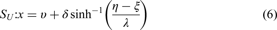
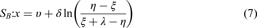
While transferring the Gaussian series to the non-Gaussian series, the PSD will be distorted. Such distortion of PSD needs to be corrected before it is used to simulate non-Gaussian surfaces. To tackle this problem, Wang et al.²⁴ used an iteration method to approximate the desired PSD, which is compatible with the translation from the Gaussian to the non-Gaussian series. The method of Wang et al.²⁴ first fits the Johnson translator system by the target Ssk and Sku values and provides a translation process that translates the Gaussian series to the target non-Gaussian series. Based on the relationship between the autocorrelation function (ACFs) before and after the translation, an underlying PSD compatible with the non-Gaussian height distribution is iteratively approximated. Next, with this underlying PSD, a Gaussian rough surface can be simulated by the SRM. Finally, the simulated Gaussian surface is translated to the required non-Gaussian surface by the fitted Johnson curve. This non-Gaussian surface should have both the required PSD and target Ssk and Sku with high accuracy. The detailed procedures of this method can be found in the work of Wang et al.²⁴ In the current study, this method is tested with the power-law PSD.

Results and discussion

Surfaces generated by the FFT filtering method and SRM

Gaussian fractal rough surfaces with a grid size of 2048 × 2048 were generated by the FFT filtering method and SRM. As the FFT filtering method has two sources of uncertainties (amplitude and phase terms in equation (2)), while the SRM has one (phase term in equation (2)), the generation of random samples of these two methods is different in the current study.

For the FFT filtering method, the random samples were selected by following rules to highlight the influence of uncertainties caused by the amplitude term. For each set of fixed phase term ϕ_kl values, 1000 fractal surfaces were generated with altering B_kl values by equation (4). Furthermore, to show the influence of the two uncertainty sources preliminarily, 100 different sets of phase term values were used. For the SRM, as the phase term is the only uncertainty source in equation (2), 1000 fractal surfaces were simulated with altering ϕ_kl values, while the B_kl values were the same as calculated by equation (3).

Figure 1 shows the central line profiles, which is the 1024th row of the simulated surfaces. The surfaces used to plot this figure were simulated with the same ϕ_kl values. Therefore, the central line profile of the surface simulated by the SRM is a single line, while the FFT filtering method provides 1000 central line profiles. The mean profile of these 1000 profiles was plotted, and their SD was also plotted to show the uncertainties. Figure 1 clearly shows that the mean central line profile of surfaces simulated by the FFT filtering method agrees well with the single profile generated by the SRM. The SD corresponding to the profiles resulted from the FFT filtering method has a magnitude of 0.3 μm.

Figure 1.

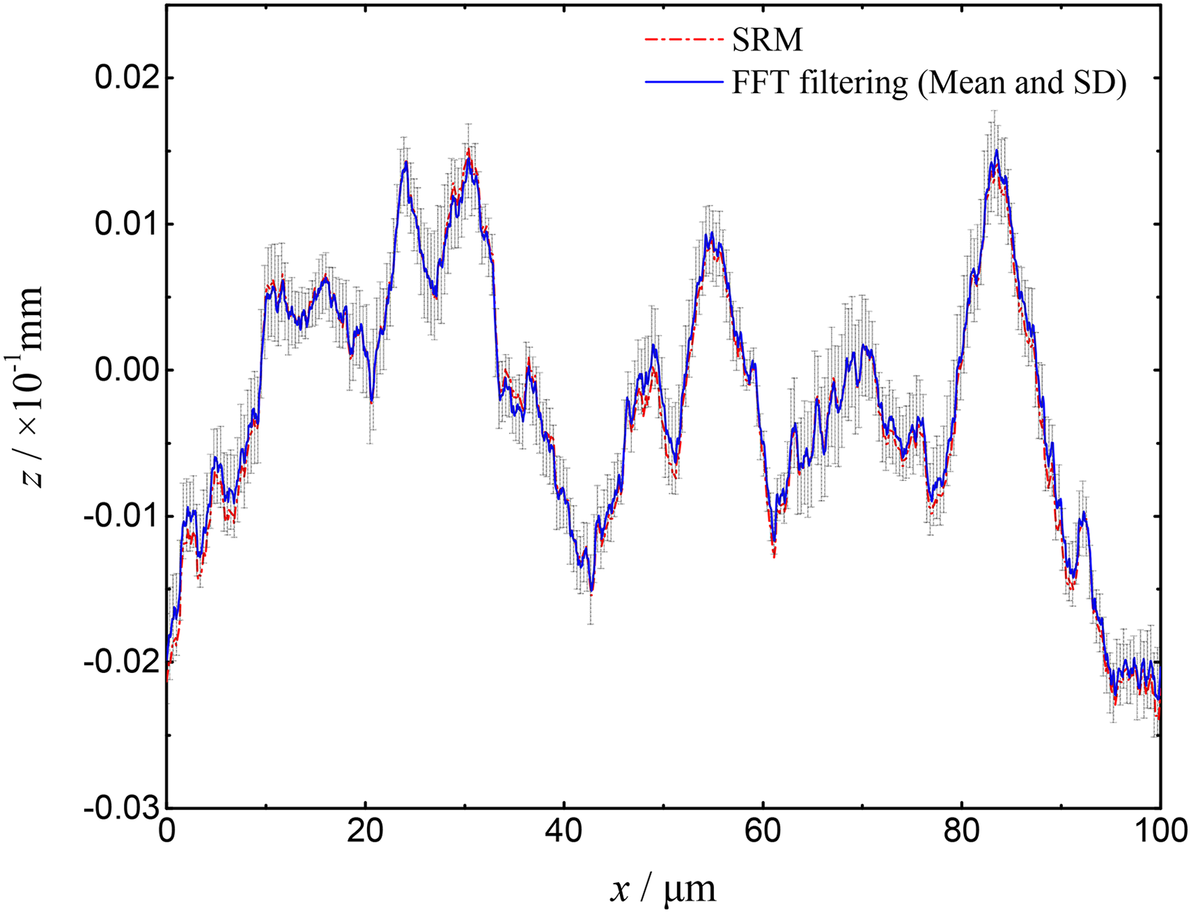
Central line profiles of fractal surfaces simulated by the FFT filtering method and SRM.

Figure 2 shows the target PSD, mean PSD of the surfaces simulated by the SRM, and the mean PSD of the surfaces simulated by the FFT filtering method. Again, the SD values were taken to illustrate the uncertainties. It clearly shows that the mean PSD of the surfaces simulated by the SRM perfectly matches the target one. Furthermore, the most significant SD value is at the magnitude of 1 × 10⁻¹⁹, which is still too small to plot in Figure 2. Such a result means that every single surface generated by the SRM can reproduce the target PSD very well. In comparison, the mean PSD resulted from the FFT filtering method approximately follows the target one and has significant deviations occurring at some frequencies.

Figure 2.

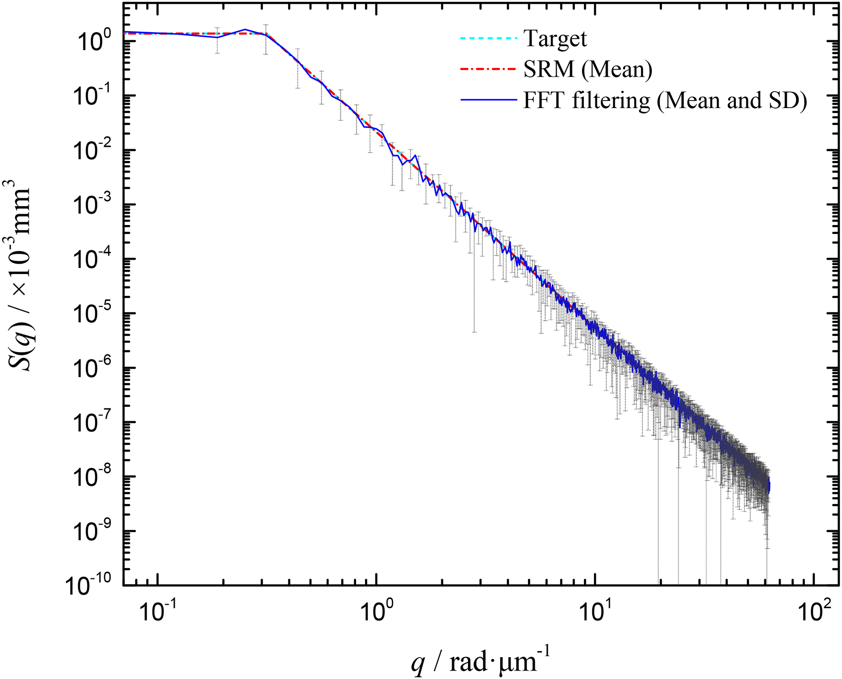
PSD of fractal surfaces simulated by the FFT filtering method and SRM.

To further characterize the simulated surfaces, several widely used roughness parameters were calculated, including the skewness (Ssk), kurtosis (Sku), root-mean-square gradient (Sdq), summit density (Sds), and mean summit radius (Rc). Ssk and Sku can help to characterize the surface height distribution. Sdq, Sds, and Rc are based on the definition of the summit of roughness. Detailed information on the calculation of these parameters is given in Appendix B. One more thing worthy of knowing about these parameters is that they are traditional statistical roughness parameters and cannot comprehensively characterize rough surfaces. Some parameters defined by morphological methods can enhance the analysis of simulated surfaces in future work.⁴³

Figure 3 shows the roughness parameters calculated based on the surfaces simulated by the FFT filtering method. The abscissa represents the 100 different groups of ϕ_kl values. For each group of ϕ_kl, the roughness parameters of the 1000 simulated surfaces with randomized B_kl values were averaged, and the corresponding SDs were plotted to show the uncertainties. It can be seen that uncertainties in the ϕ_kl and B_kl values affect the output roughness parameters. In particular, Ssk, Sku, and Sds are significantly influenced by ϕ_kl, while the Sdq and Rc are not sensitive to it. The reason should be that the phase term ϕ_kl determines the height distribution of the simulated surfaces theoretically. The Ssk and Sku are the parameters to characterize the height distribution, and the Sds is closely related to the height distribution. Thus, these three parameters are sensitive to the change of ϕ_kl. As for the Sdq and Rc, they are more relevant to the spatial information of the roughness, which is mainly dominated by the PSD in theory. Hence, they are not influenced much by changing the ϕ_kl values.

Figure 3.

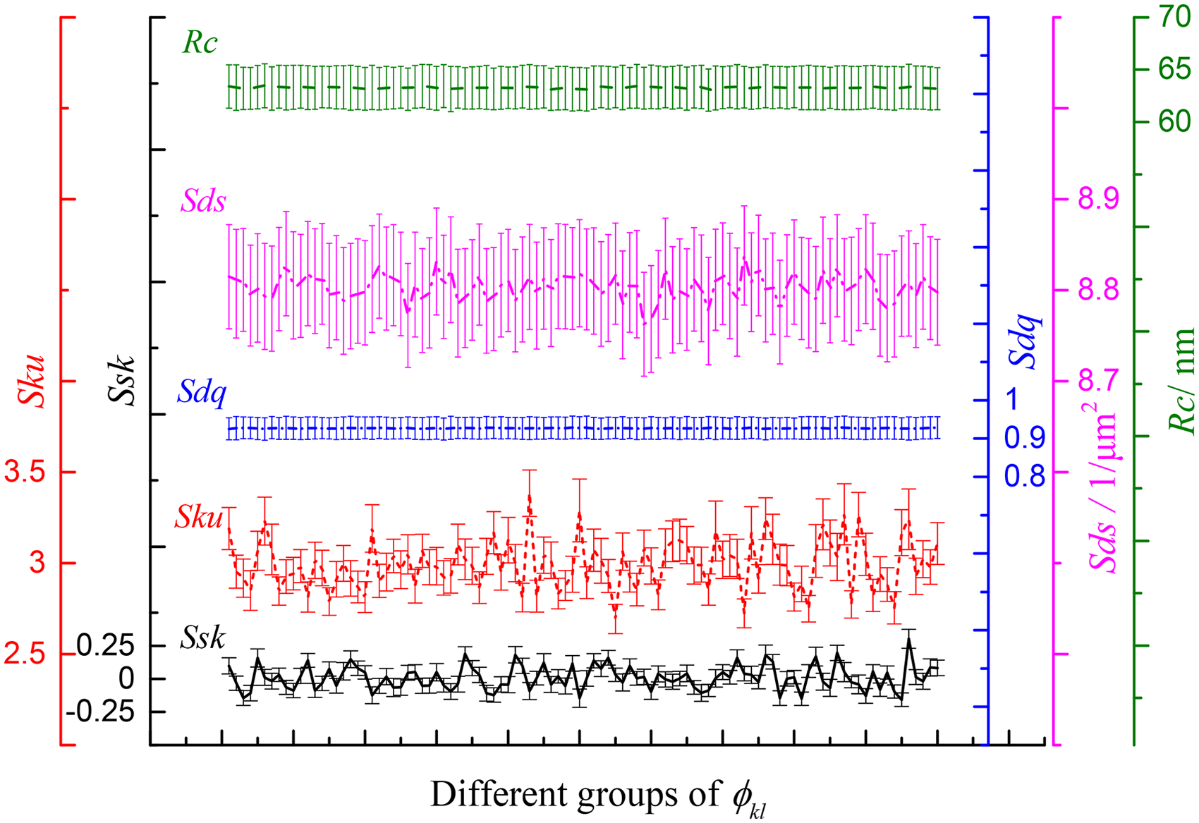
Roughness parameter values of fractal surfaces simulated by fast Fourier transform (FFT) filtering method.

Unlike the uncertainties introduced by the ϕ_kl, the uncertainties in the B_kl have significant influences on all the five roughness parameters. The magnitude of such influences on each parameter can be estimated by taking the average, and SD of the standard deviation (SD) values caused by the uncertainties in the B_kl with the 100 different groups of ϕ_kl values. The corresponding results are listed in Table 1. The mean value of the SD values is different for different roughness parameters, while the SD of the SD values is tiny for all the five roughness parameters. This result means that the uncertainties of a specific roughness parameter caused by the uncertain B_kl are at the same magnitude with different ϕ_kl values. Moreover, the two sources of uncertainties (amplitude and phase) in the FFT filtering method are probably irrelevant regarding the influences on the roughness parameters discussed in this paper.

Table 1.

Mean and standard deviation of the SD values caused by the uncertainties in the B_kl.

Parameter	Mean of SD values	The SD of SD values
Ssk	0.06	0.0063
Sku	0.10	0.0209
Sdq	0.29	0.0071
Sds/μm⁻²	0.06	0.0014
Rc/nm	2.05	0.0490

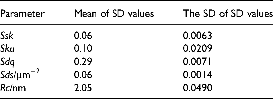
Figure 4 plots the roughness parameters calculated based on the surfaces simulated by the SRM. The abscissa represents 1000 different groups of ϕ_kl values. Once more, it shows that different sets of ϕ_kl values dramatically influence the Ssk, Sku, and Sds values but hardly affect the Sdq and Rc. The mean Ssk, Sku, and Sds values of the 1000 simulated surfaces are 0.004, 2.98, and 8.8 μm⁻², with a SD of 0.11, 0.17, and 0.025, respectively. It is expected that the mean Ssk and Sku values with different groups of ϕ_kl values approach the values of an ideal Gaussian distribution, which are 0 for the Ssk and 3 for the Sku. When the ϕ_kl is fixed (see Figure 3), only considering the uncertainties in the B_kl cannot get mean Ssk and Sku values approaching the ideal Gaussian distribution, but some values determined by the phase term used. Therefore, the uncertainties in the ϕ_kl (phase term) have a more important role in simulating Gaussian surfaces than the uncertainties in the B_kl (amplitude term). The other point worthy of notice is the comparisons between the SDs of Ssk, Sku, and Sds caused by the uncertain ϕ_kl and B_kl. For the Ssk and Sku, the SDs caused by the uncertain ϕ_kl (0.11 and 0.17) are more significant than those caused by the uncertain B_kl (0.06 and 0.10, see Table 1). For the Sds, the uncertain ϕ_kl results in a standard deviation of 0.025, less than the SD caused by the uncertain B_kl (0.06, see Table 1).

Figure 4.

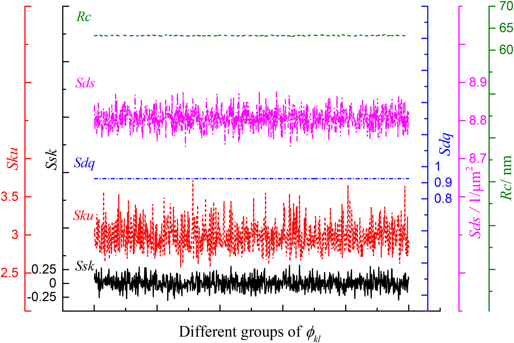
Roughness parameter values of fractal surfaces simulated by the spectral representation method (SRM).

In addition to the comparisons of roughness profiles and parameters, a more critical issue is to compare the surfaces simulated by the FFT filtering method and the SRM in tribological applications. Therefore, two classic tribological applications, contact between rough surfaces and EHL, are conducted.

Contact of rough surfaces

The parameters set for contact simulation are extracted from Müser et al.⁹ The fractal rough surfaces are pressed down to a flat rigid surface. The equivalent Young’s modulus is E* = 25 MPa. The applied load varies from 0.0001E* to 0.9E*. To highlight the influence of uncertainties in the B_kl and save computational resources, 100 surfaces simulated by the FFT filtering method, and one surface simulated by the SRM with the same ϕ_kl values were used in the contact simulation. The numerical procedures for solving these contact problems can be found in the work of Marklund et al.⁴⁴

Three parameters were calculated during the simulations: the relative contact area a_r, mean contact pressure p_c, and mean gap u_g. The relative contact area a_r is the ratio of the real contact area to the nominal contact area. The mean contact pressure p_c is the arithmetic mean of the contact pressure values at each contact node. The mean gap u_g is the mean height of the deformed rough surface. These parameters were plotted versus applied loads, respectively (Figures 5 to 7).

Figure 5.

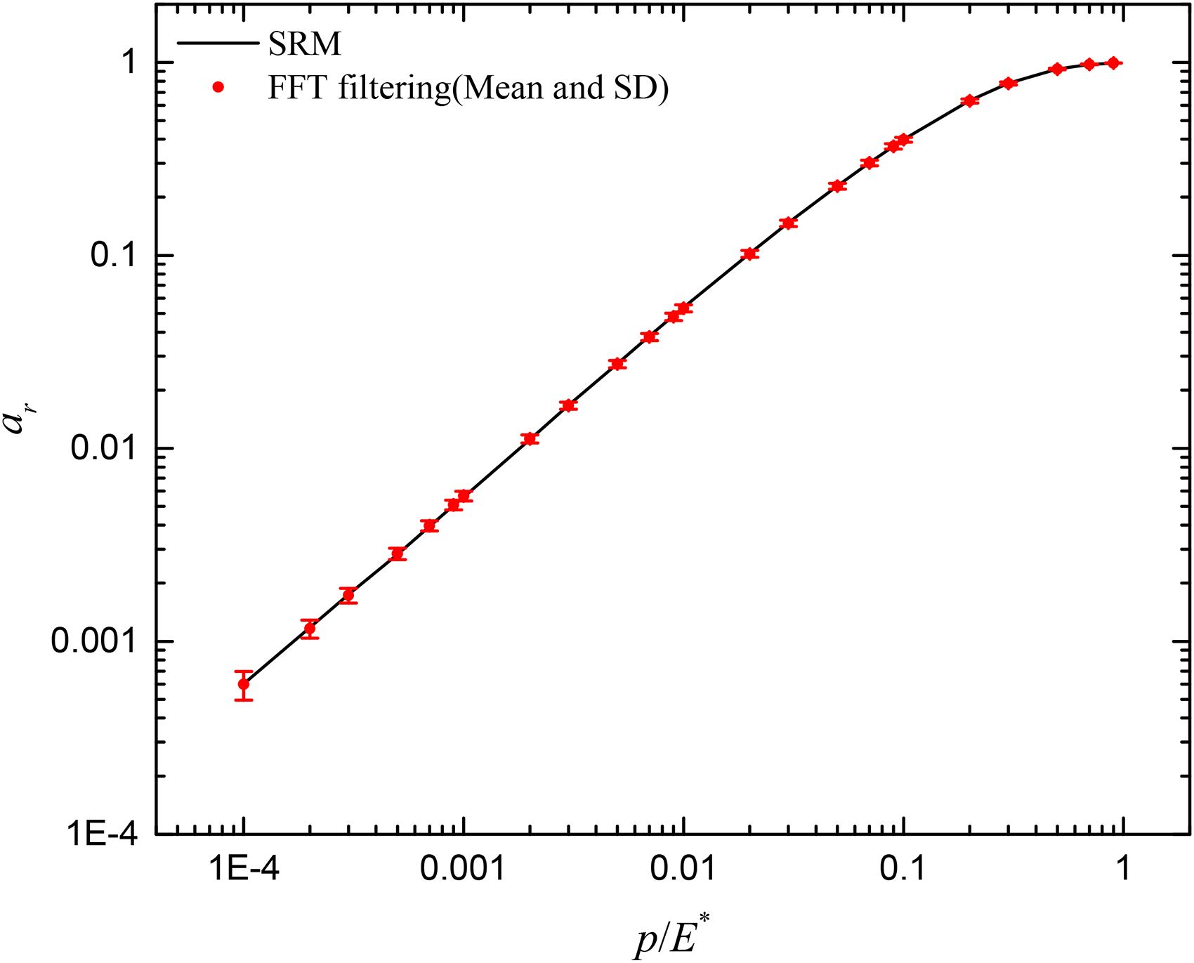
Relative area a_r values with fractal surfaces simulated by FFT filtering and SRM.

The results show that, on average, the a_r, p_c, and u_g values calculated from the contact of surfaces simulated by the FFT filtering method agree well with those using surfaces simulated by the SRM. Figure 5 shows that the relative contact area a_r values are slightly influenced by using the FFT filtering method with a wide range of applied loads, especially with smaller applied loads. Figure 6 illustrates that with smaller applied loads, the mean contact pressure p_c values are significantly influenced when the surfaces simulated by the FFT filtering method are used. With smaller applied loads, the contact spots and contact pressures are easily affected by small asperities, which results in more significant uncertainties in the a_r and p_c values. As for the mean gap, it can be seen in Figure 7 that the u_g values are sensitive to the use of the FFT filtering method with larger applied loads. This result should be because large applied loads lead to more significant interactions between asperities. Thus, the surface deformation is more sensitive to the changes in asperity distribution, resulting in more significant deviations in the u_g values. Another point worth noting from Figures 5 to 7 is that the choice of method does not affect the dry contact simulation result much. This finding allows a direct comparison between dry contact simulations that used the FFT filtering method and the SRM.

Figure 6.

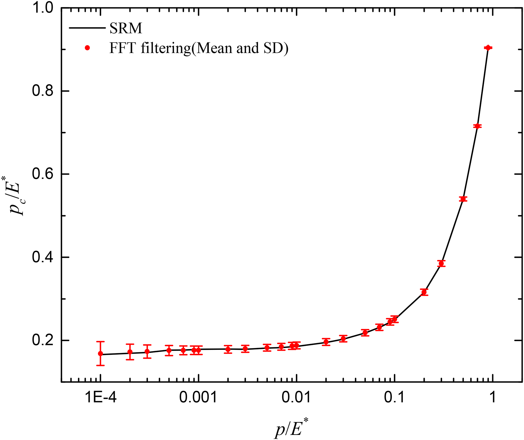
Mean contact pressure p_c values with fractal surfaces simulated by FFT filtering and SRM.

Figure 7.

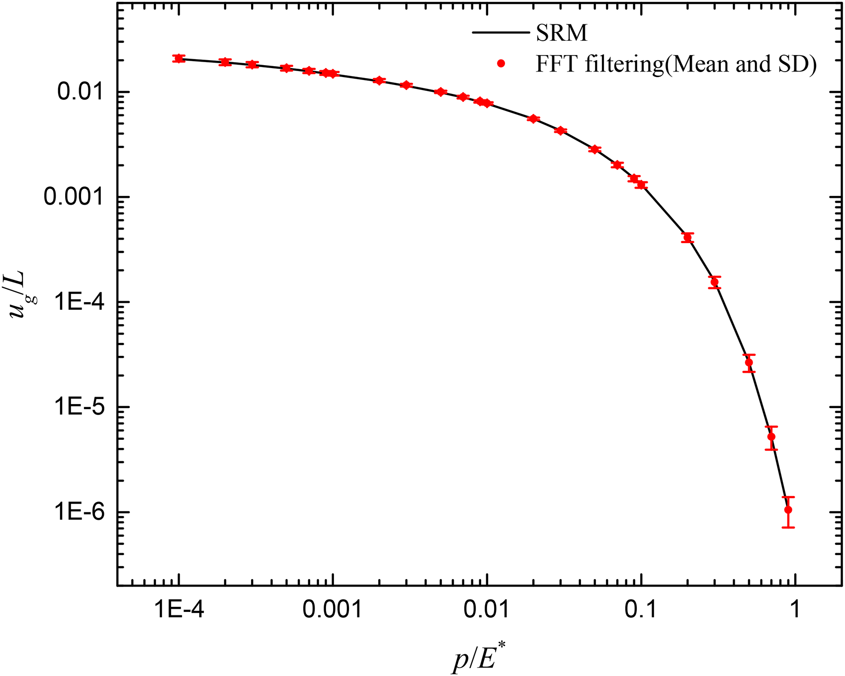
Mean gap u_g values with fractal surfaces simulated by FFT filtering and SRM.

EHL simulation

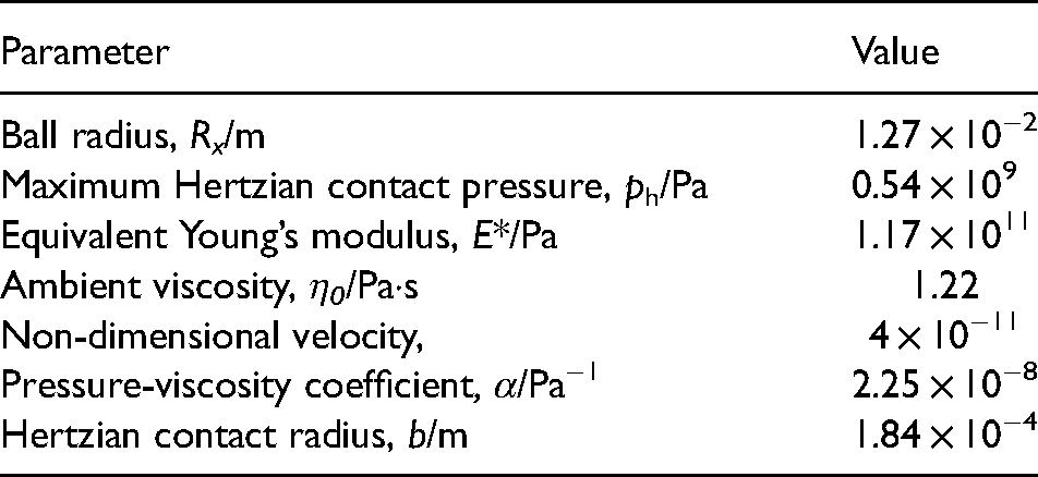
A typical point contact EHL problem defined in the work of Venner and Lubrecht⁴⁵ is used in the current work. The corresponding parameters are listed in Table 2. The transient Reynolds equation is used. Ten surfaces simulated by the FFT filtering method and one surface simulated by the SRM with the same ϕ_kl values are used to reduce the calculation amount as the transient EHL is considered. All the simulated surfaces were sampled down to the size of 256 × 256 to save computational resources further. One thing to note is that the sampling-down process is not a recommended method to generate rough surfaces for EHL simulation, and it is used here only for numerical convenience. If one wants to run some accurate EHL simulations, it is better to regenerate rough surfaces after adjusting the mesh size and cutoff frequencies. The time step was set to the value, making the surface move one mesh grid at each time step. Such a setting means that after every 257 time steps, the roughness matrix is cycled once. The total number of time steps was set to 13 times the time steps needed for one cycle of the surface, by which the transient system reaches a steady state. The root-mean-square roughness value was reduced to 0.0762 μm to avoid any asperity contacts in the Hertzian contact zone. It should also be noted that the solution domain is a square area whose side length is four times the radius of the Hertzian contact zone, which is bigger than the area of the simulated surfaces (0.1 mm × 0.1 mm). Here to simplify the simulation setup, all the simulated surfaces were assigned to the mesh of the solution domain. The simulations ran on the ARC3, part of the high-performance computing facilities at the University of Leeds, UK, with E5-2650v4 CPU, 2.2 GHz.

Table 2.

Parameters for the elastohydrodynamic lubrication (EHL) simulation.

Parameter	Value
Ball radius, R_x/m	1.27 × 10⁻²
Maximum Hertzian contact pressure, p_h/Pa	0.54 × 10⁹
Equivalent Young’s modulus, E*/Pa	1.17 × 10¹¹
Ambient viscosity, η₀/Pa·s	1.22
Non-dimensional velocity, $U = η_{0} u_{s} / (2 E^{*} R_{x})$	4 × 10⁻¹¹
Pressure-viscosity coefficient, α/Pa⁻¹	2.25 × 10⁻⁸
Hertzian contact radius, b/m	1.84 × 10⁻⁴

Based on the simulation results, the minimum film thickness h_min and maximum pressure p_max were extracted. The h_min and p_max values from the last 257 time steps were plotted in Figures 8 and 9, respectively. Figure 8 shows that the h_min resulting from the SRM-generated surface has a similar trend with the mean h_min calculated using the FFT filtering method simulated surfaces, but the specific values vary significantly. The curves in Figure 9 show the p_max results in the same manner. The mean p_max values calculated using the FFT filtering method simulated surfaces have almost the same trend as the p_max values obtained using the surface generated by the SRM. Generally, the parameters of interest calculated in the transient problem are averaged in the last complete surface cycle to represent the steady-state results. Therefore, the h_min and p_max values in the last cycle were averaged. With the surface simulated by the SRM, the averaged h_min and p_max are 0.282 μm and 2.32p_hPa, respectively. For the surfaces simulated by the FFT filtering method, the averaged h_min and p_max are 0.284 μm and 2.28p_hPa, respectively. From this perspective, the results obtained with surfaces simulated by the FFT filtering method and SRM match each other. However, compared with the results of rough surface contact, using the FFT filtering method or SRM has a more significant influence on EHL performance prediction. It is worth mentioning that each transient EHL simulation here needs around 25 h to finish. Using 10 rough surfaces generated by the FFT filtering method means around 250 h. This considerable cost can be reduced just by using the one rough surface simulated by the SRM.

Figure 8.

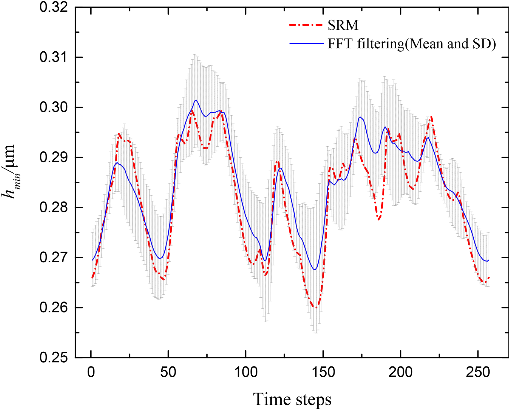
Minimum film thickness, h_min values of the last cycle of surface.

Figure 9.

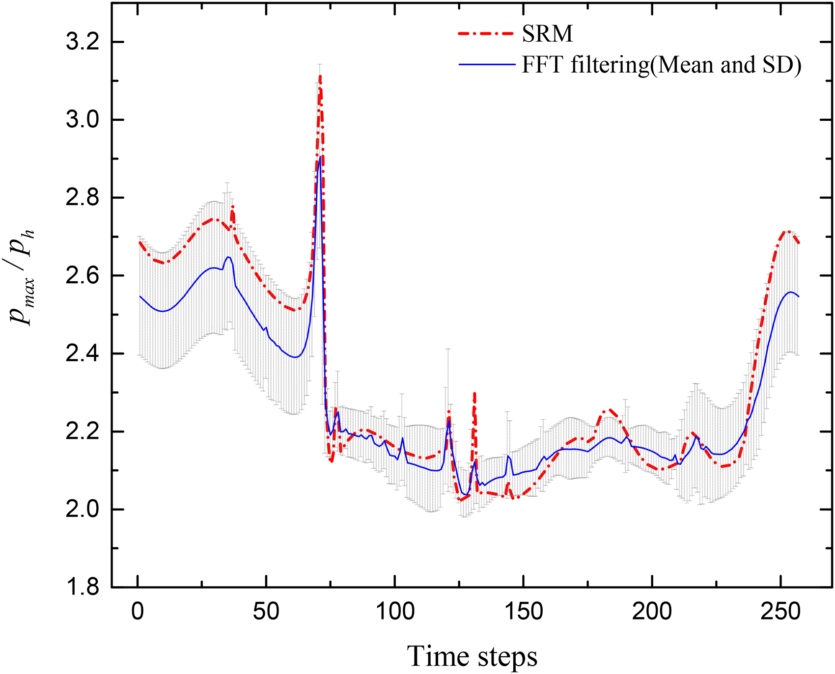
Maximum pressure, p_max values of the last cycle of surface.

In summary, the FFT filtering method introduces one more source of uncertainties, the amplitude term in equation (2), in the simulated surfaces compared with the SRM. When the phase term, the common source of uncertainties in the two methods, is fixed, the FFT filtering method generates surfaces whose mean profile approaches the unique surface generated by the SRM. Moreover, the FFT filtering method introduces uncertainties in the PSD of simulated surfaces, while the SRM can perfectly reproduce the given power-law PSD. Furthermore, through a preliminary analysis of roughness parameters, the two sources of uncertainties (amplitude and phase) in the FFT filtering method are probably irrelevant. Testing the two methods with the rough contact and EHL simulations demonstrates that one SRM simulated surface can represent the averaged results from several surfaces simulated by the FFT filtering method when the phase term is fixed. Hence, the SRM seems to be a better method to generate accurate and representative fractal rough surfaces for predicting tribological performance. However, this does not mean that using the FFT filtering method is wrong, as real measured surfaces have uncertainties in their PSDs. Considering such uncertainties or not needs comprehensive studies about their influences on tribological properties in different applications. Based on the analysis in this paper, the uncertainties in PSD do not affect scenarios where the average influence of rough surfaces is more important. Such results do not rule out that some applications in which the extreme conditions matter and the uncertainties in PSD have a significant impact, for example, fluid sealing and micropitting. Therefore, we recommend the SRM when the average influence of rough surfaces is of more concern.

The influence of low and high cutoff frequencies

To better understand the effect of cutoff frequency on the normality of simulated fractal surfaces, the PSD with and without roll-off is investigated with different low and high cutoff frequencies in this section. Moreover, the traditional non-fractal exponential PSD is used as a comparison. Based on the discussions in the section Surfaces generated by the FFT filtering method and SRM, only the SRM is used here for numerical efficiency.

According to previous work considering the cutoff frequencies in simulating fractal surfaces,^12,37,38 the ratios of low (high) cutoff frequency to the lower bound (upper bound) of the frequency range of the surface are essential parameters affecting the normality of simulated surfaces. In the current work, the ratio of low cutoff frequency, q_l, to the lower bound of the surface frequency range, q_min, was set as q_l/q_min = 1, 1.4, 2.5, 5, and 10. The ratio of high cutoff frequency, q_s, to the upper bound of the surface frequency range, q_max, was set as q_s/q_max = 0.1, 0.14, 0.24, 0.5, and 1. While altering the q_l/q_min values, the q_s/q_max was fixed at 1. When the different q_s/q_max values were used, the q_l/q_min was set at one. Furthermore, for roll-off PSD, the roll-off wavelength in equation (5), λ_r was fixed at 20 μm, while for single power-law PSD, λ_r equaled 100 μm to remove the plateau region in PSD shown in equation (5).

For each different cutoff frequency value, 1000 surfaces were generated with different ϕ_kl values. Furthermore, all the simulated surfaces were normalized to zero mean and unit standard deviation. To quantitatively evaluate the normality of the simulated surfaces, the histogram of the simulated surface was calculated and compared with the standard Gaussian distribution histogram. Furthermore, the differences between the histogram of simulated surfaces and the standard Gaussian distribution were calculated as errors referring to Pérez-Ràfols and Almqvist.³⁶ The histogram of a set of random data is calculated by dividing the range of the data set into intervals covering the lowest to the highest value of the data set. Such intervals are referred to as bins. The frequency, n_i is the number of heights falling in the specific interval over the total number of data points. The number of bins is chosen based on Scott’s rule, which is automatically implemented by MATLAB. The histograms of simulated surfaces and standard Gaussian distribution used the same bins. Therefore, the error of histogram, e_h is calculated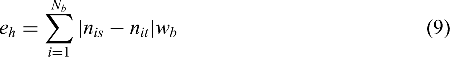

e_{h} = \sum_{i = 1}^{N_{b}} | n_{i s} - n_{i t} | w_{b}

(9)

where n_is is the frequency of histogram of simulated surfaces, n_it is the frequency of standard Gaussian distribution, w_b is the width of bins, and N_b is the number of bins.

First of all, the influence of low cutoff frequency is analyzed. Figure 10 shows the mean histogram of simulated surfaces with roll-off PSD and the corresponding standard deviation for q_l/q_min = 1. The standard Gaussian histogram was also plotted as a reference. The mean histogram of simulated surfaces matches well with the standard Gaussian, showing good normality. However, the corresponding SD shows that each simulated surface histogram could significantly deviate standard Gaussian, especially near the surface mean height. The mean e_h of simulated surface histograms is 5.04 × 10⁻², quantifying the degree of such deviation. In Figure 11, the histograms of simulated surfaces with single power-law PSD were plotted for q_l/q_min = 1. The results clearly show that even the mean histogram of simulated surfaces has significant discrepancies with the standard Gaussian. The corresponding standard deviation values are much larger than those shown in Figure 10, resulting in a larger mean e_h = 2.24 × 10⁻¹. Figure 12 shows the histogram when q_l/q_min = 10, by which the q_l is greater than the roll-off frequency q_r, means that the PSD with or without roll-off gives the same pattern. Thus, the histograms shown in Figure 12 represent the results for q_l/q_min = 10 whether the PSD with roll-off or not. In Figure 12, it is readily seen that the mean histogram of simulated surfaces has a better agreement with the standard Gaussian, and the corresponding SD values are smaller than those in Figures 10 and 11, providing a mean e_h as small as 1.85 × 10⁻².

Figure 10.

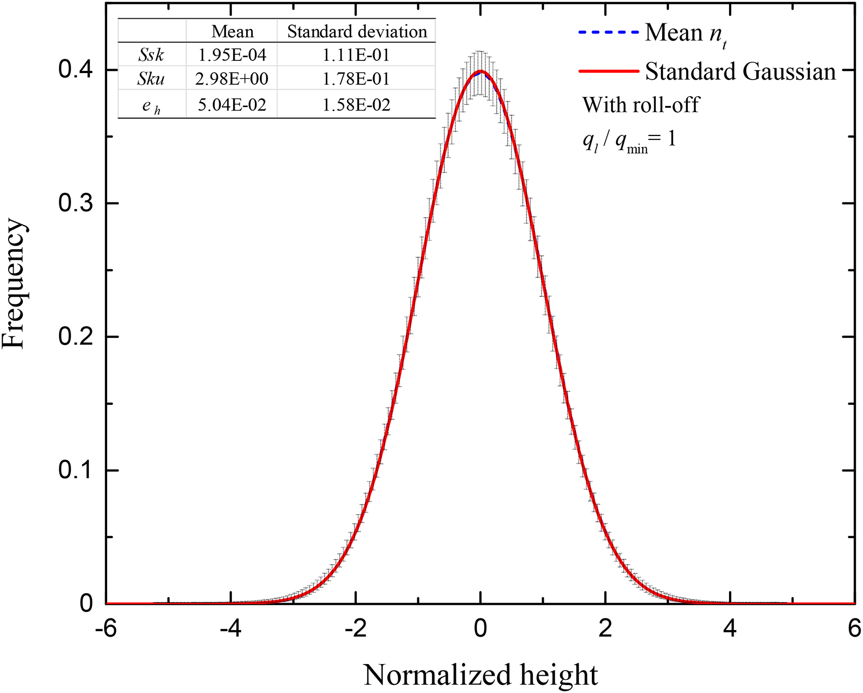
Mean histogram of simulated surfaces and corresponding standard deviation with roll-off power spectral density (PSD), q_l/q_min = 1.

Figure 11.

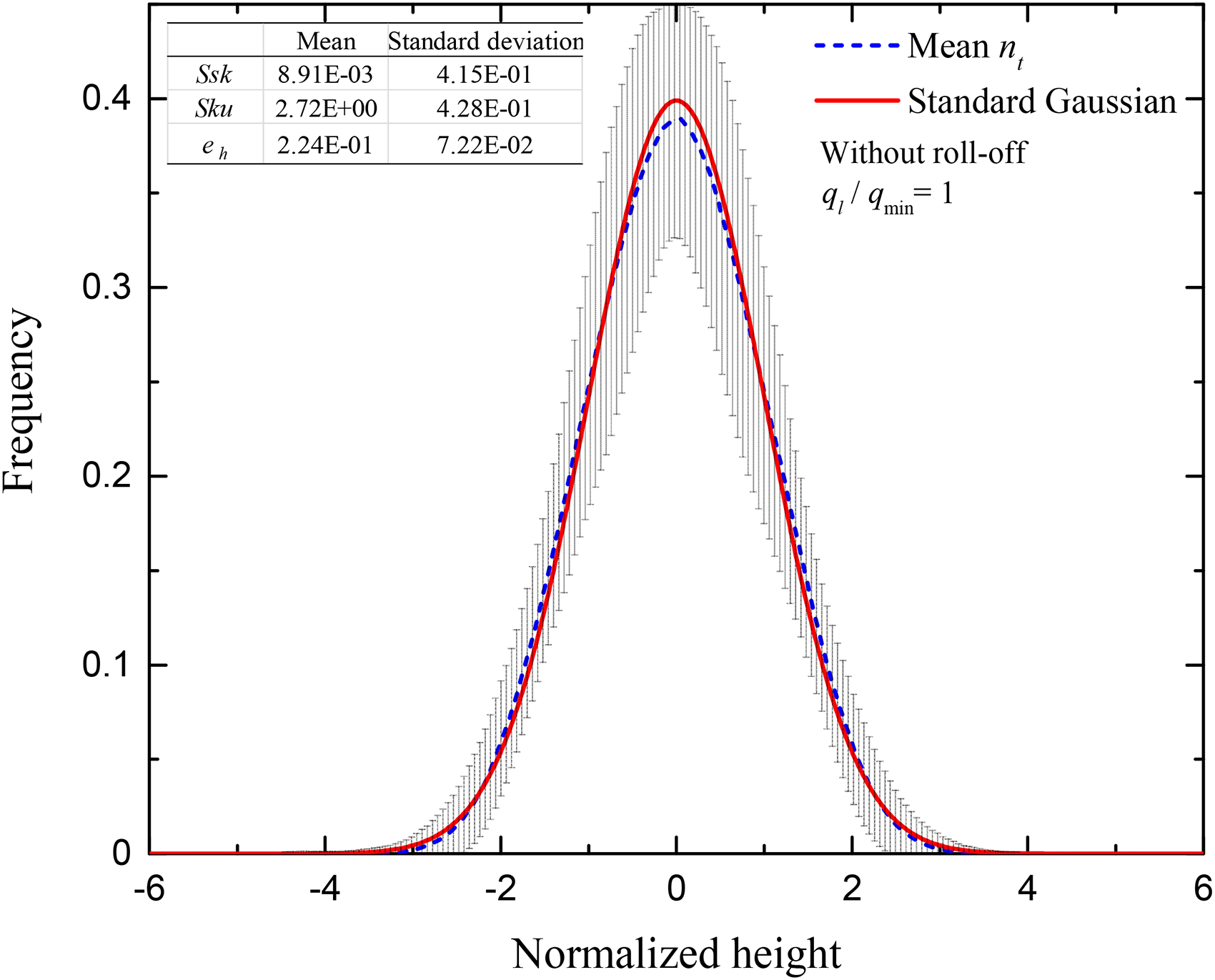
Mean histogram of simulated surfaces and corresponding standard deviation with single power-law power spectral density (PSD), q_l/q_min = 1.

Figure 12.

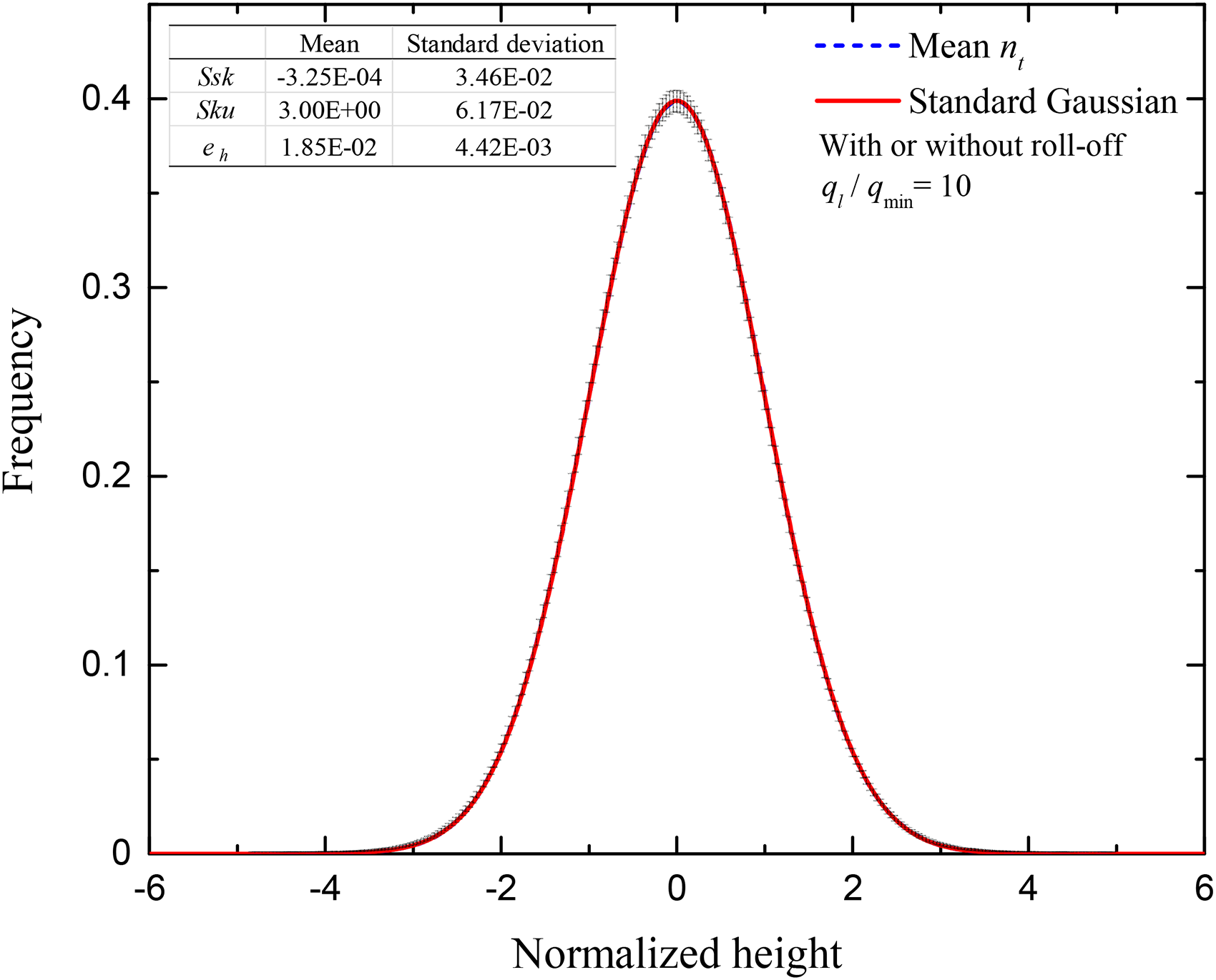
Mean histogram of simulated surfaces and corresponding standard deviation with or without power spectral density (PSD) roll-off, q_l/q_min = 10.

Furthermore, Figure 13 shows the mean e_h values and corresponding SD values with different q_l/q_min values. As the q_l/q_min increases, the mean e_h decreases, and the corresponding SD also decreases. Also, roll-off PSD dramatically reduces the mean e_h values and SDs when the q_l/q_min value is close to 1. These results mean that, first, a large q_l/q_min value, for example, >5, can sufficiently improve the normality of each simulated surface, as the mean e_h values and their SDs are reduced simultaneously. Second, with the PSD showing a plateau region, meaning roll-off frequency is larger than the low cutoff frequency, the q_l/q_min value has a much weaker effect on the normality of the simulated surfaces. Therefore, if inevitable, for PSD with a plateau region, q_l/q_min value could equal 1 to generate Gaussian fractal surfaces having acceptable normality. However, for the single power-law PSD, the q_l/q_min value shall be at least >1, which is also suggested by Yastrebov et al.¹²

Figure 13.

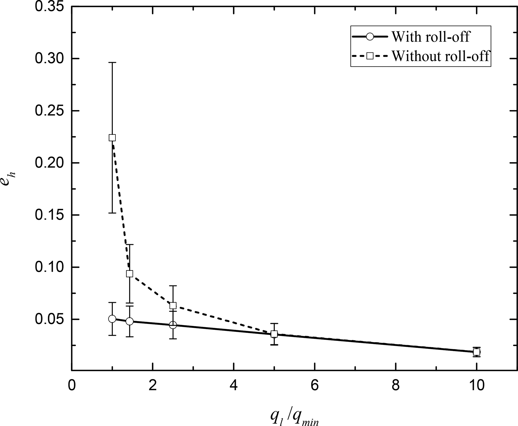
Mean histogram error e_h and corresponding standard deviation for different q_l/q_min values.

Next, the different q_s/q_max values were used to simulate surfaces. Figure 14 shows the mean e_h values and corresponding SD values with various q_s/q_max values for PSD with and without the plateau region. The results prove that the q_s/q_max does not affect the normality of simulated surfaces whether the PSD has a plateau region or not.

Figure 14.

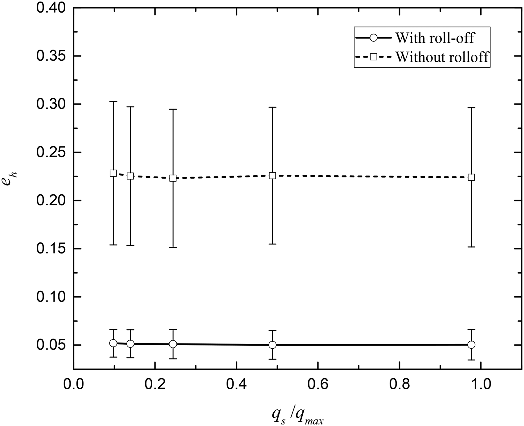
Mean histogram error e_h and corresponding standard deviation for different q_s/q_max values.

In comparison, the exponential PSD for the simulation of non-fractal surfaces was tested. The exponential PSD was calculated by the Fourier transform of the exponential ACF, which is defined by $R (p, q) = \exp [\log (0.1) \sqrt{{(p / 30)}^{2} + {(q / 30)}^{2}}]$ . The q_l/q_min and q_s/q_max both equal 1. Figure 15 plots the mean histogram and corresponding SD of simulated surfaces with exponential PSD. It clearly shows that the mean histogram of simulated surfaces matches the standard Gaussian with a tiny SD. Comparing Figure 15 with Figure 12, the magnitude of the SD in Figure 15 is much smaller than that in Figure 12. Such phenomenon is reflected by the e_h value as well. For Figure 15, the mean e_h value is 9.61 × 10⁻³, which is smaller than 1.85 × 10⁻² in Figure 12. It is worth mentioning that the q_l/q_min value equals 1 for the results in Figure 15 but equals 10 for those in Figure 12. These results mean one can ignore the influence of q_l/q_min when the target PSD is exponential. Therefore, it seems that the significant influence of q_l/q_min on the normality of simulated surfaces is a particular case resulted from the power-law PSD and only needs to be considered for the simulation of fractal surfaces.

Figure 15.

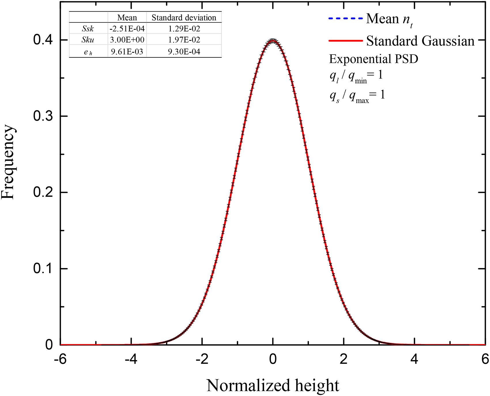
Mean histogram of simulated surfaces and corresponding standard deviation with exponential power spectral density (PSD), q_l /q_min = 1, q_s/q_max = 1.

Simulation of non-Gaussian fractal surfaces

The method of Wang et al.²⁴ was tested to simulate a fractal surface indexed as NG-1 with Ssk = −1 and Sku = 7. Considering the brevity of this paper, we do not include the validation of the method implementation here. Relevant details will be provided according to the requirements of readers. The PSD of the simulated surface was plotted in Figure 16 together with the target PSD. The results show that huge discrepancies exist between the simulated and target PSDs. This phenomenon is very different from the high accuracy reported by Wang et al.²⁴ It is not difficult to infer that the reason behind such different behavior is about altering the exponential PSD to power-law PSD. The procedures used to find the underlying PSD (see section Simulation of non-Gaussian rough surfaces and Wang et al.²⁴) do not work well with the power-law PSD, and the quality of the underlying PSD corresponding to the power-law PSD is poor. Therefore, the Wang et al.²⁴ method is not the proper choice to generate non-Gaussian fractal surfaces.

Figure 16.

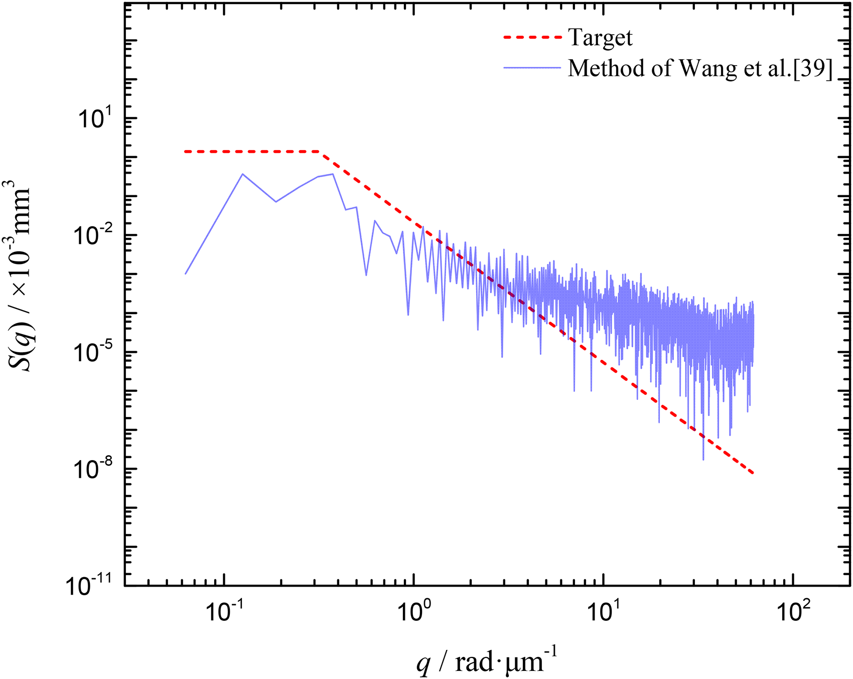
Target power spectral density (PSD) and PSD of one NG-1 fractal surface simulated by the method of Wang et al.²⁴

Based on the attempt to simulate the non-Gaussian fractal rough surfaces above, it can be inferred that the power-law PSD limits the ability of SRM in generating non-Gaussian surfaces. Therefore, a compromise between reproducing the power-law PSD and non-Gaussian height distribution should be made to simulate non-Gaussian fractal surfaces. In that case, what if directly translating simulated Gaussian surfaces to non-Gaussian surfaces by the Johnson translator system?

In the current work, this idea was tested. Firstly, Gaussian fractal rough surfaces were simulated by the SRM. Then, the Gaussian surfaces were translated to non-Gaussian surfaces with the parameters listed in Table 3 by the Johnson translator system. These parameters are chosen to cover the range of Ssk and Sku values of surfaces machined by the most common machining processes.⁴⁶ As the generated Gaussian surfaces are not ideal, some translated surfaces could have significant errors in reproducing Ssk and Sku values, and these surfaces should be discarded and regenerated. It is worth mentioning that Francisco and Brunetiere⁴² provided a hybrid method to improve the accuracy of translated non-Gaussian series. Therefore, if one needs high accuracy non-Gaussian surfaces, the hybrid method is worth trying.

Table 3.

Ssk and Sku values of the simulated non-Gaussian surfaces.

Surface index	Ssk			Sku
Surface index	Target	Simulated	Error/%	Target	Simulated	Error/%
NG-1	−1	−1.037	3.72	7	6.759	3.45
NG-2	−1	−1.033	3.34	14	14.60	4.31
NG-3	−1	−1.085	8.54	25	26.90	7.61
NG-4	1	1.006	0.65	7	6.837	2.32
NG-5	1	1.040	4.01	14	14.12	0.89
NG-6	1.6	1.562	2.40	7	6.902	1.40
NG-7	−1.6	−1.555	2.80	7	6.870	1.85
NG-8	−3	−2.956	1.44	14	13.43	4.06
NG-9	−3	−3.066	2.18	25	24.05	3.80
NG-10	3	3.062	2.08	25	25.92	3.66
NG-11	−4	−4.104	2.59	50	46.86	6.28
NG-12	4	3.915	2.13	50	45.86	8.29

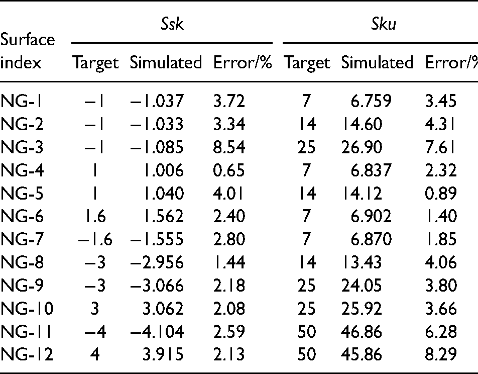
Figure 17 shows the PSDs of surfaces generated by the different parameters in Table 3. It clearly shows that all the PSD curves follow the target power-law PSD approximately. Moreover, although the translation process causes variations in the PSD values, it still gives better agreement with the target power-law PSD than the method of Wang et al.²⁴ (Figure 16). The next task is evaluating the reproduction of the target Ssk and Sku values. The corresponding values of each simulated surface and the relative errors are listed in Table 3 as well. It can be seen that most of the simulated surfaces have relative errors of <5%, and the highest relative error is still <10%, which means a sound reproduction of the target Ssk and Sku values.

Figure 17.

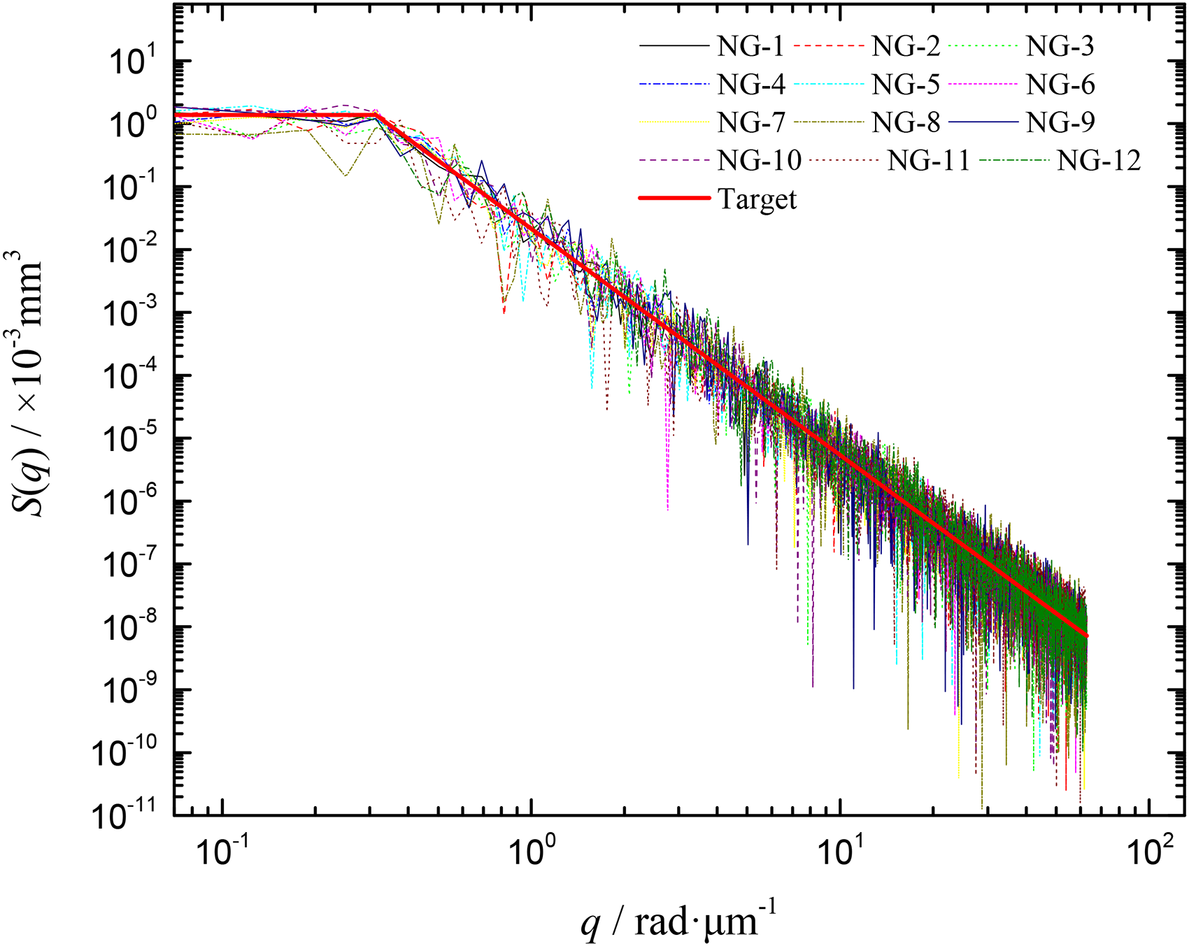
Power spectral density (PSD) values of the simulated non-Gaussian fractal surfaces.

Therefore, by directly translating simulated Gaussian surfaces to non-Gaussian surfaces through the Johnson translator system, a compromise between the accuracy of the PSD and the non-Gaussian height distribution is achieved. This method provides a straightforward way to simulate non-Gaussian fractal surfaces, as no iterative steps are included. One should keep in mind that this method is approximate and can be used when the uncertainties in the PSD do not affect the specific applications much. If high accuracy of the PSD and height distribution is required, some more complex methods should be considered, such as the work of Pérez-Ràfols and Almqvist³⁶ and Francisco and Brunetiere.⁴²

Conclusions

This paper studied the application of the spectral representation method (SRM) in generating Gaussian and non-Gaussian fractal rough surfaces and compared it with the traditional FFT filtering method. The influences of PSD cutoff frequencies were also investigated. The main conclusions are as follows:

The FFT filtering method has two sources of uncertainties theoretically, PSD as the amplitude term and the phase term, which are probably irrelevant according to the preliminary analysis of roughness parameters in this paper.

Compared with the FFT filtering method, the SRM does not introduce uncertainties in the PSD, which gives the SRM advantages in predicting statistical quantities in tribology analysis. One single rough surface generated by the SRM can instead take average results obtained using dozens of surfaces generated by the FFT filtering method, reducing the cost of computation resources significantly. For some applications where the extreme conditions, not averaged results, are important, the FFT filtering method might still be needed to include uncertainties in the PSD.

The ratio of high cutoff frequency, q_s, to the upper bound of the frequency range, q_max, does not significantly affect the normality of simulated Gaussian fractal surfaces.

The ratio of low cutoff frequency, q_l, to the lower bound of the frequency range, q_min, significantly influences the normality of simulated Gaussian fractal surfaces. Increasing the q_l/q_min value can improve the normality of the simulated Gaussian fractal surfaces. Such improvement for the PSD without roll-off is more significant than that for the roll-off PSD. For the PSD without roll-off, the q_l/q_min value shall be at least >1.

Compared with using the power-law PSD, the q_l/q_min has nearly zero effect on the normality of simulated Gaussian surfaces using an exponential PSD, which indicates such influence might be a particular case along with the power-law PSD.

Directly translating Gaussian fractal surfaces simulated by the SRM to non-Gaussian surfaces through the Johnson translator system compromises the accuracy of the PSD to reproduce non-Gaussian properties. It could be used as an approximate but fast method to generate non-Gaussian fractal surfaces when the uncertainties in the PSD do not significantly affect the specific applications.

Footnotes

Acknowledgements

This work was undertaken on ARC3, part of the High-Performance Computing facilities at the University of Leeds, UK.

Declaration of Conflicting Interests

The author(s) declared no potential conflicts of interest with respect to the research, authorship, and/or publication of this article.

Funding

The author(s) disclosed receipt of the following financial support for the research, authorship, and/or publication of this article: This work was supported by the Engineering and Physical Sciences Research Council (grant number EP/001766/1”) as a part of ‘Friction: The Tribology Enigma’ Programme Grant (), and TRibology as an ENabling Technology (TRENT) EP/S030476/1). Supplemental material for this article is available online.

ORCID iDs

Yuechang Wang

Ardian Morina

Appendix

References

Persson

BNJ

. On the fractal dimension of rough surfaces. Tribol Lett 2014; 54: 99–106.

Sayles

Thomas

. Surface topography as a nonstationary random process. Nature 1978; 271: 431–434.

Majumdar

Bhushan

. Role of fractal geometry in roughness characterization and contact mechanics of surfaces. J Tribol 1990; 112: 205–216.

Majumdar

Tien

. Fractal characterization and simulation of rough surfaces. Wear 1990; 136: 313–327.

Ganti

Bhushan

. Generalized fractal analysis and its applications to engineering surfaces. Wear 1995; 180: 17–34.

Peklenik

. Paper 24: new developments in surface characterization and measurements by means of random process analysis. Proc Inst Mech Eng, Conf Proc 1967; 182: 108–126.

Nayak

. Random process model of rough surfaces. J Lubr Technol 1971; 93: 398–39&.

Persson

BNJ

Albohr

Tartaglino

, et al. On the nature of surface roughness with application to contact mechanics, sealing, rubber friction and adhesion. J Phys: Condens Matter 2004; 17: R1–R62.

Müser

Dapp

Bugnicourt

, et al. Meeting the Contact-Mechanics Challenge. Tribol Lett 2017; 65, 118 (2017).

10.

Majumdar

Bhushan

. Fractal model of elastic-plastic contact between rough surfaces. J Tribol 1991; 113: 1–11.

11.

Dapp

Lucke

Persson

, et al. Self-affine elastic contacts: percolation and leakage. Phys Rev Lett 2012; 108: 244301.

12.

Yastrebov

Anciaux

Molinari

J-F

. From infinitesimal to full contact between rough surfaces: evolution of the contact area. Int J Solids Struct 2015; 52: 83–102.

13.

Papangelo

Hoffmann

Ciavarella

. Load-separation curves for the contact of self-affine rough surfaces. Sci Rep 2017; 7: 6900.

14.

Yang

. Surface roughness effects on point contact elastohydrodynamic lubrication in linear rolling guide with fractal surface topographies. Ind Lubr Tribol 2018; 70: 589–598.

15.

Zhang

Jackson

. A mixed lubrication analysis of a thrust bearing with fractal rough surfaces. Proc Inst Mech Eng, Part J: J Eng Tribol 2019; 234: 608–621.

16.

Pawlus

Reizer

Wieczorowski

. A review of methods of random surface topography modeling. Tribol Int 2020; 152: 106530.

17.

Patir

. Numerical procedure for random generation of rough surfaces. Wear 1978; 47: 263–277.

18.

Tonder

. Simulation of 3-d random rough-surface by 2-d digital-filter and Fourier-analysis. Int J Mach Tools Manuf 1992; 32: 83–90.

19.

Bakolas

. Numerical generation of arbitrarily oriented non-Gaussian three-dimensional rough surfaces. Wear 2003; 254: 546–554.

20.

Minet

Brunetiere

Tournerie

, et al. Analysis and modeling of the topography of mechanical seal faces. Tribol Trans 2010; 53: 799–815.

21.

Newland

. An introduction to random vibration and spectral analysis. 2nd ed. London: Longman, 1984.

22.

. Simulation of rough surfaces with FFT. Tribol Int 2000; 33: 47–58.

23.

J-J

. Simulation of non-Gaussian surfaces with FFT. Tribol Int 2004; 37: 339–346.

24.

Wang

Liu

Zhang

Wang

, et al. (October 4, 2017). A Simulation Method for Non-Gaussian Rough Surfaces Using Fast Fourier Transform and Translation Process Theory. ASME. J. Tribol. March March 2018; 140(2): 021403.

25.

Johnson

. Systems of frequency curves generated by methods of translation. Biometrika 1949; 36: 149–176.

26.

Voss

. Random fractal forgeries. Berlin, Heidelberg: Springer Berlin Heidelberg, 1985, pp.805–835.

27.

Voss

. Fractals in nature: from characterization to simulation. In: Peitgen

H-O

Saupe

(eds) The science of fractal images. New York, NY: Springer New York, 1988, pp.21–70.

28.

Saupe

. Algorithms for random fractals. In: Peitgen

H-O

Saupe

(eds) The science of fractal images. New York, NY: Springer New York, 1988, pp.71–136.

29.

. Characterization of fractal surfaces. Wear 2000; 239: 36–47.

30.

Borri

Paggi

. Topology simulation and contact mechanics of bifractal rough surfaces*. Proc Inst Mech Eng Part J-J Eng Tribol 2016; 230: 1345–1358.

31.

Pei

Hyun

Molinari

, et al. Finite element modeling of elasto-plastic contact between rough surfaces. J Mech Phys Solids 2005; 53: 2385–2409.

32.

Bonari

Marulli

Hagmeyer

, et al. A multiscale FEM-BEM formulation for contact mechanics between rough surfaces. Comput Mech 2020; 65: 731–749.

33.

Paggi

Ciavarella

The coefficient of proportionality κ between real contact area and load, with new asperity models. Wear 2010; 268: 1020–9.

34.

Putignano

Afferrante

Carbone

, et al. A new efficient numerical method for contact mechanics of rough surfaces. Int J Solids Struct 2012; 49: 338–343.

35.

Zou

Feng

, et al. A Monte Carlo method for simulating fractal surfaces. Physica A 2007; 386: 176–186.

36.

Pérez-Ràfols

Almqvist

. Generating randomly rough surfaces with given height probability distribution and power spectrum. Tribol Int 2019; 131: 591–604.

37.

Pérez-Ràfols

Almqvist

. On the stiffness of surfaces with non-Gaussian height distribution. Sci Rep 2021; 11: 1863.

38.

Prodanov

Dapp

Müser

. On the contact area and mean gap of rough, elastic contacts: dimensional analysis, numerical corrections, and reference data. Tribol Lett 2014; 53: 433–448.

39.

Shinozuka

Deodatis

. Simulation of stochastic processes by spectral representation. Appl Mech Rev 1991; 44: 191–204.

40.

Watson

Spedding

. The time-series modeling of non-Gaussian engineering processes. Wear 1982; 83: 215–231.

41.

Hill

Holder

. Fitting Johnson curves by moments. Appl Stat 1976; 25: 180–184.

42.

Francisco

Brunetiere

. A hybrid method for fast and efficient rough surface generation. Proc Inst Mech Eng, Part J: J Eng Tribol 2015; 230: 747–768.

43.

Lou

Pagani

Zeng

, et al. Watershed segmentation of topographical features on freeform surfaces and its application to additively manufactured surfaces. Prec Eng 2020; 63: 177–186.

44.

Marklund

Lugt

Almqvist

, et al. A mixed lubrication model incorporating measured surface topography. Part 1: theory of flow factors. Proc Inst Mech Eng, Part J: J Eng Tribol 2010; 224: 335–351.

45.

Venner

Lubrecht

. Numerical analysis of the influence of waviness on the film thickness of a circular EHL contact. J Tribol 1996; 118: 153.

46.

Whitehouse

. Handbook of surface and nanometrology. 2nd ed, Boca Raton, CRC Press, 2010.

Generating fractal rough surfaces with the spectral representation method

Abstract

Keywords

Introduction

FFT filtering method and SRM

Simulation of non-Gaussian rough surfaces

Results and discussion

Surfaces generated by the FFT filtering method and SRM

Contact of rough surfaces

EHL simulation

The influence of low and high cutoff frequencies

Simulation of non-Gaussian fractal surfaces

Conclusions

Footnotes

Acknowledgements

Declaration of Conflicting Interests

Funding

ORCID iDs

Appendix

References