Digital Filtering and Signal Decomposition: A Priori and Adaptive Approaches in Body Area Sensing

Abstract

Elimination of undesired signals from a mixture of captured signals in body area sensing systems is studied in this paper. A series of filtering techniques including a priori and adaptive approaches are explored in detail and applied involving decomposition of signals along a new system’s axis to separate the desired signals from other sources in the original data. Within the context of a case study in body area systems, a motion capture scenario is designed and the introduced signal decomposition techniques are critically evaluated and a new one is proposed. Applying the studied filtering and signal decomposition techniques demonstrates that the functional based approach outperforms the rest in reducing the effect of undesired changes in collected motion data which are due to random changes in sensors positioning. The results showed that the proposed technique reduces variations in the data for average of 94% outperforming the rest of the techniques in the case study although it will add computational complexity. Such technique helps wider adaptation of motion capture systems with less sensitivity to accurate sensor positioning; therefore, more portable body area sensing system.

Introduction

In body area signal processing systems, one of the challenges is elimination of unwanted signals from a mixture of sources that is called filtering. The techniques for removal of undesired signals are commonly using a linear signal decomposition. The method is to present the data in a new space whereas the desired signal is filtered out from other signals in the original signal projected onto different basis vectors or functions. ¹ By retaining the basis describing the desired signal and deleting the rest, signal decomposition is performed.

Body area sensing systems specifically designed for motion capture of walking or gait are measuring human body kinematic variables which are the angles of pelvis, hip, knee, ankle, and foot in the X, Y, and Z axes. Such measured signals which are considered as vectors in time domain for each joint in the direction of the 3 axes are prone to undesired components due to different reasons from varying sensor wearing sessions, inadvertent changes in position of sensors, different walking pattern, and speed, etc. ² Therefore, there is need for removal of undesired components in the captured signals which could be considered and addressed from signal decomposition perspective.

Signal decomposition techniques are categorized into a priori and adaptive ones. It is dependent on the approach that the basis vectors or functions are determined. In a priori approaches the basis are defined independent of the signal, such as finite impulse response (FIR) and infinite impulse response (IIR) filters. The approach is frequency-based utilizing Discrete Fourier Transform (DFT). ³ Such signal decomposition techniques are not used when there is overlap between characteristic frequencies of the undesired signal and the desired signal. To tackle this challenge adaptive frameworks for determining basis vectors or functions have been introduced. ² The basis vectors are calculated from the statistical properties of the data through adaptive approaches including ICA (Independent Component Analysis), PCA (Principal Component Analysis), and SVF (Singular Value Filter) based signal decomposition methods.

The signal decomposition basic principles can be described by initially considering the signal, joint angle in this study, which is represented as a row vector x (dim 1 × N) for each joint angle over the measurement time denoted by N samples. The signals need to be decomposed into a weighted sum of orthonormal basis,

$$\mathbf{x}=\sum _{n=1}^N{c}_n{\mathbf{v}}_n$$

(1)

where $c_n$ are the coefficients for each N orthonormal basis ${\mathbf{v}}_n$ . The inner product between the orthonormal basis vector and the observed signal are represented as coefficients $c_n=$ $\mathbf{x}.{\mathbf{v}}_n^{\prime }$ where ${\mathbf{v}}_n\prime$ is the conjugate transpose of ${\mathbf{v}}_n$ . Any set of mutually orthonormal vectors are the basis represented in (2).

$${\mathbf{v}}_n.{{\mathbf{v}}_m}^{\prime }=\{\begin{array}{c}1,\mathrm{for}n=m\\ 0,\mathrm{for}n\ne m\end{array}$$

(2)

For linear transformation, the mutually orthonormal basis ${\mathbf{v}}_n$ are formulated either through a priori or adaptive approaches from the observed signal. In adaptive methods, the basis vectors or functions are formed adaptively based on a series of polynomials.

A general linear filtering technique for discrete time system is represented through a matrix formulation, y = Ax whereas x =  ${[x\left(0\right),x\left(1\right),\dots ,x\left(N-1\right)]}^{\mathrm{T}}$ is input, y =  ${[\mathrm{y}\left(0\right),\mathrm{y}\left(1\right),\dots ,\mathrm{y}\left(N-1\right)]}^{\mathrm{T}}$ is the output of transform and A which is transform matrix has N × N dimension. Each element of the matrix is represented by $a\left(n,k\right)$ whereas n is the element in the rows and k is the element in columns. Therefore, the transform’s output vector element, $y\left(n\right),$ are represented as (3).

$$y\left(n\right)=\sum _{k=0}^{N-1}a\left(n,k\right)x\left(k\right),n=0,\dots ,N-1$$

(3)

By selecting the first M coefficient and rejecting the rest, $\widehat{y}$ , as represented in (4) the filtered signal, $\widehat{\mathbf{x}}$ , is reconstructed from $\widehat{\mathbf{x}}$  =  ${\mathbf{A}}^{-1}\widehat{y}$ as the process is demonstrated in Figure 1.

$$\widehat{y}\left(n\right)=\sum _{k=0}^{M-1}a\left(n,k\right)x\left(k\right),n=0,\dots ,M-1$$

(4)

Figure 1.

Signal decomposition-based filtering technique process.

The signals could have different characteristics such as being deterministic or random, orthogonal, orthonormal, or independent. A signal is called deterministic if there is no uncertainty about its values at any time which means it can be represented by a mathematical formula as a function of time. A signal is non-deterministic or random if there is uncertainty about its values at some time while being random in nature and are modeled in probabilistic terms. As the aim in this paper is to address random components in the signal, there is need to consider the statistical properties of signals and processes. Stationary process is a procuress that the unconditional joint probability distribution does not change over time; otherwise, the process is non-stationary. Signals are represented as vectors whereas vector space is considered as a set of vectors or functions $\left\{{\mathrm{v}}_n\right\}$ spanning a vector space if any element of that space can be represented as a linear combination of elements of that set $\mathrm{x}={\sum }_{n=1}^N{c}_n{\mathrm{v}}_n$ therefore, $\left\{{\mathrm{v}}_n\right\}$ is a basis set if the c_n is unique. Vectors are orthogonal if the inner product of vectors is zero: $n\ne m,<{\mathrm{v}}_n,{\mathrm{v}}_m>=0$ whereas they are orthonormal if the vectors are orthogonal with unit length: $n=m,<{\mathrm{v}}_n,{\mathrm{v}}_m>=1$ ; a space which has orthonormal basis is a type of Hilbert space where $\mathrm{x}={\sum }_{n=1}^N<\mathrm{x},{\mathrm{v}}_n>{\mathrm{v}}_n$ . In terms of independence, given a set of vectors $\left\{{\mathrm{v}}_i\right\}i=1,2,\dots ,k$ , if there would be a set of $\left\{{\mathrm{c}}_i\right\}i=1,2,\dots ,k$ (excluding $c_1=c_2=\dots =0$ ) such that $c_1{\mathrm{v}}_1+c_2{\mathrm{v}}_2+\dots +c_k{\mathrm{v}}_k=0$ , then the set of vectors is called linearly dependent. If there is none, they are considered independent in a linear manner.

Having introduced the signal decomposition process, the principles of filtering and signal decomposition techniques including a priori and adaptive approaches along with a functional one are explored considering critical evaluation of them in Section 2. The approach is validated for a case study in a body area sensing scenario for motion signals which are angles of joints to investigate the applicability of the techniques within that context in Section 3. In Section 4, results are presented, compared, and analyzed which validates the applicability of the approach for the case study. The paper will be concluded in Section 5 summarizing the findings and the validity of used techniques.

Background of Filtering and Signal Decomposition Techniques

To reduce undesired components in the signals captured from body area sensing systems, a series of signal decomposition techniques are explored which are critically reviewed in this Section. The signals are specifically angles of joints for the purpose of gait analysis whereas applying the techniques is for the purpose of finding characteristic features that represent the main patterns of motion. By eliminating the undesired components there would be reduced variability in signals of body area sensing systems. When considering the applicability of on-body sensing systems for motion capture, there are challenges related to wearer’s comfort. The systems are sensitive to sensors positioning which need uncomfortable tight-fitting attachments and experts for placement/set-up.^4,5 Using such signal decomposition techniques helps wider adaptation of motion capture systems with less sensitivity to accurate sensor positioning; therefore, more portable body area sensing system. Signal decomposition techniques are categorized into a priori and adaptive ones depending on the approach that the basis vectors or functions are determined. In a priori approaches the basis are defined independent of the signal, whereas for the adaptive ones the basis vectors or functions are derived from statistical properties of the data through adaptive approaches which are critically reviewed in this Section.

A priori signal decomposition

The most common a priori filtering approach, where the basis are independent of the data, is Discrete Fourier transform-based filter whereas the basis for different frequencies are a set of complex exponentials. Such filters have been commonly used in signal decomposition literature. ⁶ The frequency response of a filter is described by parameters such as stop band, pass band and cut-off frequencies. In the stopband, the deviation from zero needs to be small while all the frequencies need to be passed unchanged in the passband whereas the ripples need be minimized. The passband cut-off frequency and the stopband cut-off frequency need to be as close as possible in order to have an ideal filter response. Two key methods of signal separation in the a priori category as discussed in following section are Finite impulse response (FIR) and infinite impulse response (IIR) filters.

FIR filters have finite duration impulse response and also are called non-recursive filters or convolutional filters. From the time domain viewpoint, these filters are sometimes called moving average filter whereas the impulse response is finite. A ${(K-1)}^{th}$ order FIR filter output are represented as (5) with input vector size N, and filter order K−1, whereas the output samples number is N+K−1. The frequency response for such filters is $H_0\left(\omega \right)=|H\left(\omega \right){|}^2$ , the Fourier transform of the impulse response of h(n) is represented by $H\left(\omega \right)$ . FIR filters can be categorized as linear phase and minimum phase filters.

$$y\left(n\right)=\sum _{k=0}^{k-1}h\left(k\right)x\left(n-k\right)=\sum _{k=n-K+1}^{n}h\left(n-k\right)x\left(k\right).$$

(5)

The linear phase FIR filter frequency response is written as (6) where $G\left(\omega \right)$ is a real function and $k_1$ and $k_2$ are constants.

$$H\left(\omega \right)=G\left(\omega \right)e^{j(k_1+k_2\omega )}$$

(6)

If a signal x(n) only consists frequencies in the passband, the filtered signal spectrum is $Y\left(\omega \right)\approx X\left(\omega \right)e^{j(k_1+k_2\omega )}$ . It would be equivalent of a constant phase shift in frequency domain, and a time delay of the input signal in the time domain whereas the signal is not distorted. If the impulse response of the filter is symmetrical, a FIR filter with real coefficients has linear phase. The symmetrical constraint on the impulse response is considered for linear phase filters whereas the required order to obtain a specified amplitude response is reduced with no phase constraints. If in filter design process, the amplitude response is the major concern, filters with different phase responses and optimum amplitude response can be designed. Among such filters the one with all its zeros inside unit circle is the minimum phase filter which has the smallest time delay. In addition, the partial energy $E\left(n\right)={\sum }_{k=0}^n|h(k){|}^2$ of the impulse response is maximized leading to the most asymmetric impulse response.

A Kth-order Infinite Impulse Response (IIR) filter is presented by equation (7) where each output sample depends on present and past input samples in addition to the past output samples.

$$y\left(n\right)=-\sum _{k=1}^K{a}_{k}y\left(n-k\right)+\sum _{k=0}^K{b}_{k}x(n-k)$$

(7)

The filter’s impulse response will not fade due to the recursive part, and it is the cause that they are named IIR filters. Considering the steady-state magnitude response characteristics, many techniques are used for design such as Butterworth, Chebyshev type I and II, and Elliptic filters. For filter design there is a compromise between transient time and magnitude response. As discussed, a FIR filter can have linear phase meaning that there would be a constant group delay because of the filter unit-pulse response symmetry. Causal IIR filters due to the infinite duration of unit-pulse response cannot be symmetric; therefore, IIR filter cannot have exactly linear phase. To design filter with sharp transitions between frequency bands or large attenuation are required in the stop band, the required filter length N increases. When constant delay for all frequencies is not required, FIR filters are used. The minimum phase FIR filters are good alternative when the group delay is not important. With the same number of coefficients, a sharper transition between band edges is present for IIR filter than a FIR filter. In terms of realization, IIR filter is much more difficult than the direct, non-recursive FIR filter due to the recursive structure. Considering similar magnitude characteristics, an IIR filter has fewer coefficients than a FIR filter so less memory is required to store the coefficients which is an advantage over FIR. ⁶

Adaptive signal decomposition

The reviewed filtering techniques in previous part fail to achieve a signal separation when there is overlap in the frequencies of the undesired signal and the desired signal. Moreover, the signals may change through space and time; therefore, adaptive approaches for finding out the basis functions are proposed in the literature. Common adaptive signal decomposition techniques for defining basis functions are Independent Component Analysis, ICA, Principal Component Analysis, PCA, and Singular Value Filter, SVF, which are used in blind source separation (BSS) as well. BSS is an approach for retrieving unseen signals or sources from mixtures of the signals. For separating the sources, no prior information about the signals or their combination is available. Instead, the technique considers that different physical processes have signals with predictable relationships; therefore, specific statistical relationships between the sources. ⁷ Such techniques are widely used due to the need for no prior information about the signals. The ability of these filtering techniques in signal decomposition is dependent on source signals statistics. One of the techniques for this purpose is known as PCA whereas assumes orthogonality of the source signals ⁶ while the other one which is known as ICA assumes independence and non-Gaussian-distribution of the source signals. ⁸ The filtering is achieved by selecting the corresponding source signals’ orthogonal or independent basis, adaptively. To remove the signal of interest, the input signal is “projected onto the complement of the predicted signal subspace while to keep the signal of interest and separate it from the other signals, the input signal is projected onto the basis selected to span the desired signal subspace.” ⁹

Independent component analysis

In this section, it is explained how the independent component analysis, ICA, based filtering techniques decompose undesired sources of variation from the signal of interest through transforming them linearly into the ICA component axes and then maximizing the entropy of the data. In addition, the principal component analysis, PCA, based filters are explored whereas the basis are orthogonal directions of greatest variance in the data calculated adaptively from the covariance properties of the data while ICA components could be non-orthogonal. It is discussed that how the singular value filter, SVF is different from the other adaptive techniques by considering a weighting function that calculates filter coefficients from the data in the singular value domain, adaptively.

Independent component analysis is a linear transformation with statistical independent components that captures the fundamental structure of the data in the observed signal. Therefore, finding a linear demonstration of non-Gaussian data. It is based on the assumption that the sources are uncorrelated and mutually independent. If the original source signals are statistically independent and non-Gaussian ICA can reach to an excellent signal separation in comparison to PCA. ⁶ If the source signals are not independent, the technique may not contribute substantial superiority over PCA. ¹⁰ To estimate the mixing coefficients, $a_{ij}$ , based on the information of their independence, ICA can be used leading to separation of the original source signals $s_1(t)$ , . . ., $s_n(t)$ from their mixtures $x_1(t)$ , . . ., $x_n(t)$ where parameters $a_{ij}$ are mixing coefficients as equation (8).

$$x_j=a_{j1}{s}_1+a_{j2}{s}_2+\dots +a_{jn}{s}_n\mathrm{for}\mathrm{all}j$$

(8)

The assumption is that each mixture $x_j$ , and each independent component $s_k$ , are random variable. The model is presented by x, a random vector with elements are the mixtures $x_1(t)$ , . . ., $x_n(t)$ , and s which is a random vector with elements $s_1(t)$ , . . ., $s_n(t)$ and by the matrix A with elements $a_{ij}$ . The mixing is mathematically modeled as x = As using a vector-matrix representation whereas $a_i$ is the column of matrix A which is modeled as (9).

$$\mathbf{x}=\sum _{i=1}^n{\mathbf{a}}_i{\mathrm{s}}_i$$

(9)

For estimating the mixing matrix, A, it is assumed that the components $s_i$ are independent from statistical perspective and the independent components’ distributions are non-Gaussian. By finding out the matrix A, its inverse, W, can be calculated; therefore, the independent components are obtained from s = Wx. By using the technique sources of variation can be separated, so in filtering application the unwanted source of variation can be removed from the signal.

The meaning of independence can be summarized as following. “Variables” $y_1$ and $y_2$ are independent if information on the value of $y_1$ does not give any information on the value of $y_2$ , and vice versa whereas for ICA this is the case with the variables $s_1$ and $s_2$ .” ⁸ Random variables $y_1$ and $y_2$ are independent if and only if the joint probability density function is factorized $p\left(y_1,y_2\right)=p\left(y_1\right)p\left(y_2\right).$ This definition is applied to any number n of random variables; whereas the joint density will be a product of n terms. For independent random variables, the expectancy of $h_1$ and $h_2$ functions will be $E\{h_1(y_1)h_2(y_2)\}$  =  $E\{h_1(y_1)\}E\{h_2(y_2)\}$ . A weaker form of independence is uncorrelatedness whereas 2 random variables $y_1$ and $y_2$ are uncorrelated, if $E\{y_1{y}_2\}$ - $E\{y_1\}E\{y_2\}=0$ . If the variables are independent, they are uncorrelated while uncorrelatedness does not imply independence. ⁸

“Because independence denotes uncorrelatedness, many ICA methods always give uncorrelated estimates of the independent components that reduces the number of free parameters and shortens the problem. The important constraint in ICA is that the independent components must be non-Gaussian for ICA to be possible. In the Gaussian case the density is completely symmetric which means it does not contain any information on the directions of the columns of the mixing matrix A that is the reason for not being able to estimate A. Without non-Gaussianity the estimation of the mixing matrix is not possible.” ⁸

Based on Central Limit Theorem under certain conditions summation of a number of independent random variables would have a Gaussian distribution under certain conditions. In ICA, there is the assumption that there is a mixture of independent components, and the components have identical distributions; therefore, the estimation of one of the independent components involves a linear combination of the $x_i$ which is represented by $y={\mathbf{w}}^{\mathrm{T}}\mathbf{x}$  = ∑ _i $w_i{x}_i$ whereas vector $\mathbf{w}$ is the one to be find out. The linear combination would be equivalent of one of the independent components, if $\mathbf{w}$ would be one of the rows of the independent components. If w were one of the rows of the inverse of A, this linear combination would actually be equivalent of one of the independent components. ⁹

A variable change is considered to determine the estimator giving an approximation for the transform which defines $\mathbf{z}={\mathbf{A}}^T\mathbf{w}$ . Therefore, $y={\mathbf{w}}^{\mathrm{T}}\mathbf{x}={\mathbf{w}}^{\mathrm{T}}\mathbf{A}s={\mathbf{z}}^{\mathrm{T}}\mathbf{s}$ whereas the variable $y$ is linear combination of $s_i$ , with $z_i$ as weights. Because $y$ would be summation of a number of independent random variables its probability distribution would have a more Gaussian distribution than any of the original variables, than any of the $s_i$ and will be least Gaussian when equals to one of the $s_i$ . ¹⁰

Based on information theory, ICA mixing matrix would be estimated through minimization of mutual information. The mutual information I between m (scalar) random variables, $y_i$ , i = 1, . . ., m is defined as (10) where as $H$ is the entropy, the degree of information that an observable variable provides. The entropy is larger when in the data there is more element of randomness, unpredictable and unstructured features.

$$I\left(y_1,y_2,\dots ,y_m\right)={\sum }_{i=1}^{m}H(y_i)-H(y).$$

(10)

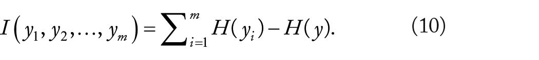
Entropy H is defined for a discrete random variable Y as (11), where the $a_i$ are the possible values of Y.

$$H(Y)=-{\sum }_{i}P\left(Y=a_i\right)\log P(Y=a_i)$$

(11)

A measure of the dependence between random variables is mutual information that is correspondent to the divergence between the joint density f(y) and the product of its marginal densities. If and only if the variables are statistically independent, the entropy is nonnegative, and zero. Therefore, mutual information considers the whole dependence structure of the variables, and not only the covariance which is considered in PCA and related methods. Non-Gaussianity measure which is called negentropy is obtained by defining differential entropy. Negentropy J is defined as $J\left(y\right)=H\left(y_{\mathrm{gauss}}\right)-H(y)$ where $y_{\mathrm{gauss}}$ is a Gaussian random variable of the same covariance matrix as y. In this method, the ICA of a random vector x is defined as an invertible transformation, where the matrix W is determined such that the mutual information of the transformed components $s_i$ is minimized. ¹¹

In multivariate data analysis, finding a smaller number of less redundant variable is the aim, therefore, giving a representation of the original set as possible which is called source separation. However, in PCA and the related Karhunen-Loeve transform the redundancy is measured by correlation between data, in comparison to the ICA with a stronger independence feature with less emphasize on the number of variables. However, in PCA there would, less complexity due to the use of correlation as second order statistics.

Principle component analysis

Decomposing data into its orthogonal basis, the Karhunen–Loeve (KL) transform is used specifying the autocorrelation matrix’s eigenvalues and the relevant orthonormal eigenvectors. ¹² PCA could be useful for filtering such as the one in Negishi, ¹³ but its capability for adaptive regression filtering is restricted. The orthogonal bases of PCA indicates that they are uncorrelated but it does not necessarily mean the statistical independence. “Orthogonal basis are independent only if they are Gaussian or otherwise distributed random variables for which the second and higher order moments are zero.” ⁶ Orthogonal basis are not necessarily mutually statistically independent which means there could be multiple independent sources potentially to be projected onto the same orthogonal basis leading to a source separation which is incomplete.

For PCA transform, there is no assumption on the vector’s probability density whereas the first and second order statistics is estimated. ⁶ Assuming the random vector x with n elements with samples $\mathbf{x}\left(1\right),\dots ,\mathbf{x}\left(T\right)$ , initially the vector x is centered by subtracting its means. The redundancy induced by correlations is removed when x is linearly transformed to another vector y with m elements, where m < n. The PCA transformation is achieved by either variance maximization or by minimum mean-square error compression, MSE.

Variance maximization approach is about a linear combination is considered where as $y_1$ = ${\sum }_{k=1}^n{\omega }_{k1}{x}_k$ = ${\omega }_1^T$ x of the elements $x_1$ , . . ., $x_n$ of the vector x, the ${\omega }_{11}$ , . . ., ${\omega }_{n1}$ are scalar coefficients of an n-dimensional vector ${\omega }_1$ and ${\omega }_1^T$ represents the transpose of ${\omega }_1$ . The factor $y_1$ is called the first PC of x, if the variance of $y_1$ is maximally large. Since the variance depends on both the norm and orientation of the weight vector ${\omega }_1$ and increases without limits as the norm increases, it causes the constraint that the norm of ${\omega }_1$ is constant and equal to 1, practically. Thus, looking for a weight vector ${\omega }_1$ that maximizes the PCA criterion

$$\begin{array}{c}{J}_1^{PCA}\left({\omega }_1\right)=\mathrm{E}\left\{y_1^2\right\}=\mathrm{E}\{({\omega }_1^T\mathbf{x}{)}^2\}={\omega }_1^T\mathrm{E}\{\mathbf{x}{\mathbf{x}}^T\}{\omega }_1\\ ={\omega }_1^T{\mathbf{C}}_{\mathrm{x}}{\omega }_1\mathrm{that}\left|\right|{\omega }_1\left|\right|=1.\end{array}$$

(12)

The ${\omega }_1$ norm is defined as || ${\omega }_1$ ||= ${({\omega }_1^T{\omega }_1)}^2$ which is Euclidean norm. The matrix ${\mathbf{C}}_{\mathrm{x}}$ is the n× n covariance matrix of x given for the zero mean vector x by the correlation matrix ${\mathbf{C}}_{\mathrm{x}}$ = E{x ${\mathbf{x}}^T$ }. The solution to the PCA problem is given in terms of the unit length eigenvectors $e_1$ , . . ., $e_n$ of the matrix ${\mathbf{C}}_{\mathrm{x}}$ based on the linear algebra. The ordering of the eigenvectors is such that the corresponding eigenvalues ${\lambda }_1$ , . . ., ${\lambda }_{1n}$ satisfy ${\lambda }_{11}$ ⩾ . . . ⩾ ${\lambda }_{1n}$ . The solution for the maximization problem is ${\omega }_k=e_k$ . Another approach to compute the basis is eigenvalue decomposition on the autocorrelation matrix,

$$\mathbf{R}=\mathbf{X}\prime \mathbf{X}=\mathbf{V}\Lambda \mathbf{V}\prime$$

(13)

where the matrix $\Lambda$ is a diagonal matrix with the kth element is the kth eigenvalue. Eigenvalues are positive and real which are usually arranged in descending value order. For each eigenvalue, there is an associated eigenvector, which is contained in the columns of $\mathbf{V}$ corresponding to the PCA basis. The kth eigenvalue is proportional to the amount of variance accounted for by the kth eigenvector ${\lambda }_k={\Vert X{\mathbf{v}}_k^{,}\Vert }^2$ . Instead of eigenvalue decomposition, there is another approach to perform a singular value decomposition (SVD) without computing the autocorrelation matrix. The SVD of $\mathbf{X}$  = U ∑ $V\prime$ is where columns of U are the singular vectors corresponding to the eigenvectors of $XX\prime$ and ∑ is a diagonal matrix of singular values ${\sigma }_k$ with singular values arranged in descending value order. ⁶

MSE approach defines compression of x as PCA as weighted sums of the element x with maximal variance whereas the weights need to be normalized. In this approach, m orthonormal basis are selected that are spanning an m-dimensional subspace to minimize the MSE between x and its projection on the subspace that is represented by (14).

$$J_{MSE}^{PCA}=E\left\{\right|\left|\left(x-\sum _{i=1}^m({\omega }_i^T\mathbf{x}){\omega }_i\right)\right|{|}^2\}$$

(14)

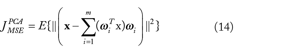
Due to orthogonally of the vectors ${\omega }_i$ , this criterion can be further written as

$$\begin{array}{c}{J}_{MSE}^{PCA}=E\left\{{\left|\left|x\right|\right|}^2\right\}-E\left\{{\left|\left|{\sum }_{j=1}^m({\omega }_i^{T}x){\omega }_i\right|\right|}^2\right\}\\ =\mathrm{trace}(C_{\mathrm{x}})-{\sum }_{j=1}^m{\omega }_j^T{C}_{\mathrm{x}}{\omega }_j.\end{array}$$

(15)

Assuming orthonormality condition on the ${\omega }_i$ for PC orthonormal basis, the subspace spans by the m first eigenvectors $e_1$ , . . ., $e_m$ of $C_{\mathrm{x}}$ derived from (16). The variance of the PCs is calculated by the eigenvalues of $C_{\mathrm{x}}.$

$$\mathrm{E}\left\{{\mathrm{y}}_{\mathrm{m}}^2\right\}=\mathrm{E}\left\{e_{\mathrm{m}}^{\mathrm{T}}x{x}^{\mathrm{T}}{e}_{\mathrm{m}}\right\}=e_{\mathrm{m}}^{\mathrm{T}}{C}_{\mathrm{x}}{e}_{\mathrm{m}}={\mathrm{d}}_{\mathrm{m}}.$$

(16)

Singular Value Decomposition is another technique whereas weights to the basis of PCA decomposition to achieve filtering output is considered. ¹⁴ In this approach, the filter coefficients are function of the data singular value spectrum. In reviewed PCA-based filtering techniques in previous sections, weightings are restricted to 0 and 1 which means each basis function is either deleted or kept. However, based on statistical properties of the signal a weighting function is considered. ¹⁵ The filter coefficients will cause consistent and better filtering results because of eliminating undesired signal components with blocking of artifacts caused by strict thresholding. After decomposing the signal along a new set of PCA basis, filtering is addressed by allocating weights to each of the basis as (17).

$$y=\sum _{k=1}^N{\omega }_k{\gamma }_k{v}_k$$

(17)

where y is the output signal of the filter with the same dimensions as x. The filter coefficients, ${\omega }_k,$ are adaptively calculated as a function of the singular value spectrum as stated in equation 18.

$${\omega }_k={\omega }_k\left({\sum }^{}\right)=1-\frac{1}{1+e^{-\alpha ({\sum }^{}-\tau )}}$$

(18)

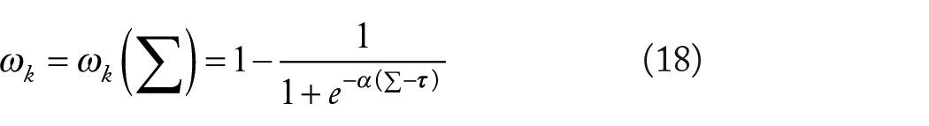
In this equation, $\tau$ and $\alpha$ are weighting function parameters determining the cut-off threshold and weighting function smoothing, respectively. The diagonal matrix of singular values, ${\sigma }_k$ , are represented “by ∑. As $\propto \to 0,$ ${\omega }_k\left({\sum }^{}\right)$ flattens, indicating that all basis are kept at the same level and no filtering is obtained. At the other limit as $\propto \to \infty$ , filtering is reached through strict thresholding where ${\omega }_k\left({\sum }^{}\right)$ are binary meaning that basis functions are deleted if the associated singular values have a ∑ value above threshold $\tau$ and kept if ∑ is below the threshold.” ¹⁴

Functional component analysis

Representing PCs by functions rather than vectors will lead to Functional Principal Component Analysis, fPCA. By observing the entire waveform data, this tool will be able to recognize more detailed pattern differences. ¹⁶ PCs provide indications for identifying potentially important differences in the curves. Smoothness is the core to this approach whereas in time domain the nearby values are linked and not differ largely. fPCA is a useful tool for analyzing data providing a recognition mean for the main source of variability of a set of curves.

Within linear transformations, which are computationally easier among multivariate statistical transforms, the use of functional techniques could provide additional understanding into differences in data by considering the data as functions maintains all the information contained in the raw data. A set of functional building blocks are used ${\varnothing }_k$ , $k=1,2,\dots ,K$ , called basis functions combined linearly to fit a function to raw data y as equation (19) called basis function expansion of function x(t).

$$x\left(t\right)=\sum _{k=1}^K{c}_k{\varnothing }_k$$

(19)

Parameters $c_k$ are the coefficients of the expansion. The maximum number of PCs in the multivariate case is the number of variables, whereas in fPCA the number of eigenfunctions is equal to the minimum of K and N, where K is the number of basis functions, and N is the number of variables. ¹⁶ Coefficients $c_k$ are computed through 2 strategies which are smoothing by regression analysis and smoothing by roughness penalties. Smoothness is achieved by defining the data fitting as the minimization of the sum of squared errors which is represented in (20).

$$y_j=x\left(t_j\right)+{\epsilon }_j=c\prime \varnothing \left(\mathrm{t}\right)+{\epsilon }_j=\varnothing \prime (t_j)c+{\epsilon }_j$$

(20)

The raw data vector, y, comprises the n values to be fitted, vector $\epsilon$ contains the corresponding true residual values, and n by K matrix $\varnothing$ contains the basis function values ${\varnothing }_k(t_j)$ . Then there is $y=\varnothing c+\epsilon$ . The least-square estimate of the coefficient vector c is shown in (21).

$$\widehat{c}={(\varnothing \prime \varnothing )}^{-1}\varnothing \prime y$$

(21)

There is no particular limitation on the number of variables N to fit the functions into. The number of basis functions K must be less than or equal to the number of sampled data points, n. An accurate representation of sampled data is achieved when K = n in selecting the coefficients $c_k$ in reaching $x\left(t_j\right)=y_j$ for each j. A better fit to the data is provided by a larger K however the smaller values the less computation is required. ¹⁶ The next stage is calculation of the variance-covariance function, $v(s,t)$ defined as (22).

$$v\left(s,t\right)=N^{-1}\sum _i^N{y}_i\left(s\right)y_i\left(t\right)$$

(22)

The functional eigenequation is

$${\int }^{}v\left(s,t\right)\xi \left(t\right)dt=\rho \xi \left(s\right),$$

(23)

where $\rho$ is eigenvalue and $\xi \left(\mathrm{s}\right)$ is an eigenfunction of the variance-covariance function. ¹⁶ The eigenfunction s called the principal component weight function, ${\xi }_1(\mathrm{s})$ is calculated by (24).

$$\begin{array}{l}\mathrm{Maximize}\sum _i{f}_{i1}^2\\ \mathrm{Subject}\mathrm{to}{\int }^{}{\xi }_1^2\left(s\right)ds={\Vert {\xi }_1\Vert }^2=1,\end{array}$$

(24)

where the PC score $f_{i1}$ is defined as

$$f_{i1}={\int }^{}{\xi }_1\left(\mathrm{s}\right)x_i\left(\mathrm{s}\right)ds.$$

(25)

A non-increasing sequence of eigenvalues ${\rho }_1\ge {\rho }_2\ge \dots \ge {\rho }_k$ can be built step by step by needing each new eigenfunction computed to be orthogonal to those computed in the previous steps,

$$\begin{array}{l}{\int }^{}{\xi }_j\left(t\right){\xi }_l\left(t\right)dt=0,j=1,\dots ,l-1\\ {\int }^{}{\xi }_l^2\left(t\right)dt=1.\end{array}$$

(26)

Separating signals into deterministic and stochastic components, fPCA can be used that is achievable by deducting either one or other from the signal and can be considered as filtering the noise or the common parts, respectively. The approach is to re-present the original data along a new coordinate system such that the signal of interest can be decomposed from other sources of variation in the original data while projecting the signal along different basis. By retaining the basis describing the signal of interest and deleting the remaining, the filtering is accomplished. ²

The signal processing pipeline consists of several stages. Data needs to be normalized in the first step to ensure the same number of samples. Then transferring the data to the fPCA domain by using the fPCA transform and partitioning the data into 2 elements, ${\overrightarrow{x_i}}^{(global)}$ and ${\overrightarrow{x_i}}^{(filtered)}$ as shown in equation (27).

$$\begin{array}{c}\overrightarrow{x_i}={\overrightarrow{x_i}}^{(global)}+{\overrightarrow{x_i}}^{(filtered)}\\ ={\sum }_{n=1}^{L<NE}{\xi }_n(\mathrm{t})f_i^{(n)}+{\sum }_{n=L+1}^{NE}{\xi }_n(\mathrm{t})f_i^{(n)}\end{array}$$

(27)

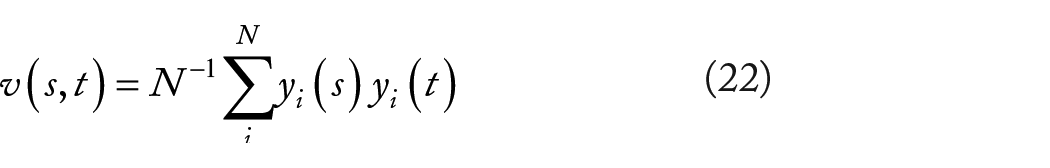
The filter characteristic depends on the data because the sum of the major PCs weight functions is given by ${\overrightarrow{x_i}}^{(global)}\mathrm{and}$ number of eigenfunctions, ${\xi }_n\left(\mathrm{t}\right),$ defining the global pattern affects the filtered pattern as well as the sum of the residual components that is shown by ${\overrightarrow{x_i}}^{(filtered)}$ . In (27), principal component scores are shown by $f_i^{(n)}$ . The number of eigenfunctions is shown by NE and the number of selected ones is shown by L.

After applying fPCA on the data, the main source of variation in the data is filtered by keeping the components containing the most amount of variability through the most relevant PC function or eigenfunctions and removing the rest from the fPCA domain. After this stage, by projecting the data on the retained eigenfunctions the data will be returned to the first domain. The dominant modes of variation in the data can be kept by studying the ratio of the related eigenvalues to the total variance while deducting the mean from each observation. Consistent features are coherent components generating common structures and following deterministic rules, while there is a degree of randomness or stochasticity in the residual components. ¹⁸

Methodology

The signal decomposition and filtering techniques are explored to compensate for the random changes effect in the sensors’ positioning in motion data to find characteristic features that represent the main patterns of motion. Investigating applicability of the signal decomposition techniques, a series of experiments are designed for a motion capture scenario for the purpose of gait analysis whereas the signals are angles of joints including pelvis, hip, knee, ankle, and foot in X, Y, and Z directions. Ten subjects are hired to walk in 10 sessions of sensor wearing with feigned changes in sensors positioning. ² An appropriate number of subjects are required to be recruited to have a valid analysis of motion data. In a similar scenario in the literature for gait analysis, 7 subjects are used based on statistical power analysis ¹⁷ ; therefore, in our experiments it is decided to recruit 10 subjects, 5 females, and 5 males. A power analysis can be used to estimate the minimum sample size required for an experiment, given a desired significance level, effect size, and statistical power which is the probability of a hypothesis test of finding an effect if there is an effect to be found.

Inadvertent changes are emulated in the sensors position for each session while following the standard marker set. There are several standard marker-sets for placing markers on the human body such as Cleveland Clinic, Saflo, Helen Hayes, Codamotion, and so forth. The Cleveland Clinic marker set uses a rigid triad of markers in a plane parallel to the long axis of the bone to capture the motion of the thigh and shank in 3 dimensions. The Saflo marker-set consists of a total body marker-set with 19 retro-reflective markers fixed on specific anatomic landmarks. The Helen Hayes marker set is a relatively simple set of external markers developed for time-efficient video analysis of lower extremity kinematics. All the named marker placement protocols are used for clinical gait analysis. For measuring bilateral gait, the recommended Codamotion marker-set is used which comprises a total of 22 standard markers as shown in Figure 2 for the right side of the body. Markers shown in parentheses () are optional. The marker set determines ankle and knee joint centers and segment coordinate systems by means of a marker on a post or wand protruding from the anterior aspect of the thigh and shank, and by single markers placed over the lateral aspect of the joint flexion/extension axis.

Figure 2.

Position of markers on human body for the experiment setup. ⁶

After installing the sensors on legs and pelvis of the subject according to the Codamotion marker-set, the body angles are measured. A motion capture system measures the angles of joints and provides a stick figure view for the subject under experiment as shown in Figure 3. The system is a general-purpose 3-dimensional (3D) motion tracking system called Codamotion. The measurement unit contains 3 pre-aligned solid-state cameras which track the position of a number of active markers, that is, infrared light emitting diodes (LEDs), in real-time. Sampling rates are selectable from 1 Hz up to 200 Hz, dependent on the numbers of markers in use. Each scanner unit contains 3 special cameras which detect infrared pulses of light emitted by the markers and locate the marker positions with very high resolution. The cameras are rigidly mounted on the scanner units so that the system can be pre-calibrated.

Figure 3.

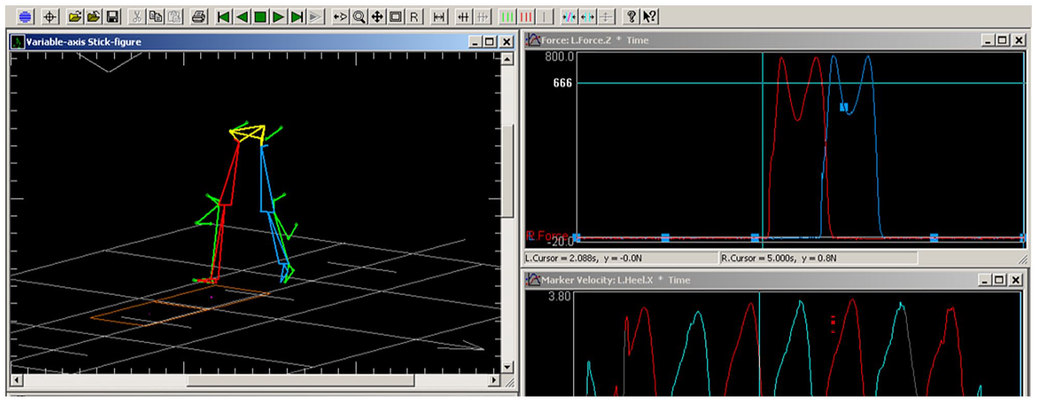
Stick figure and captured signals from force plate, left heel in Z direction to separate each walking step.

The calibrated system measures the positions of markers within a 3D coordinate system that is fixed in relation to the scanner unit. The active range of the capturing system is 1.5 to 5.2 m from the scanners and follows a Gaussian distribution function so that optimal visibility occurs at approximately 3 m from each scanner. The angular resolution of each camera is about 0.002°; this results in a lateral position resolution of about 0.05 mm at 3 m distance (horizontally and vertically), and a distance resolution of about 0.3 mm. The set-up of the motion capture system in the laboratory ensures that all experiments are carried out in this range. The motion capture system will generate angles of joints using the measured sensors/markers positions and the subjects’ body measurements including height and weight.

A random number generator with uniform probability distribution to generate random position displacements is utilized for the purpose of inadvertent changes in the position of sensors. The changes are within the radius of 2 cm in each 10 experiment sessions that the sensors are wore considering the random changes. Despite of the precision in sensor placement regime, there still exists human error in placing sensors whilst following the derived random position obtained from the random number generator. However, we do not consider this source of error further, believing to be relatively small. Each sensor wearing session consists of 6 trials of subjects walking from the initial point to an end point of the walkway while the motion capture system collects the subject’s motion. The Duration of each trial is 5 seconds with 200 Hz sampling rate. The walking speed is asked to be as normal as possible whilst different sensors perturbations are made across different sensors wearing sessions.

The kinematic variables in the experiments on the human subjects are in 3 different Cartesian directions for the angles of pelvis, hip, knee, ankle, and foot. To eliminate the effect of other sources of variation that are not related to sensors positioning differences in each sensor wearing session, the kinematics variables of each sensor wearing session are averaged over the 6 trials. There could be different walking speed, and different ways of walking for each subject and could be the potential reason for such variabilities. Walking is partitioned into cycles whereas each cycle comprises 2 steps whereas a subject is asked to walk for a specific time interval and divide it into cycles. Each walking cycle is considered as the time from initial contact of the heel with the ground to initial contact of the following step. The following right heel contacts are used to separate each step which can be determined from right heel sensor position in Z direction as shown in Figure 3.

There could be different numbers of samples in each walking cycle that is challenging in identifying features during action sequences. For this purpose, each cycle needs to be normalized, so it is denoted by the same sample number. The data is time normalized to convert the time axis from the recorded time units to an axis representing the walking cycle from 0% to 100%. After time normalization, data standardization is performed so that comparing results of different angles with each other in terms of percentage of change before and after applying the filtering techniques. In this case study results of applying fPCA, ICA, PCA, and SVF adaptive filtering techniques and an a priori FFT based filtering mechanism are compared.

Result and Discussion

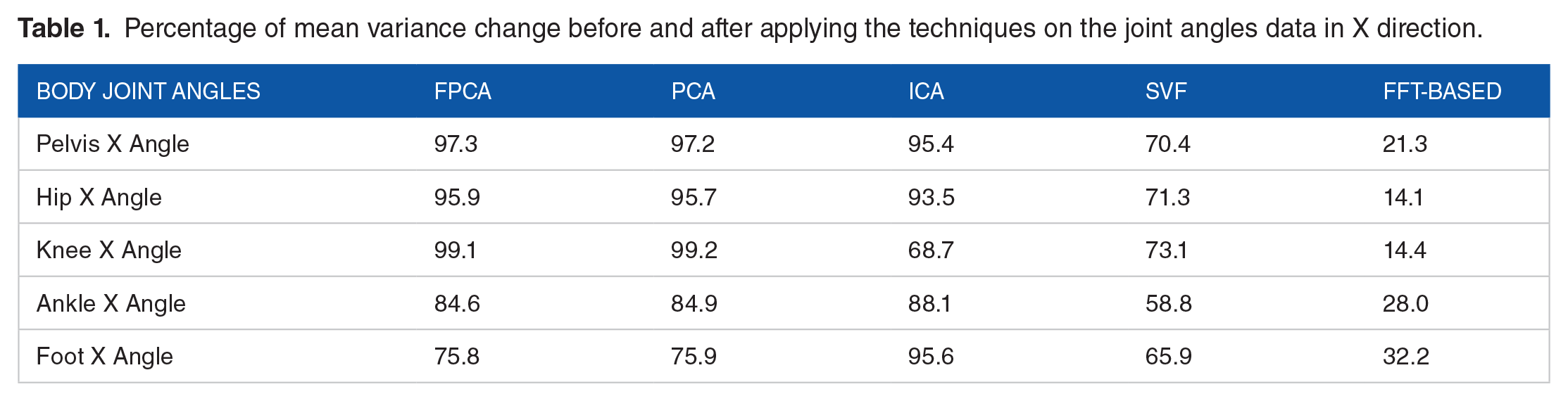
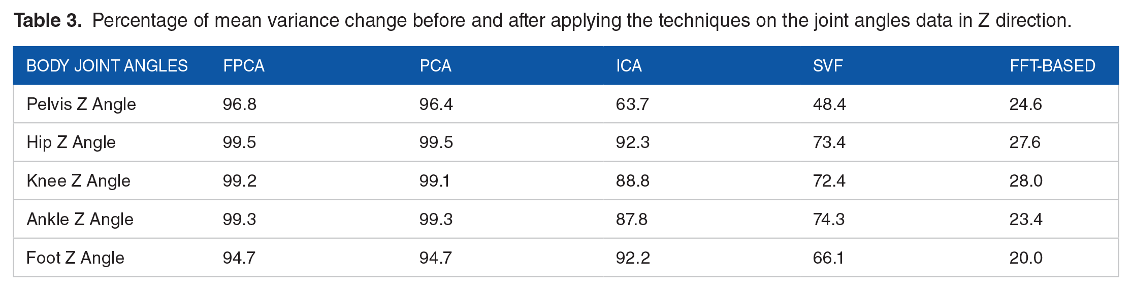
The effect of applying the filtering techniques (fPCA, PCA, ICA, SVF and FFT based) on different angles including pelvis, hip, knee, ankle, and foot as the percentage of mean improvement is listed in Tables 1 to 3 for normalized data in 3 different directions of the Cartesian Coordinate system, respectively. In addition, the right hip angle in the X direction for 10 subjects is shown in Figures 4 and 5 before and after applying the techniques. Motion data is averaged over 6 trials of 10 sessions of marker wearing for each joint angle on 10 human subjects. We can see that for each subject fPCA and PCA schemes are better at separating the main variation pattern in the motion data than other techniques. The Figures confirm consistency in performance of the proposed functional signal separation technique in compensating for positional uncertainties for all participants in the experiment.

Table 1.

Percentage of mean variance change before and after applying the techniques on the joint angles data in X direction.

Body Joint Angles	fPCA	PCA	ICA	SVF	FFT-based
Pelvis X Angle	97.3	97.2	95.4	70.4	21.3
Hip X Angle	95.9	95.7	93.5	71.3	14.1
Knee X Angle	99.1	99.2	68.7	73.1	14.4
Ankle X Angle	84.6	84.9	88.1	58.8	28.0
Foot X Angle	75.8	75.9	95.6	65.9	32.2

Table 2.

Percentage of mean variance change before and after applying the techniques on the joint angles data in Y direction.

Body Joint Angles	fPCA	PCA	ICA	SVF	FFT-based
Pelvis Y Angle	74.7	74.6	90.8	58.4	20.2
Hip Y Angle	99.2	99.2	89.2	68.7	31.8
Knee Y Angle	99.6	99.6	83.0	74.7	14.6
Ankle Y Angle	92.0	91.0	84.9	74.9	18.0
Foot Y Angle	99.7	99.7	84.0	74.8	10.3

Table 3.

Percentage of mean variance change before and after applying the techniques on the joint angles data in Z direction.

Body Joint Angles	fPCA	PCA	ICA	SVF	FFT-based
Pelvis Z Angle	96.8	96.4	63.7	48.4	24.6
Hip Z Angle	99.5	99.5	92.3	73.4	27.6
Knee Z Angle	99.2	99.1	88.8	72.4	28.0
Ankle Z Angle	99.3	99.3	87.8	74.3	23.4
Foot Z Angle	94.7	94.7	92.2	66.1	20.0

Figure 4.

Right hip angle in X direction before and after applying fPCA, PCA, ICA, SVF and FFT for Subject 1 (S1), 2(S2), 3(S3), 4(S4), and 5(S5), respectively.

Figure 5.

Right hip angle in X direction before and after applying fPCA, PCA, ICA, SVF and FFT for Subject 6 (S6), 7(S7), 8(S8), 9(S9), and 10(S10), respectively.

Among a priori FFT based filters, Butterworth IIR filter is selected as a frequency-based filter which is commonly used as a baseline for comparison in literature. A second order low-pass digital filter is used with normalized cut-off frequency of 0.1 Hz to remove high frequency noise. Normalized cut-off frequencies take a variable in range of 0 to 1, where 1 corresponds to the Nyquist frequency. Results show that FFT-based filtering techniques perform poorly on the motion data of our experiments, as expected. As it is shown the mean change percentage in motion data variance before and after applying the technique is 21.94%. Singular value filtering results show mean variance after applying the technique is 68.4 % on average. For ICA based filtering results shows the percentages of change before and after applying the technique is 86.2%. Although the percentage of change is high cases, we see new patterns of variation in the signal which shows that independent component analysis filtering-based techniques are not applicable to this type of data. ¹⁹ Results of applying the PCA-based filtering techniques shows that the technique works properly to reduce random patterns in the data. The percentage of improvement as mean percentage change in both PCA and fPCA is 94%. However, looking specifically into the angles the minimum variance reduction is 88.2% for pelvic angle in Y direction and the maximum improvement is 99.6% for knee angle in Y direction.

The aim in this study is to separate the main pattern of variation in the data from residual components in on-body sensing systems by using signal separation techniques. Results demonstrate as random changes in sensors positioning which are potentially due to undesired movement of wearable sensors, are introduced the motion data variation increases. Before and after applying the filtering techniques, improvement is observed as a percentage of variance changes in the data. Since FFT based filtering projects signals onto frequency components, as shown in results Section it cannot separate the main pattern of variation in the signal from the random variations, which is in the same frequency domain. After applying ICA based techniques, we see some new ripples in the data that are unrelated to the motion patterns. As ICA works on non-Gaussian distributed data, ²⁰ it cannot obtain appropriate results after applying this signal separation technique on the captured data.

The variation in data is due to random changes in sensors positioning. Randomness in the position of sensors is generated using a discrete uniform distribution, which has a symmetric probability distribution that is causing Gaussian distribution of sampled motion data. The SVF-based signal separation performs not better than ICA one which is due to the fact the dominant mode of variance in the data is reflected in the first few principal components. It is evident that the performance of fPCA and PCA is similar in outperforming the rest of the reviewed filtering techniques in stochastic separation of patterns in the data. This can be explained in terms of sampling frequency. As the sampling rate is 200 Hz while the movement pattern bandwidth is around 10 Hz according to the normal walking speed of subjects and movement patterns in data, fitting the function into highly sampled data does not have significant effect. Therefore, in highly sampled data it suggests the use of PCA instead of fPCA as it is easier to perform, and it needs less calculations.

In terms of computational complexity of fPCA algorithms, we can find the coefficients $c_k$ and all smooth values at $x(t_j)$ in $\mathrm{O}(n\log n)$ operations. This efficiency is possible because of the Fast Fourier Transform making it a traditional choice for long time series signal decomposition. As the main difference between PCA and fPCA based techniques is finding the coefficients and smoothing values, the computational complexity of the fPCA based technique is 2 $O(n\log n)$ operations larger than the PCA based technique. We multiplied it by 2 because we first fit the function to data and smooth it, next we perform PCA on the coefficients and then, after applying the filtering technique and transferring the trajectories onto the first domain, we fit the function again to the discrete data. If we consider the data matrix that we apply PCA on as an n by m matrix (n number of samples and m the dimensionality) to compute PCA, we need to compute the covariance matrix and then apply SVD to it. ²¹ The time complexity of computing the covariance matrix is $O(\log \left(n{m}^2\right))$ and then computing SVD is $O(m^3)$ . Therefore, in the procedure of applying the technique for the PCA part, the total time complexity is 2( $O\left(\log \left(n{m}^2\right)\right)+$ $O(m^3)$ ). ²² Multiplication by 2 is for a similar reason that we explained in previous paragraph. Consequently, for applying the fPCA based filtering technique the computational complexity is 2( $O\left(n\log n\right)+O\left(\log \left(n{m}^2\right)\right)+$ $O(m^3)$ ).

Conclusion

Within the context of on-body sensing systems, digital filters and signal decomposition techniques including a priori and adaptive ones were studied. A novel way of using functional principal component analysis was introduced. In this approach, the main variation source in the data is filtered by restoring the most dominant principal components and deleting the remaining from the projected domain. The data will be reverted to the first domain by projecting the data of the retained eigenfunctions and removing eigenfunctions with less variation. However, adding processing complexity to the motion capture procedure is the drawback of the approach. A case study on body area sensing system for motion capture is presented in which the challenge of effect of random changes in sensor placement was explored using the filtering techniques. The results showed that the proposed fPCA based technique reduces variations in the data for average of 94% outperforming the rest of the techniques in the case study although it will add computational complexity. However, by recent advancements in development of cheap and small high power processors this problem can be addressed. The focus in this paper was on human gait; however, future work could be about applying and investigating the introduced signal processing approach for other body movements to validate its applicability for such situations.