Sage Journals: Discover world-class research

Abstract

Rare events such as genetic mutations or cell-cell interactions are important contributors to dynamics in complex biological systems, eg, in drug-resistant infections. Computational approaches can help analyze rare events that are difficult to study experimentally. However, analyzing the frequency and dynamics of rare events in computational models can also be challenging due to high computational resource demands, especially for high-fidelity stochastic computational models. To facilitate analysis of rare events in complex biological systems, we present a multifidelity analysis approach that uses medium-fidelity analysis (Monte Carlo simulations) and/or low-fidelity analysis (Markov chain models) to analyze high-fidelity stochastic model results. Medium-fidelity analysis can produce large numbers of possible rare event trajectories for a single high-fidelity model simulation. This allows prediction of both rare event dynamics and probability distributions at much lower frequencies than high-fidelity models. Low-fidelity analysis can calculate probability distributions for rare events over time for any frequency by updating the probabilities of the rare event state space after each discrete event of the high-fidelity model. To validate the approach, we apply multifidelity analysis to a high-fidelity model of tuberculosis disease. We validate the method against high-fidelity model results and illustrate the application of multifidelity analysis in predicting rare event trajectories, performing sensitivity analyses and extrapolating predictions to very low frequencies in complex systems. We believe that our approach will complement ongoing efforts to enable accurate prediction of rare event dynamics in high-fidelity computational models.

Keywords

Monte Carlo Markov chain stochastic models multifidelity rare events

Introduction

Studying rare events, such as mutation or gene expression, in complex biological systems is challenging because large samples and costly analysis are often required to detect a sufficient number of events. Computational models can help address this challenge by simulating these biological systems. Such computational models can then be applied to more quickly and cost-effectively explore large experimental design spaces. Nonetheless, detailed computational models often suffer from similar barriers as experimental systems; ie, large numbers of simulations are often required to observe these rare events, requiring significant computational time and resources to acquire sufficient data.¹ In this work, we describe a means to circumvent some of these computational challenges, to facilitate efficient experimental design and data analysis. We develop and illustrate a multifidelity analysis approach, incorporating medium-fidelity (MF) analysis (Monte Carlo simulations) and low-fidelity (LF) analysis (Markov chain models) to analyze output from computationally intensive stochastic simulations (high-fidelity [HF] models). We focus on stochastic HF models due to their utility in capturing discrete events, a key feature when studying rare events.

High-fidelity, high-computational-cost models simulate systems with high levels of mechanistic detail. Lower-fidelity models (or surrogate models) of the same system can be used to approximate system dynamics, while eliminating some of the mechanistic details, thereby lowering the computational cost.² Various approaches have been employed to accelerate the simulation of rare events in HF computational models, including weighted ensemble simulations, partitioning, and tau-leaping.^1,3 Multifidelity models or surrogate models can also be used to simulate and approximate complex system dynamics.^4,5 Tunable resolution uses data from fine-grained, mechanistically detailed models to strategically coarse-grain subsections of the fine-grained models as appropriate for various analyses.^6,7 These methods typically consist of HF models and LF models running independently, either for different areas of parameter space or for different regions of interest within a single simulation.^2,4,7,8

Instead, our approach complements these established methods using lower-fidelity models to analyze output from individual simulations of the HF model. Each HF model simulation produces a set of transitions (timing, type, and number of transitions). This set of transitions maps out a finite state space in the rare event coordinate. Our multifidelity analysis then approximates the state probabilities for this entire rare event state space over time based on the set of transitions. In other words, we assume that system transitions in all coordinates except the rare event coordinate are determined by the HF model simulation. This approach expands on the rare event parameter ranges and types of analyses that can feasibly be explored using the HF model alone. For example, in stochastic models, it could be of interest to discern the influence of stochasticity, which we cannot control, from the influence of parameters that we might be able to control through treatment or other interventions. We will first describe our multifidelity approach in light of a simple illustrative example and then show the application of multifidelity analysis to an HF model of drug-resistance emergence in tuberculosis (TB) disease.

Multifidelity Analysis

To illustrate our approach, we consider the example of rare genetic mutations in a population of bacteria that are dividing and dying over time. An HF model of this system could incorporate any number of mechanistic details driving bacterial division and death, eg, available nutrients, influence of surrounding bacterial species, antibacterial chemicals, and host immune responses (Figure 1A).^9–11 Each simulation of such an HF model would produce as output a population trajectory (in this example, the number of bacteria over time). Such a population trajectory is the combined result of 2 series of discrete events: number of bacterial divisions per time unit and number of bacterial deaths per time unit. Because we consider stochastic models, repeated simulations of the same model will result in different population trajectories.

Figure 1.

(A) Hypothetical HF model describing bacterial growth and mutation. Model inputs include mechanistic details driving the population growth (eg, available nutrients). Model outputs include population trajectories (number of bacteria over time) and rare event trajectories (number of mutant bacteria over time). Hypothetical outcomes are shown for 2 replications of the stochastic HF model (labeled 1 and 2). Replication 1 had mutant bacteria for a short period and then those mutants died. The time between mutants appearing and disappearing is defined as the mutant period. Rare event trajectories from multiple simulations can be combined to obtain rare event probability distributions for a group of HF model simulations. (B) Flow of information from HF model through MF and LF analyses and the types of outputs possible from each analysis. Multifidelity analysis uses individual HF model population trajectories as inputs. For each population, trajectory MF and LF analyses estimate state probabilities for the entire rare event state space defined by the population trajectory. (C) Table summarizing the capabilities and computational costs associated with each method. *Although MF analysis is capable of simulations at lower frequencies than the HF model, there remain computational limitations on the feasible number replications. **Rare event probability distributions can be obtained from HF model simulations but only for groups of simulations and only at relatively high frequencies. Image components in Figures 1 to 4 were created by New7ducks—Freepik.com.

When the HF model is used to study rare events, in this case genetic mutations, each simulation will also produce a rare event trajectory (in this example, number of mutated bacteria over time, Figure 1A). Rare event trajectories are the combined result of population trajectories and probability of rare events (in this example, the probability of mutation per bacterial division). However, given the low probability of the rare event, a large number of HF model simulations may be required to obtain a sufficient number of nonzero rare event trajectories. In some cases, a weighted ensemble strategy can distribute computational resources to difficult-to-sample areas of the state space.¹ However, the binary nature of systems such as the bacterial mutation example implies that there are no “adjacent” states in the rare part of the state space, which limits the utility of a weighted ensemble approach. Alternatively, Markovian or non-Markovian models can be built to approximate the complex system behavior.^12,13 However, these methods assume constant transition probabilities as well as regular transitions in each time interval. We aim to analyze a system where transition probabilities as well as the frequency and timing of transitions are determined by the HF model. The goal of our multifidelity analysis is therefore to lower the computational cost of predicting rare event trajectories and probability distributions corresponding to each HF model population trajectory.

As mentioned above, the HF model provides population and rare event trajectories for individual simulations, as well as distributions of rare event trajectories over groups of simulations. However, these predictions are limited to frequencies that can be reliably observed within a feasible number of HF model simulations. To circumvent this challenge, population trajectories produced by the HF model is used as input into MF and LF analyses (Figure 1B). The MF analysis allows predictions at lower probabilities compared with the HF model as each replication in the MF analysis is typically faster to simulate than one replication of the HF model. However, MF analysis is also limited in the number of replications that can be performed with available computational resources (Figure 1C). The MF analysis can predict individual rare event trajectories as well as the rare event trajectory probability distributions for individual HF model simulations. In contrast, LF analysis can make predictions at any probability values, but is only able to predict the rare event trajectory probability distributions, and not individual resistance trajectories. The computational cost of the LF analysis is lower than MF analysis because no replications are required. The choice of using HF model simulations alone or including multifidelity analysis therefore depends on the rare event frequency, available computational resources, and the types of outputs required to answer the biological question at hand. For example, if the rare event frequencies allow sufficient numbers of MF replications and the dynamics of individual rare event trajectories are of interest, MF analysis is appropriate. If rare event frequencies are low enough to prohibit sufficient MF replications, and rare event probability distributions can provide the necessary insight into the biological question, LF analysis will suffice.

Multifidelity analysis of stochastic simulations can provide insight into expected rare event dynamics in computationally intensive simulations or experiments. The rare event trajectories and their probability distributions produced by MF and LF analyses could inform HF model simulation settings or experimental decisions such as the number of replicates (HF model simulations or experiments) required to obtain a desired number of rare events, the amount of time to allow to observe desired dynamics, and parameter ranges or experimental conditions that can produce these results with available time and resources. Furthermore, in situations where events are rare enough to prohibit experimental or HF model study, multifidelity analysis can be used to extrapolate predictions from computationally or experimentally feasible probabilities to biologically relevant probabilities.

MF Analysis

Our MF analysis uses Monte Carlo simulations to sample the possible outcomes for a single population trajectory produced by the HF model (in our illustrative example, a series of bacterial divisions and deaths). In other words, the MF analysis asks, “given the population trajectory of this particular HF model simulation, what are the possible rare event trajectories and their probabilities?”

To illustrate the MF analysis approach, we will continue our illustrative example of a growing population of bacteria with rare mutation events. Consider HF model simulations where bacteria can be either wild type (WT, ie, unmutated) or a mutant. For each bacterial division and death event, there are a fixed number of possible scenarios (Figure 2). If a mutant bacterium divides, it produces a new mutant bacterium (increasing the mutant population by one). If a WT bacterium divides, one of 2 things can happen: first, no mutation occurs and the division produces a new WT bacterium, increasing the WT population by one; or second, a mutation occurs and a new mutant bacterium is produced, increasing the mutant population by one. Similarly, for each bacterial death event produced during simulation of the HF model, it could be either a WT or mutant bacterium that dies, reducing the respective populations by one.

Figure 2.

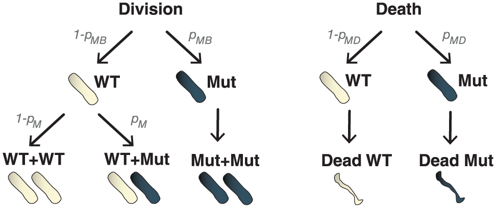
Possible outcomes for bacterial division and death events produced by the HF model. Division can occur in mutant bacteria (blue) with probability p_MB or WT bacteria (white) with probability (1 − p_MB). Division of WT bacteria can produce new WT bacteria with probability (1 − p_M) or mutant bacteria with probability p_M. Mutant bacteria produce new mutant bacteria. In this example, we therefore assume that the probability of a mutant reverting to WT is negligible. Death can occur in mutant bacteria with probability p_MD, or WT bacteria with probability (1 − p_MD), reducing the respective population by one. HF indicates high fidelity; WT, wild type.

For each event in the series of bacterial divisions and deaths produced by the HF model, an MF simulation calculates the probability of each of these scenarios. We define the probability of a mutant bacterium division (p_MB), the probability of a new mutation occurring (p_M), and the probability of a mutant bacterium dying (p_MD). The values of these probabilities can be based on the current state of the MF simulation or on a fixed parameter, depending on the system being studied. The MF simulations advance one event (division or death) at a time and for each event uses a random number generator to determine which scenario occurs in this instance of the MF analysis. That is, it determines whether a bacterial division increases the WT or mutant population and whether a bacterial death decreases the WT or mutant population (Figure 3). Therefore, each replication of the MF analysis represents one possible rare event trajectory for the population trajectory produced by the HF model. Multiple MF replications for each population trajectory then generate a rare event trajectory probability distribution over time. In this sense, the MF analysis provides additional information compared with the HF model results: where the HF model outcomes only produce one rare event trajectory for each population trajectory, the MF analysis can estimate the distribution of possible rare event trajectories for each population trajectory.

Figure 3.

Illustration of MF analysis: multiple MF replications for a single HF model population trajectory. The HF model population trajectory is a result of a series of bacterial divisions (+) and deaths (−). This series of events is used to generate multiple possible rare event trajectories. These trajectories are combined to construct probability distributions over time. HF indicates high fidelity; MF, medium fidelity.

LF Analysis

The LF analysis aims to determine rare event trajectory probability distributions for each HF model simulation over time. As in MF analysis, these distributions are based on the HF model–generated population trajectory (eg, a series of bacterial divisions and deaths). Unlike MF analysis, the LF analysis calculates the probability distributions without simulating individual rare event trajectories.

Our LF analysis considers each HF model simulation a Markov chain, where the possible states of the system are the number of rare events. Continuing our bacterial mutation example, the possible states of the system are the number of mutant bacteria in the population. Therefore, if the HF model population trajectory had N total bacteria, then the Markov chain has N + 1 possible states, it could have 0, 1, 2 . . . N mutant bacteria.

We use the same probabilities defined above for MF analysis: p_MB, p_M, and p_MD representing mutant bacterium division, new mutation, and mutant bacterium death, respectively, to quantify the transition probabilities between states of the Markov chain.

We define the probability of the Markov chain being in state X, p_X(i), as the probability of having X mutant bacteria after event i. We update p_X(i) over the series of division and death events from HF model simulations as follows.

When event i is a bacterial division,

p_{X} (i) = p_{X} (i - 1) (1 - p_{M}) (1 - p_{M B}) + p_{X - 1} (i - 1) [p_{M B} + (1 - p_{M B}) p_{M}]

(1)

This probability definition reflects all possible outcomes as illustrated in Figure 2. The first term in equation (1) represents the case where there were X mutant bacteria before event i, and no mutation or division of mutant bacteria occurred (Figure 4). The second term represents the case where there were X − 1 mutant bacteria before event i, and there was either a division of a mutant bacterium or a division of a WT bacterium and a mutation.

Figure 4.

Low-fidelity analysis: Markov chain representing progression of mutant bacterial population. Each circle represents a state of the Markov chain and arrows indicate transition probabilities between states. These transition probabilities are used to construct equations (1) and (2). Note that p_MB is 0 when X = 0.

When event i is a bacterial death event,

p_{X} (i) = p_{X} (i - 1) (1 - p_{M D}) + p_{X + 1} (i - 1) p_{M D}

(2)

The first term represents the case where there were X mutant bacteria before event i, and the death occurred in a WT bacterium. The second term represents the case where there were X + 1 mutant bacteria before event i, and the death occurred in a mutant bacterium. Iterative application of these transition probabilities for each bacterial division and death event produces an evolving probability distribution for the Markov chain.

These MF and LF approaches are easily adapted to analyze other stochastic HF models and rare events. MATLAB code implementing multifidelity analysis is available as supplementary material and described in the supplementary text. Next, we describe the application of multifidelity analysis in a test case.

Test Case Definition: Rare Antibiotic Resistance–Conferring Mutations in Mycobacterium tuberculosis

As a test case to validate multifidelity analysis and illustrate some of its applications, we consider the rare emergence of antibiotic resistance in the context of TB disease. Tuberculosis is caused by Mycobacterium tuberculosis and is characterized by the formation of granulomas in patient lungs. Granulomas are the site of infection for TB and contain bacteria, host cells, and dead cell debris. Mycobacterium tuberculosis can mutate to acquire resistance against various antibiotics, but these events are relatively rare at the bacterial scale (~10^–8 per cell division).^14–17 Nevertheless, drug-resistant TB is rising globally. Between 1% and 38% of new TB cases were drug resistant in 2016.¹⁸ It is vital to understand the emergence of drug-resistant bacteria in the context of granulomas if we are to minimize the emergence of resistance to new antibiotics and antibiotic regimens.^19,20 Although resistance is well-studied in bacterial cultures where population sizes easily reach 10,¹⁰ it is difficult to isolate and track-resistant bacteria within granulomas because animal models of TB disease are costly and every granuloma contains between 10² and 10⁶ bacteria.²¹

An HF stochastic computational model, GranSim, describing single granuloma formation and function has been applied to study various immune, bacterial, and antibiotic mechanisms within granulomas.^22–26 Although GranSim is more cost- and time-effective than animal studies of TB, it remains limited in its ability to evaluate rare resistance emergence at biologically relevant mutation rates. For example, if the probability of resistance per granuloma (based on mutation frequency and number of bacteria per granuloma) is 10⁻⁵, then it would require 100 000 simulations to obtain one granuloma containing a resistant bacterium. The computational time required for one iteration of this model is ~2 CPU hours on a high-performance computing cluster.²⁷ It would therefore require large computational resources to obtain a small number of representative granulomas containing resistant bacteria. Here, we apply multifidelity analysis to GranSim outputs to illustrate their utility in predicting low-frequency mutation events.

GranSim

GranSim is a hybrid, multiscale, agent-based model describing the spatial and temporal aspects of granuloma formation and function. The model tracks individual immune cells (macrophages and T cells), and bacteria, as well as cytokines and chemokines, and is calibrated to data from M tuberculosis–infected nonhuman primates. Biological mechanisms encompassed by GranSim are briefly reviewed here. A detailed model description along with parameter values, pseudocode, and a model executable are available online at http://malthus.micro.med.umich.edu/GranSim/. The model environment is a 2-dimensional grid representing a 4 mm × 4 mm section of lung tissue. Macrophage agents within GranSim can be in one of 3 states: resting, activated, or infected. Resting macrophages become activated in response to bacteria and/or cytokine signals (TNF-α and IFN-γ). Resting and activated macrophages are able to phagocytose and/or kill bacteria. If a macrophage phagocytoses a bacterium without killing it, the macrophage’s state changes to infected. T-cell agents within GranSim are classified based on function as regulatory T cells, effector T cells, or cytotoxic T cells. These T-cell agents produce various cytokines and chemokines including TNF-α, IFN-γ, IL-10, CCL2, CCL5, and CXCL9/10/11 and thereby regulate macrophage and T-cell responses to infection. Macrophage and T-cell agents move randomly on the simulation grid unless there are chemotactic signals in their environment in which case they migrate in the direction of the chemotactic molecule gradient. Bacterial agents grow and divide at a specified growth rate based on their location (intracellular, extracellular, or in caseum). These growth rates are based on in vitro experiments and calibrated to nonhuman primate data. On each division, bacteria are able to mutate to become drug resistant. Resistance in M tuberculosis is often associated with a fitness cost, which is incorporated in the model as a reduced growth rate.

Population trajectories obtained from GranSim, as in the illustrative example above, are the number of bacteria in a granuloma over time. In this case, the population trajectories reflect detailed immunological and microbiological interactions throughout 200 days of M tuberculosis infection within a single granuloma. GranSim outputs include the series of bacterial divisions and deaths that gave rise to each population trajectory. Furthermore, GranSim can produce rare event trajectories (in this case, the number of antibiotic-resistant bacteria over time) but would require an unrealistic number of simulations to analyze dynamics at biologically relevant mutation frequencies.²⁸ The GranSim data set used here was generated in previous work²⁹ and includes population trajectories for 348 simulated granulomas.

MF analysis of GranSim simulations

For MF analysis, we use the series of bacterial divisions and deaths from each simulation of GranSim as events in the Monte Carlo simulation. We calculate the probability of a mutant bacterium division (p_MB), the probability of a new mutation occurring (p_M), and the probability of a mutant bacterium dying (p_MD) based on biological measurements as well as the current state of the MF analysis simulation at each time point.

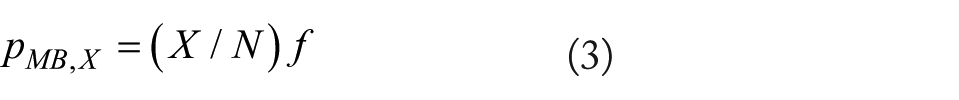
We define p_MB to take into account the number of resistant bacteria currently in the simulation (X), the total number of bacteria in the population (N), as well as the replicative fitness (f) of resistant bacteria relative to WT bacteria. We define 0 < f < 1, eg, f = 0.8 implies a fitness cost of 20% reduction in growth rate incurred for resistance acquisition. Therefore, we define p_MB,X, the probability of a mutant bacterium division given X mutant bacteria currently in the simulation as follows:

p_{M B, X} = (X / N) f

(3)

If the division was not a resistant bacterium, we define the probability of acquiring a new resistance-conferring mutation (p_M) as the product of the per-generation mutation probability (p_M), and the number of resistance-conferring mutations for the antibiotic of interest. When the event is a bacterial death, we define p_MD,_X as the probability of the bacterial death being a resistant bacterium, given X-resistant bacteria in the current simulation:

p_{M D, X} = X / N

(4)

For each population trajectory, we simulate 50 000 MF analysis replications. This allows the prediction of rare events at much lower frequencies than the HF model, but there remains a limit on how many MF analysis replications are feasible.

LF analysis of GranSim simulations

For LF analysis of GranSim, we define the probability for a given state of the Markov chain as described above (equations (1) and (2)), with p_MB and p_MD defined to depend on X and N, as for the MF analysis (equations (3) and (4)). This system is therefore a time-varying Markov chain as the transition probabilities between states vary over time as N changes. The LF analysis has no lower limit on the frequencies it can evaluate because individual rare event trajectories are not being generated.

Multifidelity analysis assumptions

While some mechanistic details of the host-pathogen interactions within granulomas are captured in multifidelity analysis parameters (eg, the relative fitness of resistant bacteria), others cannot be included. Multifidelity analysis implicitly makes the following simplifying assumptions.

The MF and LF analyses cannot track individual bacteria and their varying generation times based on their location within granulomas (eg, intracellular vs extracellular). The per-generation mutation probability (p_M) for M tuberculosis is known to increase with increasing generation time.²⁸ Our multifidelity analysis therefore assumes an average generation time for all bacteria.

The current multifidelity analysis methods do not account for the delay between divisions of the same bacterium. That is, based on the probability definitions in equations (3) and (4), the same bacterium can divide twice in consecutive model time steps, which is not biologically accurate. Below, we compare HF model results with multifidelity analysis predictions to validate the method and to illustrate that these assumptions do not significantly affect our predictions in the TB test case.

Validation in Test Case: Multifidelity Analysis Recapitulates HF Model Rare Event Dynamics

To validate multifidelity analysis, we compare their rare event predictions with observed values in the HF model (GranSim) at high mutation frequency. The average population trajectory for GranSim is included in Figure 5A. First, we compare multifidelity analysis–predicted probability of having at least one resistant bacterium with the observed fraction of HF model granulomas with at least one resistant bacterium (Figure 5B). Second, we compare the probability distributions for the number of resistant bacteria after 200 days of infection (Figure 5C). For both of these metrics, MF and LF predictions are nearly identical, and most of the observed HF model data fall within 1 standard deviation of the MF and LF predictions. Comparing HF model–observed and MF analysis–predicted resistance trajectories (rare event trajectories) for representative granulomas shows similar patterns of sporadic resistance emergence followed by periods of no resistance (Figure 5D). The average period of resistance (time between emergence of new resistance and elimination of that resistant population) is 11.5 days for HF model and 11.7 days for MF analysis (Figure 5E). Figure 5 illustrates that similar information can be obtained from MF or LF analysis (Figure 5B and C) and demonstrates the additional information available from MF analysis (Figure 5D and E). Taken together, these results illustrate that multifidelity analysis is able to predict both dynamics and probability distributions of rare event trajectories in the HF model.

Figure 5.

Multifidelity analysis validation against HF model results. Each panel shows observed values from HF model simulation at high mutation frequencies (2 × 10⁻⁸ per 10-minute HF model time step), along with MF and LF predictions at these frequencies. (A) The average population trajectory produced by the HF model shows early increase in bacterial numbers, followed by a steep decline induced by adaptive immunity, and subsequent stable bacterial numbers. Solid lines show means, dotted lines show ±standard deviations. Note that the lower standard deviation dotted line cannot be displayed on log-scale for the entire simulation period. (B) Probability of resistance per granuloma. Note that curves for MF and LF analyses overlap. HF model curve shows the fraction of granulomas with at least one resistant bacterium. (C) Distribution of number of resistant bacteria per granuloma. In panels B and C, HF model results have a single value because the fraction is calculated out of the 348 granulomas studied. MF and LF results show mean and standard deviations because these analyses predict a resistance probability for each individual granuloma, which we average to compare with HF model results. (D) Number of resistant bacteria per granuloma over time for 10 illustrative examples of HF model and MF analysis (this information is not available from the LF analysis). (E) Distributions for the number of days that resistant bacteria remain within individual granulomas (resistance period) for all HF model granuloma simulations and for 10 illustrative replications of MF analysis for each granuloma. HF indicates high fidelity; LF, low fidelity; MF, medium fidelity.

Table 1 shows computational times recorded for the HF model, MF, and LF analyses. While implementation of multifidelity analysis in other models would have different computational times depending on the number of events being simulated, this test case illustrates the potential computational savings in studying rare events with multifidelity analysis. We next apply multifidelity analysis to illustrate how it can be leveraged to analyze rare events with reduced computational cost.

Table 1.

Simulation time for HF model, MF analysis, and LF analysis.

	Simulation time
GranSim	107 ± 14 minutes (single replication)
MF analysis	81 ± 14 minutes (50 000 replications)
LF analysis	4 ± 1 seconds

Abbreviations: HF, high fidelity; LF, low fidelity; MF, medium fidelity.

Predictions in Test Case

MF and LF analyses enable sensitivity analysis at biologically relevant mutation frequencies

One challenge in using HF models is to quantify model sensitivity to parameters when the model outputs of interest are rare events, eg, the emergence of resistance in TB granulomas. Here, we illustrate how multifidelity analysis can be used to perform sensitivity analysis (SA) in biologically relevant mutation frequency ranges. For the TB test case, some model outputs of interest are the probability of resistance per granuloma, the expected number of resistant bacteria per granuloma, and the average resistance period. The model parameters we vary in this SA are mutation frequency (p_M) and relative fitness (f).

Both the probability of resistance per granuloma (Figure 6A) and the expected number of resistant bacteria (Figure 6B) appear to correlate more strongly with mutation frequency than relative fitness, where relative fitness has a stronger effect on the resistance period (Figure 6C). Indeed, partial correlations between parameters and each of the model outputs indicate that mutation frequency is the main driver of the expected number of resistant bacteria (Table 2). Although both mutation frequency and relative fitness significantly contribute to the probability of resistance and the resistance period, relative fitness has a stronger correlation with the resistance period than with the probability of resistance. This indicates that a higher relative fitness of a resistant strain allows that strain to persist in the granuloma for longer, whereas a higher mutation frequency will allow more new mutations to occur, both of which result in higher probability of resistance per granuloma. Multifidelity analysis predicts that similar parameter influences are at play at high and low mutation frequencies.

Figure 6.

MF analysis–predicted effect of relative fitness (x-axes) and mutation frequency (y-axes) on (A) the probability of resistance per granuloma after 200 days of infection, (B) expected number of resistant bacteria per granuloma after 200 days of infection, and (C) average length of resistance periods (days). Note that probability of resistance per granuloma and the expected number of resistant bacteria per granuloma, but not the resistance period, are outputs that can also be assessed with LF analysis (Supplement Figure S1). Coefficients of variation corresponding to Figure 6 and Figure S1 panels are included in Figure S2. The ranges used for relative fitness and mutation frequency values are informed by experimental measurements in vitro and in nonhuman primates infected with Mycobacterium tuberculosis and chosen to be able to illustrate the application of the multifidelity analysis. Mutation frequency is varied between 2 × 10⁻¹² and 2 × 10⁻⁸ per 10-minute HF model time step, spanning the values between the experimentally measured frequency (2 × 10⁻¹²)²⁸ and the frequency used in the HF simulations used for validation above (2 × 10⁻⁸). Relative fitness is varied between 0 and 1 to capture the breadth of possible fitness cost influences. Relative fitness estimates for key anti-TB drugs are 0.8 to 0.9.^30-32 HF indicates high fidelity; MF, medium fidelity; TB, tuberculosis.

Table 2.

Sensitivity analysis results.

		Model outputs
		Probability of resistance	Expected no. of resistant bacteria	Resistance period
Parameters	Mutation frequency	.86 (6 × 10⁻⁸)	.46 (.02)	.88 (2 × 10⁻⁸)
	Relative fitness	.43 (.03)	.36 (.08)	.96 (3 × 10⁻¹³)

Partial correlation coefficients (P values) are shown for combinations of model parameters and outputs.

These parameter influences can be contextualized for TB in terms of different M tuberculosis lineages. Experimental work has found that lineage 2 strains of M tuberculosis have a 4-fold higher mutation frequency than lineage 4 strains.³³ Furthermore, resistant bacteria of the Beijing strain (part of lineage 2) were found to have higher relative fitness compared with non-Beijing strains.³⁴ Taken together with our predictions, this would suggest that lineage 2 strains not only develop new resistance more often but that these resistant bacteria also remain within granulomas for longer, possibly allowing opportunity for further mutation to acquire multidrug resistance and compensatory mutations. Indeed, the Beijing strain has been associated with multidrug-resistant TB.^35,36

Multifidelity analysis can discern influence of stochastic events and parameter fluctuations

If stochasticity in the system is strong enough to mask parameter effects, it could affect our ability to predict rare events in the system. In the TB test case, we know the mutation frequency, but the timing of mutations is entirely random. Being able to predict the most dangerous times for mutations to occur could inform public health policy related to diagnosis and case-finding strategies. We therefore apply multifidelity analysis to ask, “what is the influence of the timing of mutations (a stochastic event) vs the influence of relative fitness or mutation frequency (model parameters)?”

We incorporate the timing of mutations into MF and LF analyses by manipulating the initial distribution of resistant bacteria and varying the starting time of the analyses. In other words, we assume that there is exactly 1 resistant bacterium at various times of each HF model simulation (5, 15, 30, 50, and 100 days after infection) and then predict the rare event trajectories and probability distributions over the rest of the infection (up to 200 days). Therefore, we ask whether there is one mutation at days 5, 15, 30, 50, or 100; what is the probability of resistance after 200 days of infection; and how does the timing of the initial mutation affect this probability.

For low relative fitness values, the timing of the first mutation has little influence because the presence of resistant bacteria after 200 days will almost entirely depend on new mutations (Figure 7A and C). In contrast, at high relative fitness, a nonmonotonic relationship emerges between the timing of the first mutation and the probability of resistance after 200 days of infection (Figure 7B and D). Although the nonmonotonic relationship is evident for both high and low mutation frequencies, the relative influence of timing is larger at lower mutation frequencies. At low mutation frequencies, the probability of resistance after 200 days decreases by 99% (from .13 to 6 × 10⁻⁴) if the first mutation occurs at 5 days compared with 30 days after infection, respectively. At high mutation frequencies, the probability of resistance decreases by 33% (from .3 to .2). The influence of timing in this case relates to the population trajectories of the HF model (Figure 5A). A mutation at 30 days after infection would occur immediately prior to a large contraction in the bacterial population, making it unlikely that this mutant bacterium will survive. Taken together, these results illustrate how MF and LF analyses can be applied to extrapolate HF model predictions to lower frequencies.

Figure 7.

Effect of relative fitness, mutation frequency, and timing (in days) of the first mutation on the probability of resistance after 200 days of infection. Mutation frequencies of 2 × 10⁻⁸ (A, B) and 2 × 10⁻¹² (C, D) per 10-minute HF model time step are considered along with relative fitness values of 0.25 (A, C) and 1 (B, D). Results are shown for MF analysis predictions, but LF analysis predictions are nearly identical (Supplement Figure S3). Bars represent mean probabilities more than 348 simulations and error bars represent standard error of the mean. Stars indicate statistically significant differences (P < .0005) as determined through 1-way ANOVA and Scheffé’s multiple comparison procedure. ANOVA indicates analysis of variance; HF, high fidelity; MF, medium fidelity.

Discussion

Rare events can be challenging to study in complex biological systems, either experimentally or computationally. We outline a multifidelity analysis approach that can be applied to compute probability distributions of rare events over time. Our analysis method takes as input a series of discrete population-level events generated by an HF computational model of the biological system. This series of events provides input for MF and LF analyses to predict the probability and dynamics of rare events for each series of events (ie, each simulation of the HF model). We show that MF and LF analyses can accurately predict HF model results at high frequencies and illustrate how they can be applied to analyze results obtained from HF model simulations.

Multifidelity analysis could be applied as an intermediate step toward more sophisticated approaches such as accelerating HF model simulation or construction of multifidelity models.^2,4,8 For example, MF and LF predictions could be used to identify specific time frames to focus on during weighted ensemble simulations or to isolate certain model mechanisms that are important to maintain when constructing multifidelity models.

The multifidelity analysis presented here was performed separately from the HF model, using data from previous simulations of the HF model. However, it should be noted that both MF and LF analyses can be integrated with the HF model so that the rare event trajectories and probability distributions are updated in real time following each discrete event as the HF model simulation is running. Integrating MF analysis with the HF model simulation would be costlier than LF analysis as multiple replications would be performed for each update. Such an integrated approach would be valuable if large amounts of high time resolution data need to be stored in order for multifidelity analysis to be performed separately and if multifidelity analysis parameter values do not need to be varied.

Multifidelity analysis could also be applied to experimental data. As the tools for single-cell analysis become more sophisticated and accessible, experimentally obtained single-cell data could be used to generate the series of discrete events required for multifidelity analysis. For example, bacterial growth in microfluidic devices has been used to carefully monitor bacterial division and death at the single-cell level.^37,38 These data could be used as input for multifidelity analysis, thereby predicting possible rare event trajectories for experimental data. Transition probabilities could be based on other measurements in the system at the same time (eg, gene expression data³⁹) or from other experimental systems (eg, mutation frequency in animal models²⁸). In this way, multifidelity analysis could inform iterative experimental design (eg, time points, number of replications) without the construction of an HF model or could bridge single-cell and batch culture results (eg, how does a certain mutation frequency drives resistance at the single-cell level over time?).

In summary, as the sophistication of computational and experimental models advances, strategic and stepwise analysis of the vast amounts of data they produce will become important to maximize the amount of knowledge extracted from these data. We believe that multifidelity analysis could provide one such approach.

Supplemental Material

2018-06-11-Pienaar-SupplementaryText – Supplemental material for Multifidelity Analysis for Predicting Rare Events in Stochastic Computational Models of Complex Biological Systems

Supplemental material, 2018-06-11-Pienaar-SupplementaryText for Multifidelity Analysis for Predicting Rare Events in Stochastic Computational Models of Complex Biological Systems by Elsje Pienaar in Biomedical Engineering and Computational Biology

Footnotes

Acknowledgements

Medium-fidelity analysis simulations were performed on resources at the Rosen Center for Advanced Computing at Purdue University. I thank Drs. Denise Kirschner and Jennifer Linderman for early reviews of the manuscript.

Funding:

The author(s) disclosed receipt of the following financial support for the research, authorship, and/or publication of this article: The author thanks the Kirschner and Linderman Labs at the University of Michigan for use of GranSim data supported by the following NIH grants: U01HL131072 and R01 HL 110811. GranSim data also used resources of the National Energy Research Scientific Computing Center, which is supported by the Office of Science of the US Department of Energy under contract no. DE-AC02-05CH11231 and the Extreme Science and Engineering Discovery Environment (XSEDE), which is supported by National Science Foundation grant number MCB140228.

Declaration of conflicting interests:

The author(s) declared no potential conflicts of interest with respect to the research, authorship, and/or publication of this article.

Author Contributions

EP designed the approach, acquired and analyzed the data and drafted the article.

Supplemental Material

Supplementary material for this article is available online.

References

Donovan

Tapia

Sullivan

et al . Unbiased rare event sampling in spatial stochastic systems biology models using a weighted ensemble of trajectories. PLoS Comput Biol. 2016;12:e1004611.

Forrester

AIJ

Sóbester

Keane

. Multi-fidelity optimization via surrogate modelling. P Roy Soc A-Math Phy. 2007;463:3251-3269.

Sandmann

. Rare event simulation methodologies in systems biology. In: Rubino

Tuffin

, eds. Rare Event Simulation Using Monte Carlo Methods. Chichester, UK: John Wiley & Sons Ltd; 2009:243-266.

Liu

Koziel

Zhang

A multi-fidelity surrogate-model-assisted evolutionary algorithm for computationally expensive optimization problems. J Comput Sci. 2016;12:28-37.

Bazzi

Blasques

Koopman

Lucas

Time-varying transition probabilities for Markov regime switching models. J Time Series Anal. 2017;38:458-478.

Kirschner

Hunt

Marino

Fallahi-Sichani

Linderman

JJ.

Tuneable resolution as a systems biology approach for multi-scale, multi-compartment computational models. Wiley Interdiscip Rev Syst Biol Med. 2014;6:289-309.

Mamonov

Lettieri

Ding

et al . Tunable, mixed-resolution modeling using library-based Monte Carlo and graphics processing units. J Chem Theory Comput. 2012;8:2921-2929.

Choi

Seo

K-M

Kim

GT.

Accelerated simulation of discrete event dynamic systems via a multi-fidelity modeling framework. Appl Sci. 2017;7:1056.

Pienaar

Matern

Linderman

Bader

Kirschner

DE.

Multiscale model of Mycobacterium tuberculosis infection maps metabolite and gene perturbations to granuloma sterilization predictions. Infect Immun. 2016;84:1650-1669.

10.

Jayathilake

Gupta

et al . A mechanistic individual-based model of microbial communities. PLoS ONE. 2017;12:e0181965.

11.

Harcombe

Riehl

Dukovski

et al . Metabolic resource allocation in individual microbes determines ecosystem interactions and spatial dynamics. Cell Rep. 2014;7:1104-1115.

12.

Harrigan

Sultan

Hernandez

et al . MSMBuilder: statistical models for biomolecular dynamics. Biophys J. 2017;112:10-15.

13.

Suarez

Adelman

Zuckerman

DM.

Accurate estimation of protein folding and unfolding times: beyond Markov state models. J Chem Theory Comput. 2016;12:3473-3481.

14.

David

HL.

Probability distribution of drug-resistant mutants in unselected populations of Mycobacterium tuberculosis. Appl Microbiol. 1970;20:810-814.

15.

Boshoff

Reed

Barry

III Mizrahi

DNAE2 polymerase contributes to in vivo survival and the emergence of drug resistance in Mycobacterium tuberculosis. Cell. 2003;113:183-193.

16.

Werngren

Hoffner

SE.

Drug-susceptible Mycobacterium tuberculosis Beijing genotype does not develop mutation-conferred resistance to rifampin at an elevated rate. J Clin Microbiol. 2003;41:1520-1524.

17.

McGrath

van Pittius

NCG

van Helden

Warren

Warner

DF.

Mutation rate and the emergence of drug resistance in Mycobacterium tuberculosis. J Antimicrob Chemother. 2014;69:292-302.

18.

WHO. Global tuberculosis report 2017. Geneva, Switzerland: WHO; 2017.

19.

Dartois

The path of anti-tuberculosis drugs: from blood to lesions to mycobacterial cells. Nat Rev Microbiol. 2014;12:159-167.

20.

Pienaar

Dartois

Linderman

Kirschner

In silico evaluation and exploration of antibiotic tuberculosis treatment regimens. BMC Syst Biol. 2015;9:79.

21.

Lin

Ford

Coleman

et al . Sterilization of granulomas is common in active and latent tuberculosis despite within-host variability in bacterial killing. Nat Med. 2014;20:75-79.

22.

Cilfone

Perry

Kirschner

Linderman

JJ.

Multi-scale modeling predicts a balance of tumor necrosis factor-α and interleukin-10 controls the granuloma environment during Mycobacterium tuberculosis infection. PLoS ONE. 2013;8:e68680.

23.

Fallahi-Sichani

El-Kebir

Marino

Kirschner

Linderman

JJ.

Multiscale computational modeling reveals a critical role for TNF-α receptor 1 dynamics in tuberculosis granuloma formation. J Immunol. 2011;186:3472-3483.

24.

Pienaar

Cilfone

Lin

et al . A computational tool integrating host immunity with antibiotic dynamics to study tuberculosis treatment. J Theor Biol. 2015;367:166-179.

25.

Ray

Flynn

Kirschner

DE.

Synergy between individual TNF-dependent functions determines granuloma performance for controlling Mycobacterium tuberculosis infection. J Immunol. 2009;182:3706-3717.

26.

Segovia-Juarez

Ganguli

Kirschner

. Identifying control mechanisms of granuloma formation during M. tuberculosis infection using an agent-based model. J Theor Biol. 2004;231:357-376.

27.

Pienaar

Sarathy

Prideaux

et al . Comparing efficacies of moxifloxacin, levofloxacin and gatifloxacin in tuberculosis granulomas using a multi-scale systems pharmacology approach. PLoS Comput Biol. 2017;13:e1005650.

28.

Ford

Lin

Chase

et al . Use of whole genome sequencing to estimate the mutation rate of Mycobacterium tuberculosis during latent infection. Nat Genet. 2011;43:482-486.

29.

Pienaar

Linderman

Kirschner

DE.

Emergence and selection of isoniazid and rifampin resistance in tuberculosis granulomas. PLoS ONE. 2018;13:e0196322.

30.

Trauner

Borrell

Reither

Gagneux

Evolution of drug resistance in tuberculosis: recent progress and implications for diagnosis and therapy. Drugs. 2014;74:1063-1072.

31.

Davies

Billington

Bannister

Weir

McHugh

Gillespie

SH.

Comparison of fitness of two isolates of Mycobacterium tuberculosis, one of which had developed multi-drug resistance during the course of treatment. J Infect. 2000;41:184-187.

32.

Gagneux

Fitness cost of drug resistance in Mycobacterium tuberculosis. Clin Microbiol Infect. 2009;15:66-68.

33.

Ford

Shah

Maeda

et al . Mycobacterium tuberculosis mutation rate estimates from different lineages predict substantial differences in the emergence of drug-resistant tuberculosis. Nat Genet. 2013;45:784-790.

34.

Toungoussova

Caugant

Sandven

Mariandyshev

Bjune

Impact of drug resistance on fitness of Mycobacterium tuberculosis strains of the W-Beijing genotype. FEMS Immunol Med Microbiol. 2004;42:281-290.

35.

Buu

Huyen

Lan

et al . The Beijing genotype is associated with young age and multidrug-resistant tuberculosis in rural Vietnam. Int J Tuberc Lung Dis. 2009;13:900-906.

36.

Zhou

van den Hof

Wang

et al . Association between genotype and drug resistance profiles of Mycobacterium tuberculosis strains circulating in China in a national drug resistance survey. PLoS ONE. 2017;12:e0174197.

37.

Manina

Dhar

McKinney

JD.

Stress and host immunity amplify Mycobacterium tuberculosis phenotypic heterogeneity and induce nongrowing metabolically active forms. Cell Host Microbe. 2015;17:32-46.

38.

Aldridge

Fernandez-Suarez

Heller

et al . Asymmetry and aging of mycobacterial cells lead to variable growth and antibiotic susceptibility. Science. 2012;335:100-104.

39.

Wakamoto

Dhar

Chait

et al . Dynamic persistence of antibiotic-stressed mycobacteria. Science. 2013;339:91-95.

Supplementary Material

Please find the following supplemental material available below.

For Open Access articles published under a Creative Commons License, all supplemental material carries the same license as the article it is associated with.

For non-Open Access articles published, all supplemental material carries a non-exclusive license, and permission requests for re-use of supplemental material or any part of supplemental material shall be sent directly to the copyright owner as specified in the copyright notice associated with the article.

0.00 MB

0.77 MB