Sage Journals: Discover world-class research

Abstract

Atrazine, a triazine-class herbicide widely used in U.S. Corn and soybean production is highly soluble, persistent and prone to runoff. It poses risks such as reduced aquatic productivity and biological endocrine disruption. Observation-driven geostatistical models can extend sparse monitoring networks by estimating contaminant levels across space and time. We evaluated all available Iowa surface water atrazine measurements from 1986 to 2025 (n = 13,247), identifying sparse and inconsistent sampling before 2000 and after 2004, with a period of sustained high sampling intensity from 2000 to 2004 (>1,000 samples per year). In this study, we applied a geostatistical, Bayesian Maximum Entropy (BME) framework to model log-transformed atrazine concentrations in Iowa surface waters from 2000 to 2004 using 6,478 observations from 673 monitoring sites. We compared a traditional spatial-only geostatistical framework with a fully spatiotemporal BME model incorporating both spatial and temporal data. Spatiotemporal dependence was modeled using an additive, nested space–time, exponential covariance structure. This allows spatial and temporal autocorrelation to jointly inform prediction while preserving localized contamination patterns. Model performance was evaluated using leave-one-out cross-validation. Results show spatiotemporal BME significantly outperformed spatial-only approaches, improving predictive power (R² = 0.73 vs. 0.64) and reducing mean squared error (0.318 vs. 0.432) log µg²/L. Performance gains were largest for error metrics sensitive to extreme values, with spatiotemporal BME substantially reducing mean squared error relative to spatial-only models, indicating improved representation of episodic high-concentration events. Our findings demonstrate atrazine exposure risk appears to be predictable and likely aligned with seasonal application, chemical half-life, and delayed runoff. These processes likely produce localized hotspots often exceeding the U.S. EPA’s 3 µg/L drinking water standard. Atrazine correlation showed strong spatial (mobility 25–150 km) and temporal persistence (~20–50 days). This approach complements mechanistic models, offering a flexible, data-driven framework for environmental health monitoring where data are sparse or irregular.

Keywords

atrazine surface water contamination spatiotemporal modeling geostatistics covariance modeling water quality prediction pesticide monitoring environmental exposure assessment

Background

Atrazine, a triazine herbicide introduced in the 1950s, is widely used for pre-emergence weed control in corn, sorghum, and sugarcane (Agency for Toxic Substances and Disease Registry, 2025; Sass & Colangelo, 2006). It remains among the most heavily applied herbicides in the U.S., with approximately 70 million pounds used annually (U.S. Environmental Protection Agency, 2025; U.S. Geological Survey, 2025b). Although banned in the European Union due to environmental and health concerns (Chavez Rodriguez et al., 2021; Sass & Colangelo, 2006), atrazine remains common in U.S. agriculture because of its effectiveness and low cost. Its high solubility and extensive use contribute to widespread environmental detection, particularly in surface waters, with concentrations varying by geography, crop practices, and weather (Chavez Rodriguez et al., 2021; U.S. Geological Survey, 2025a). The highest levels occur in the Midwest, where intensive corn and soybean cultivation drive runoff (U.S. Geological Survey, 2025a).

Atrazine-related risks to ecosystems and public health have been documented for decades, including reproductive and developmental effects on aquatic organisms and terrestrial wildlife (U.S. Environmental Protection Agency, 2025; Center for Biological Diversity, 2025). In aquatic systems, these effects are driven in part by inhibition of photosynthesis in plants through photosystem II blockade. This reduction in primary productivity contributes to lower oxygen levels, reduced biodiversity, and food web instability. (Agency for Toxic Substances and Disease Registry, 2025; Center for Biological Diversity, 2025; Chavez Rodriguez et al., 2021; Sass & Colangelo, 2006; U.S. Geological Survey, 2025a).

Atrazine has also been documented to disrupt endocrine systems causing reproductive, developmental, and immune abnormalities across taxa (Agency for Toxic Substances and Disease Registry, 2025; Sass & Colangelo, 2006). Amphibians are especially sensitive as laboratory and field studies have linked even low concentrations to feminization and hermaphroditism in male frogs (Agency for Toxic Substances and Disease Registry, 2025; Center for Biological Diversity, 2025; Sass & Colangelo, 2006; U.S. Geological Survey, 2025a). Epidemiological studies link atrazine in drinking water to human endocrine disruption and elevated risks of hormonal imbalances, birth defects, cancers, shorter pregnancies, and altered menstrual cycles (U.S. Environmental Protection Agency, 2025; Agency for Toxic Substances and Disease Registry, 2025; Center for Biological Diversity, 2025; Chavez Rodriguez et al., 2021; Lerro et al., 2017; Roh et al., 2023; Sass & Colangelo, 2006). For regulatory context, the U.S. EPA sets an aquatic plant concentration–equivalent level of concern (CE-LOC) of 9.7 µg/L, defined as a 60-day average exposure threshold (U.S. Environmental Protection Agency, 2025). The EPA also sets a drinking water maximum contaminant level (MCL) of 3 µg/L (U.S. Environmental Protection Agency, 2025; U.S. Geological Survey, 2025a).

Observation-driven geostatistical models provide a cost-effective means of extending spatial and temporal coverage from limited monitoring data (G. Christakos, 1990; M. L. Serre & Christakos, 1999). These models leverage spatial autocorrelation to estimate values at unsampled locations (Cliff & Ord, 1981). Developed originally for mining, geostatistics became widely used in data-scarce decision settings (G. Christakos, 1998; Isaaks & Srivastava, 1989). They provide a formal framework for uncertainty reduction across applications such as reservoir characterization, public health, and large-scale environmental estimation (G. Christakos, 1990; G. Christakos et al., 2001). These approaches have also been applied to water quality prediction due to their ability to generate accurate estimates with relatively low computational demand (Delhomme, 1978; Isaak et al., 2014; Jat & Serre, 2018; LoBuglio et al., 2007; Peterson & Urquhart, 2006).

Traditional geostatistical models generally do not incorporate temporal autocorrelation limiting their utility for persistent contaminants like atrazine. Spatiotemporal approaches accounting for both spatial and temporal dependence have been shown to improve predictive accuracy (Bogaert et al., 2009; G. Christakos & Serre, 2000; de Nazelle et al., 2010; Xu et al., 2016). However, none have been applied to atrazine in surface waters (Chavez Rodriguez et al., 2021; Roh et al., 2023). Given atrazine’s persistence and strong temporal structure, this study evaluates both spatial-only and space–time models to estimate atrazine concentrations in Iowa streams. The goal is to quantify added value of including temporal autocorrelation into the estimation matrix.

Although our dataset spans 2000 to 2004, it represents one of the last systematically collected, high-quality monitoring efforts for atrazine in U.S. surface waters (Iowa Department of Natural Resources, 2025; U.S. Geological Survey, 2025a, 2025b). State and national reporting has since declined. The U.S. Geological Survey ended the Pesticide National Synthesis Project after 2019, and USDA’s herbicide application surveys ceased regular updates after 2021 (U.S. Department of Agriculture, National Agricultural Statistics Service, 2022; U.S. Environmental Protection Agency, 2025; U.S. Geological Survey, 2025b). Surveillance in Iowa also dropped sharply after 2004. Despite these reductions, analyses indicate atrazine application rates have remained stable at 70 to 80 million pounds per year (U.S. Environmental Protection Agency, 2025; Sass & Colangelo, 2006; U.S. Geological Survey, 2025b), with geographic patterns through 2019 showing broadly consistent spatial distributions (U.S. Geological Survey, 2025b; U.S. Environmental Protection Agency, 2025). As a result, the 2000 to 2004 dataset remains informative for understanding the spatiotemporal structure and likely hotspots of atrazine contamination under stable application patterns (Iowa Department of Natural Resources, 2025; U.S. Environmental Protection Agency, 2025; U.S. Geological Survey, 2025a).

Methods

Data

This study focused on atrazine concentrations in Iowa surface waters collected between 2000 and 2004, which represents the most complete and consistently sampled interval in the statewide monitoring record. Spatiotemporal atrazine concentration data were obtained from the Iowa Department of Natural Resources (IDNR) and reported in micrograms per liter (µg/L). To identify the appropriate analysis window, we examined all available surface water atrazine measurements from Iowa’s state monitoring program spanning 1986 to 2025 (Iowa Department of Natural Resources, 2025; samples = 13,247).

Based on this review, analyses were restricted to 2000 to 2004, yielding a refined dataset of 6,478 measurements from 673 monitoring sites across 800 time points (Iowa Department of Natural Resources, 2025). Atrazine concentrations were analyzed on the log₁₀ scale to reduce right skewness and stabilize variance, as the distribution contained many observations clustered at near low concentrations. Throughout the manuscript, “log” denotes log₁₀. Measurements below the analytical limit of detection (LOD = 0.01 µg/L) were substituted with one-half the detection limit (0.005 µg/L) prior to transformation to permit inclusion of non-detects and avoid undefined log values. To represent the hydrological framework for analysis, we obtained medium-resolution flowline data for Iowa from the U.S. Geological Survey’s National Hydrography Dataset (U.S. Geological Survey, 2025a). These flowlines were used to represent streams and rivers across the state and to support spatial visualization of observed and predicted atrazine concentrations (U.S. Geological Survey, 2025b).

Analysis Strategy

We applied Bayesian Maximum Entropy (BME), an advanced space–time geostatistical framework that extends traditional kriging to estimate atrazine log-concentrations along Iowa’s stream network. BME applies space–time random field (S/TRF) theory to minimize mean squared error (MSE) and provide the Best Linear Unbiased Predictor (BLUP; G. Christakos, 1990; M. L. Serre & Christakos, 1999). BME has been widely applied in public health and environmental research (Abbott et al., 2025; G. Christakos, 1998; G. Christakos et al., 2001; de Nazelle et al., 2010; L. Fox et al., 2015, 2023, 2024; Reyes & Serre, 2014; Xu et al., 2016), including water quality studies to generate continuous surfaces of exposure (Jat & Serre, 2016, 2018; Messier et al., 2012, 2015; Valencia et al., 2023). Its mathematical foundations are described extensively in prior work (G. Christakos, 1990; G. Christakos & Serre, 2000; He & Christakos, 2023; M. L. Serre & Christakos, 1999).

BME kriging proceeds in three main steps. First, atrazine concentrations are treated as values observed at specific space–time coordinates, and the space–time random field characterizes the distribution of possible values at unsampled locations and times. A S/TRF can be written as $X (p)$ , where $p = (s, t)$ is a space/time point, $s$ is the spatial coordinate along the stream network and $t$ is time. The covariance function of the atrazine log-concentration is modeled by first calculating experimental covariance values, cˆ_X based on the measurement data, $x_{d} = [x_{1}, \dots, x_{n}]$ , and a covariance model is fit to it, $c_{x} (p, p') = E [(X (p) - m_{x} (p)) (X (p') - m_{x} (p'))]$ , where E[.] denotes the statistical expectation (expected value) and m_x is the S/TRF’s mean.

Covariance models characterize how atrazine concentrations vary across space and time (He & Christakos, 2023; M. L. Serre & Christakos, 1999). Spatial covariance describes the degree of similarity between monitoring sites as a function of distance, with the autocorrelation range marking the point beyond which observations are effectively independent (Cliff & Ord, 1981; Isaaks & Srivastava, 1989). This structure determines the influence of neighboring observations on predictions, consistent with Tobler’s First Law of Geography (G. Christakos, 1990; Isaaks & Srivastava, 1989).

We evaluated covariance based two models in this study: a spatial-only framework and a spatiotemporal (space-time) framework. The space–time covariance model we use is additive and separable, with the spatial and temporal components computed and evaluated independently. Euclidean spatial covariance models, such as the ones used in this study are a function of the straight-line distance between points, i.e. cˆ_XS $(d_{E}) = c_{1} (d_{E} (s, s'))$ , where $d_{E} (s, s')$ is the Euclidean distance between locations s and s′ , and $c_{1} (.)$ can be any permissible covariance model (Jat & Serre, 2016, 2018). For temporal covariance, cˆ_X is a function of time lag, $τ = t - t'$ . The full exponential based covariance model incorporating both space and time is written as, $c_{x} ((s, t), (s', t')) = c_{0} e x p (- 3 d (s, s') / a_{r}) e x p (- 3 | t - t' | / a_{t})$ where $c_{0}$ , a_r and a_t are the variance, spatial covariance range, and temporal covariance range (G. Christakos, 1990, 1998; M. L. Serre & Christakos, 1999).

The final step of the BME analysis is the integration stage, where the prior probability density function (PDF), defined by the covariance structure of atrazine concentrations, is updated using Bayesian conditionalization (G. Christakos, 1990; G. Christakos & Serre, 2000; M. L. Serre & Christakos, 1999). In practical terms, the covariance model (step 2) defines the spatial and temporal ranges over which atrazine concentrations are correlated and determines how strongly nearby observations influence predictions. In step 3, this covariance structure is combined with local observations to generate predicted values at unsampled locations and times. This generates spatiotemporal estimates of atrazine concentrations, which are mapped as continuous surfaces of predicted water quality across Iowa (L. Fox et al., 2023; Jat & Serre, 2016, 2018; Reyes & Serre, 2014). Following BME estimation, predicted concentrations were back-transformed to the original concentration scale, and results unless noted otherwise are reported in µg/L.

Observed atrazine concentrations were used as the sole inputs to the BME framework, from which spatial and spatiotemporal concentration estimates were generated. Please note the BME framework assumes second-order stationarity of the field, thus covariance depends on space–time separation rather than absolute location. This statistical assumption does not imply environmental homogeneity in land use, hydrology, or pesticide application across Iowa. All analyses were conducted within MATLAB R2022b using BMElib 2.0c, a MATLAB library freely available online (MathWorks, 2022; M. Serre, 2022). A graphical interface (BMEGUI) is also available for non-programmers (L. Fox et al., 2023; M. Serre, 2022).

To evaluate model performance, we used leave-one-out cross-validation (LOOCV) to compare the spatial-only and spatiotemporal models (G. Christakos, 1990; M. L. Serre & Christakos, 1999). In LOOCV, each observed concentration error, $z_{j}$ was sequentially removed from the dataset and re-estimated using the remaining data, repeating this process across all monitoring sites and time points (L. Fox et al., 2024; Jat & Serre, 2016). Model accuracy was quantified using mean squared error (MSE) where $M S E^{(m)} = \frac{1}{n} Σ_{j = 1}^{n} {(z_{j}^{(m)} - z_{j})}^{2}$ , where $z_{j}^{(m)}$ is the re-estimated value of $z_{j}$ when observation j is excluded from the dataset. Bias was assessed with mean error (ME), $M E^{(m)} = \frac{1}{n} Σ_{j = 1}^{n} (z_{j}^{(m)} - z_{j})$ . Finally, precision was measured using the squared Pearson correlation coefficient (R²), calculated as: $R^{2} = 1 - Σ_{j = 1}^{n} {(z_{j}^{(m)} - z_{j})}^{2}$ / $Σ_{j = 1}^{n} {(z_{j}^{(m)})}^{2}$ .

Results

Our analysis of the IDNR’s surface water atrazine monitoring data from 1986 to 2025 provided insight on how to appropriately select the analysis time period. 1986 to 1999 contained relatively few records, with annual sample counts ranging from 3 to 425 (µ = 227). From 2000 to 2004, monitoring intensity increased substantially, with total annual samples exceeding 1,000. After 2004, statewide monitoring frequency declined sharply, most years contained fewer than 300 atrazine measurements, and 3 years included fewer than 35 total samples.

Despite variability in sampling intensity, mean atrazine concentrations above the detection limit (0.01 µg/L) were consistent in years with at least 100 measurements (µ = 0.34 µg/L). For years with more than 300 samples, annual mean concentrations ranged from 0.65 to 1.44 µg/L, and in years exceeding 500 samples, averages were more tightly bounded between 0.65 and 0.86 µg/L. These patterns indicate while sparse years do not permit accurate spatial modeling, overall concentration magnitudes remained relatively stable across decades. Consequently, the 2000–2004 period represents the most robust interval for spatiotemporal analysis. Importantly, interpretation of long-term stability within this Iowa dataset should be limited to descriptive statistics rather than detailed spatial inference in years with sparse sampling.

Spatially, national maps of estimated atrazine use between 2000 and 2019 (EPest-High) show remarkably consistent patterns, with the heaviest applications concentrated in Iowa, Illinois, Indiana, Missouri, and surrounding states (Figure 1, U.S. Environmental Protection Agency, 2025; U.S. Geological Survey, 2025b). Please note, national atrazine application estimates were not used to inform the BME model estimation and are included solely for contextual interpretation of predicted concentration patterns.

Figure 1.

Estimated agricultural use of atrazine in 2000 (left) and 2019 (right), expressed as pounds per square mile of cropland (EPest-High).

Figure 2 displays the spatial distribution of monitoring sites and their observed atrazine concentrations across Iowa’s stream network. Monitoring sites are distributed statewide, with denser sampling in the eastern portion of the state, particularly within the Mississippi River basin where row crop agriculture is most intensive. Observed concentrations span several orders of magnitude, with localized hotspots of elevated atrazine (above 1 µg/L) and considerable site-to-site variability. Several sites exceed the U.S. EPA Maximum Contaminant Level (MCL) of 3 µg/L with multiple sites registering up to 20 µg/L, while other sites remain near background detection limits. Neighboring sites often display strikingly different concentrations, suggesting local land use, timing of application, and hydrological connectivity strongly influence observed patterns. Importantly, even outside high-intensity agricultural regions, atrazine is still present at detectable levels, underscoring its persistence and mobility.

Figure 2.

Monitoring sites and observed atrazine concentrations across Iowa’s stream network, 2000 to 2004.

Descriptive statistics of atrazine concentrations from 2000 to 2004 are summarized in Table 1. Across 2000–2004, geometric mean concentrations ranged from 0.39 to 0.74 µg/L, while medians were consistently lower (0.08–0.12 µg/L), reflecting the right-skewed distribution shaped by occasional high outliers. Maximum concentrations varied by year, from 8.1 µg/L in 2003 to 53 µg/L in 2002, nearly 18 times the MCL (3 µg/L). Annual sample sizes ranged from 1,185 to 1,404.

Table 1.

Summary statistics of atrazine concentrations in Iowa streams, 2000 to 2004 (µg/L).

Year	Geometric mean concentration (µg/L)	Median concentration (µg/L)	Maximum concentration (µg/L)	Total space/time samples (µg/L)
2000	0.654	0.120	37.0	1,327
2001	0.410	0.091	20.0	1,185
2002	0.738	0.120	53.0	1,404
2003	0.385	0.084	8.1	1,295
2004	0.404	0.086	26.9	1,267

Table 1 results are reflected in the raw probability density distribution (Figure 3a), which is highly right-skewed, most samples cluster near zero. A small fraction produce an extreme upper tail, with concentrations ranging from non-detects to 53 µg/L. Overall, 2.7% of samples exceeded the MCL, while nearly one-third (32.8%) fell below the detection limit. These results suggest while most streams carried atrazine at very low concentrations, episodic spikes produced localized contamination hotspots disproportionately elevating statewide averages.

Figure 3.

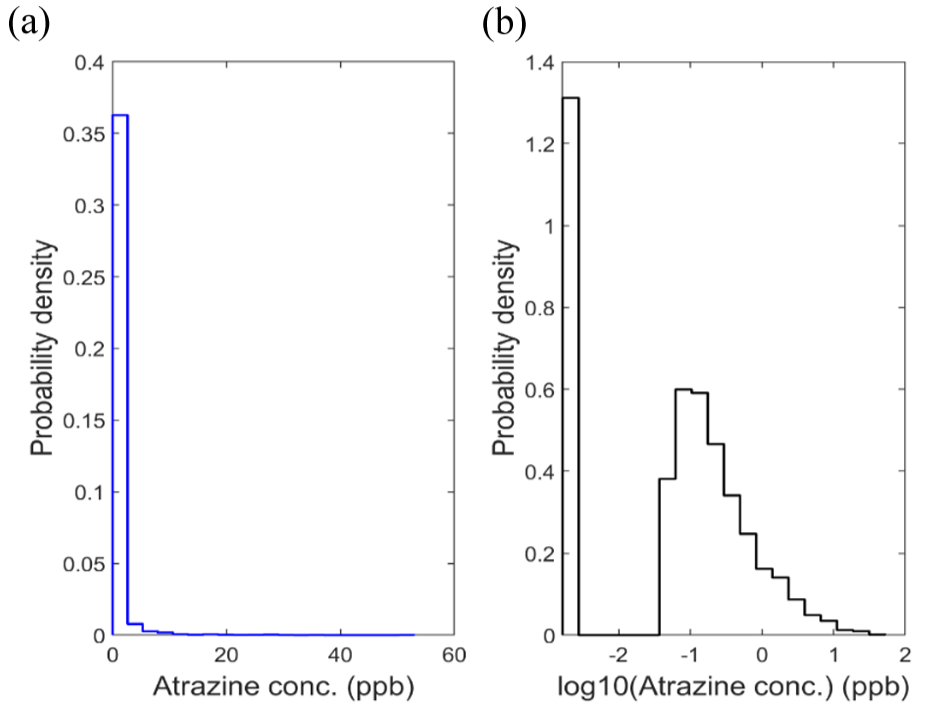
Probability density distribution of raw atrazine concentration, µg/L (a) and log-transformed concentration (b) data.

After log₁₀ transformation, the distribution approximates normality (Figure 3b), centering around −1 log units (~0.1 µg/L). This transformation reduced skewness, stabilized variance, and aligned the data with the Gaussian assumptions required for covariance modeling in the spatiotemporal analysis. The heavy-tailed raw distribution underscores the episodic nature of atrazine contamination, where infrequent but extreme runoff events disproportionately influence exposure. As stated previously in the methods all references to log refer to log₁₀, however, unless noted, all results are shown in the µg/L, non-transformed values.

The temporal trends of observed atrazine concentrations from 2000 to 2004 reveal strong seasonal patterns, with sharp peaks each spring and early summer likely coinciding with herbicide application and subsequent runoff events (Figure 4, left). These pulses typically exceed background levels by an order of magnitude and persist for several weeks, seemingly consistent with atrazine’s environmental half-life and hydrological transport. The temporal structure supports the fitted covariance model shown in Figure 5, which estimated a temporal correlation range of ~50 days, indicating concentrations remain significantly autocorrelated across 2-month periods.

Figure 4.

Temporal dynamics and covariance structure of atrazine concentrations (µg/L) in Iowa surface waters (2000–2004).

Figure 5.

Leave-one-out cross-validation results for the spatiotemporal covariance model.

The fitted spatial covariance model (Figure 4, right top) displays a sill of 0.8 and a spatial range with a sharp drop off after ~25 km, and minimal little correlation after 150 km. The sill represents the variance explained by spatial structure. The range represents the distance at which the exponential covariance function decays to approximately 5% of its initial value, marking the practical limit of spatial/temporal dependence between monitoring sites. The fitted temporal covariance model (Figure 4, right, bottom) exhibited a sharp decline within the first 20 days, with minimal temporal dependence beyond approximately 50 days.

Leave-one-out cross-validation (LOOCV) statistics were computed to evaluate the predictive performance of both the traditional spatial-only model and the spatiotemporal model for atrazine concentrations in stream water. Results are summarized in Table 2. Across all error metrics, the spatiotemporal model outperformed the spatial-only model. Prediction bias was reduced, with mean error shifting closer to zero. Specifically, the advanced model reduced overall estimation error (MSE = 0.318 vs. 0.432, 26.4% reduction) and root mean square error (RMSE = 0.564 vs. 0.657, 14.2% reduction), while also increasing explained variance (R² = .73 vs. .64, 14% improvement). The mean absolute error (MAE) was also slightly lower in the spatiotemporal model (0.387 vs. 0.412, 6.1% reduction), indicating more consistent predictions across the range of observed concentrations. Incorporating temporal autocorrelation substantially improved predictive performance. Most predictions are reasonably accurate producing a low MAE in both models. Episodic high-concentration events disproportionately influence MSE, and incorporating temporal autocorrelation reduced these large errors, improving prediction stability and reliability during high-application periods.

Table 2.

Leave-One-Out Cross-Validation Statistics for Atrazine Concentration Estimation in Stream Water Using BME with Traditional Geostatistics (Spatial Covariance) and Advanced Geostatistics (Spatiotemporal Covariance) Models.

Model type	MSE (log– µg/L)²	RMSE (log– µg/L)	MAE (log–µg/L)	ME (log–µg/L)	R² (unitless)
Spatial covariance	0.432	0.657	0.412	0.009	.641
Spatiotemporal covariance	0.318	0.564	0.387	−0.006	.731
Percent improvement in prediction	26.4%	14.2%	6.1%	−33%	14%

The spatiotemporal framework not only captures geographic similarity among neighboring sites but also leverages the strong temporal structure identified in the covariance analysis. Importantly, the 14-point increase in R² demonstrates spatiotemporal autocorrelation explains a substantial portion of the variation in atrazine concentrations spatial models alone fail to capture. The cross-validation scatterplot (Figure 5) further illustrates this improvement. The spatiotemporal predictions exhibit general alignment with the 1:1 line across much of the concentration range and low systematic deviation at higher concentrations.

Figure 6 compares spatial and spatiotemporal BME model outputs for two representative months, May 2003 and June 2004. The spatial-only models (Figures 6a and b) capture broad east–west gradients in atrazine concentrations, with consistently elevated values in eastern Iowa. However, these maps smooth over local variability, muting sharp contamination peaks. By contrast, the spatiotemporal models (Figures 6c and d) incorporate both spatial proximity and temporal persistence, producing more detailed and dynamic contamination patterns. Predicted concentrations are notably higher and more spatially differentiated in eastern and southeastern Iowa. This effect is especially evident along downstream reaches, where temporal autocorrelation reinforces spatial connectivity within watersheds.

Figure 6.

(a) Space- only BME map of atrazine concentrations, May 2003. Predictions reflect broad regional patterns but smooth over localized hotspots. (b) Space-only BME map of atrazine concentrations, June 2004. Elevated values appear across the east, but temporal persistence is not incorporated. (c) Space-time BME map of atrazine concentrations, May 2003. Incorporating temporal correlation reveals sharper contamination hotspots in eastern Iowa. (d) Space-time BME map of atrazine concentrations, June 2004. Predictions capture both regional gradients and persistent contamination aligned with spring runoff and application timing.

In May 2003, the spatiotemporal model captures pronounced hotspots in eastern watersheds following spring applications, features the spatial-only model underestimates. The greater divergence between models during this month may reflect early-season variability and rapid temporal changes, conditions under which temporal correlation provides critical context and stabilizes predictions from sparse observations. By June 2004, when atrazine concentrations had likely stabilized after application and runoff, both models converge toward similar spatial patterns. This convergence suggests temporal autocorrelation contributes most strongly during periods of rapid change and episodic transport, while spatial structure dominates once concentrations equilibrate.

Discussion

Our findings show atrazine contamination in Iowa is structured by both spatial proximity and temporal persistence. Seasonal runoff and slow degradation likely could drive strong temporal autocorrelation, which the spatial-only model struggles to capture. Atrazine’s spatial covariance show concentrations remain correlated across very large domains, far exceeding the scale of individual fields. This pattern suggests contamination is not purely local and may reflect regional-scale application practices and river network connectivity. Such broad correlation appears consistent with widespread atrazine use across the Corn Belt and hydrological transport through connected waterways (U.S. Geological Survey, 2025b). The temporal covariance results indicate elevated atrazine levels persist for nearly 2-month intervals, likely reflecting both the herbicide’s persistence in aquatic systems and the timing of spring applications. Furthermore, the temporal range aligns with atrazine’s environmental half-life and with runoff pulses following major rainfall events. This temporal structure demonstrates contamination events are likely not isolated spikes but instead create lingering signals shaping concentration dynamics for extended periods.

Together, the spatial and temporal covariance functions demonstrate atrazine contamination in Iowa’s stream network is structured, predictable, and driven by regional-scale agricultural and hydrological processes. However, the estimated spatial and temporal covariance parameters reflect statistical dependence in observed atrazine concentrations rather than direct measurements of physical transport, degradation, or hydrological processes. The irregular spacing of monitoring sites and uneven sampling intensity further highlight the need for geostatistical approaches capable of interpolating across unsampled areas and times.

Future research could focus on integrating BME with mechanistic models and remote sensing data, leveraging its modeled data framework to incorporate hydrological and process-based information, and expanding BME’s application to real-time pesticide surveillance through IoT-enabled networks. While fate-and-transport models are resource-intensive, require pollutant-specific parameters, laboratory calibration, dense sampling, and can overestimate degradation of atrazine in soils (Chavez Rodriguez et al., 2021), they can provide complementary strengths to a BME model. They explicitly simulate chemical degradation pathways, hydrological fluxes, and pollutant-specific processes in ways that BME cannot. As a result, mechanistic models are better suited for scenario testing and causal inference under changing conditions (e.g. altered rainfall, soil properties, or crop rotations). Whereas BME excels at interpolating observed data across sparse monitoring networks and can be applied anywhere regardless of geographic location. Furthermore, the BME framework has the flexibility to incorporate and analyze multiple data and modeling structures sources within one framework. Future work could therefore evaluate whether incorporating mechanistic model outputs into BME improves prediction accuracy, and conversely whether BME can help refine mechanistic modeling by identifying persistent spatiotemporal structures in observed contamination patterns.

The largest performance gains associated with the spatiotemporal model occurred in metrics sensitive to extreme errors, particularly MSE. This pattern likely reflects the episodic nature of atrazine transport, where high-concentration events could be driven by application timing and rainfall dominate overall variability. Spatial-only models may tend to smooth these peaks, leading to occasional but substantial prediction errors. These results underscore the importance of explicitly modeling temporal dependence when predicting agrichemical exposures characterized by event-driven dynamics. Temporal autocorrelation appears to contribute most strongly during periods of rapid change and episodic transport, while spatial structure dominates once concentrations stabilize, resulting in reduced large prediction errors and improved overall predictive stability. As a retrospective interpolation, temporally adjacent observations were retained in cross-validation. Consequently, these standardized geostatistical performance metrics reflect the model’s ability to reconstruct observed spatiotemporal patterns given the full monitoring context, rather than to predict future concentrations in the absence of nearby temporal information.

While this study emphasizes comparative predictive performance between spatial and spatiotemporal models, we do not explicitly quantify prediction uncertainty or spatial variability in confidence across the study domain. As with all geostatistical estimates derived from irregular monitoring networks, uncertainty is expected to vary spatially, with higher confidence in regions of denser sampling and lower confidence in sparsely monitored areas. Consequently, predicted atrazine concentrations should be interpreted as best estimates given available data rather than precise exposure values at individual locations. Future work could extend this framework by explicitly mapping prediction uncertainty and incorporating uncertainty-aware exposure metrics to better support regulatory and policy applications.

In addition to uncertainty considerations, this study models spatial dependence using Euclidean distance and does not explicitly incorporate stream network connectivity or watershed flow structure. While flow-connected geostatistical frameworks may improve physical interpretability of in-stream transport processes, they also require substantially more detailed hydrological data and impose additional modeling complexity that is not always feasible at statewide scales. Euclidean distance–based approaches remain appropriate for capturing regional-scale patterns driven by synchronized application timing, precipitation events, and shared climatic forcing, which strongly influence atrazine transport and persistence. Future work could explicitly examine the relative contributions of Euclidean proximity versus flow-connected structure in explaining water quality variability under network-based and Euclidean spatiotemporal frameworks.

National pesticide monitoring programs have contracted substantially since the early 2000s, limiting the availability of high-resolution, long-term water quality data. In this context, spatiotemporal modeling offers a flexible framework for analyzing exposure patterns, identifying periods and locations of elevated risk, and supporting large-scale water quality assessment and future monitoring strategies. This framework can easily be extended to other persistent agricultural contaminants (Jat & Serre, 2016, 2018; Reyes & Serre, 2014). However, this study relies on atrazine concentration data collected between 2000 and 2004, and results should be interpreted in light of potential changes in agricultural practices, regulatory frameworks, and climatic conditions since that period. Although atrazine application rates across the U.S. Corn Belt have remained relatively stable over time, this study does not assume concentration levels or exposure patterns directly reflect present-day conditions.

This study is limited in several ways. First, the analysis is restricted to 4 years of data (2000–2004) and to one state (Iowa), which constrains the generalizability of findings to other regions or time periods. Second, the dataset relies exclusively on publicly available monitoring records, which are irregularly spaced across sites and uneven in temporal coverage. As a result, the findings are not nationally representative but highlight the enduring value of historical monitoring when paired with advanced modeling. While BME provides clear advantages over spatial-only approaches, its implementation, particularly at massive scales, still demands computational resources, specialized statistical expertise and custom analytical workflows.

Conclusions

By extending the value of historical data through spatiotemporal modeling, this study provides tools to improve pesticide monitoring and inform water resource protection (L. Fox et al., 2023; Xu et al., 2016). It represents one of the few systematic, state-level assessments of atrazine contamination using modern spatiotemporal methods and offers methodological advances with enduring relevance (Jat & Serre, 2018; Messier et al., 2015). National monitoring programs have contracted sharply since the early 2000s, the U.S. Geological Survey’s NAWQA program ended in 2001, and the USDA’s Agricultural Chemical Use Program ceased regular reporting in 2021 (U.S. Department of Agriculture, National Agricultural Statistics Service, 2022; U.S. Geological Survey, 2025b). Despite this decline in surveillance, atrazine remains one of the most heavily applied herbicides in U.S. agriculture, with application rates stable at 60 to 80 million pounds annually across the Corn Belt. Iowa and neighboring Midwestern states continue to represent the nation’s highest-use areas (U.S. Environmental Protection Agency, 2025; Sass & Colangelo, 2006), reinforcing the relevance of our historical dataset to present-day conditions. In the absence of renewed national monitoring, spatiotemporal geostatistical modeling provides a practical and scalable pathway for tracking pesticide exposure risks.

Footnotes

Acknowledgements

The authors thank the Iowa Department of Natural Resources for making surface water monitoring data publicly available. The interpretations and conclusions presented here are those of the authors and do not necessarily reflect the views of the data providers.

ORCID iDs

Lani Fox

Sudhansu Panda

Ethical Considerations

This study involved analysis of publicly available environmental monitoring data and did not involve interaction with human subjects or access to identifiable personal information; therefore, ethical approval was not required.

Author Contributions

Prahlad Jat led the data analysis and geostatistical modeling and contributed to manuscript drafting and editing. Lani Fox led manuscript development, including primary drafting, substantive editing, methodological framing, additional analysis, and interpretation of results, and provided direction on analytical refinements. Sudhansu S. Panda contributed to manuscript editing and critical revision. All authors made substantial contributions to the study design, data collection or analysis, drafted or critically revised the article. All have approved the final version of this manuscript, and agree to be accountable for all aspects of the work.

Funding

The authors received no financial support for the research, authorship, and/or publication of this article.

Declaration of Conflicting Interests

The authors declared no potential conflicts of interest with respect to the research, authorship, and/or publication of this article.

Data Availability Statement

All data used in this study are publicly available from the Iowa Department of Natural Resources and the University of Iowa Water Quality Monitoring Program.

References

Abbott

N. A.

Semone

Strott

(2025). Evaluation of Bayesian maximum entropy data fusion approaches to estimate VOCs in the US Gulf states. Environmental Science & Technology, 59, 45–55. https://doi.org/10.1021/acs.est.4c05094

Agency for Toxic Substances and Disease Registry. (2025). Toxicological profile for atrazine (Publication No. TP153). U.S. Department of Health and Human Services. https://www.atsdr.cdc.gov/toxprofiles/tp153-c1-b.pdf

Bogaert

Christakos

Jerrett

H. L.

(2009). Spatiotemporal modelling of ozone distribution in the State of California. Atmospheric Environment, 43, 2471–2480. https://doi.org/10.1016/j.atmosenv.2009.01.049

Center for Biological Diversity. (2025). Atrazine preliminary ecological risk assessment. https://www.biologicaldiversity.org/campaigns/pesticides_reduction/pdfs/AtrazinePreliminaryERA.pdf

Chavez Rodriguez

Ingalls

Meierdierks

Kundu

Streck

Pagel

. (2021). Modeling bioavailability limitations of atrazine degradation in soils. Frontiers in Environmental Science, 9, 706457. https://doi.org/10.3389/fenvs.2021.706457

Christakos

(1990). A Bayesian/maximum-entropy view to the spatial estimation problem. Mathematical Geology, 22, 763–777. https://doi.org/10.1007/bf00890661

Christakos

(1998). Spatiotemporal information systems in soil and environmental sciences. Geoderma, 85, 141–179. https://doi.org/10.1016/s0016-7061(98)00018-4

Christakos

Bogaert

Serre

M. L.

(2001). Knowledge base synthesis. In Temporal GIS: Advanced functions for field-based applications (pp. 33–52). Springer.

Christakos

Serre

M. L.

(2000). Spatiotemporal analysis of environmental exposure–health effect associations. Journal of Exposure Science & Environmental Epidemiology, 10, 168–187. https://doi.org/10.1038/sj.jea.7500077

10.

Cliff

Ord

(1981). Spatial processes: Models and applications. Pion. https://archive.org/details/spatialprocesses0000clif/page/n5/mode/2up

11.

Delhomme

J. P.

(1978). Kriging in the hydro sciences. Advances in Water Resources, 1(5), 251–266. https://doi.org/10.1016/0309-1708(78)90039-8

12.

de Nazelle

Arunachalam

Serre

M. L

. (2010). Bayesian maximum entropy integration of ozone observations and model predictions. Environmental Science & Technology, 44, 5707–5713. https://doi.org/10.1021/es100228w

13.

Fox

L. C.

Miller

W. C.

Gesink

Doherty

Hampton

K. H.

Leone

P. A.

Williams

D. E.

Akita

Dunn

Serre

M. L.

(2023). Progression of a large syphilis outbreak in rural North Carolina through space and time: Application of a Bayesian maximum entropy graphical user interface. PLOS Global Public Health, 3, e0001714. https://doi.org/10.1371/journal.pgph.0001714

14.

Fox

Miller

W. C.

Gesink

Doherty

Serre

(2024). Enhancing insights in sexually transmitted infection mapping: Syphilis in Forsyth County, North Carolina, a case study. Plos Computational Biology, 20, e1012464. https://doi.org/10.1371/journal.pcbi.1012464

15.

Fox

Peter

B. G.

Frake

A. N.

Messina

J. P.

(2023). A Bayesian maximum entropy model for predicting Tsetse ecological distributions. International Journal of Health Geographics, 22, 31. https://doi.org/10.1186/s12942-023-00349-0

16.

Fox

Serre

M. L.

Lippmann

S. J.

Rodríguez

D. A.

Bangdiwala

S. I.

Gutiérrez

M. I.

Escobar

Villaveces

(2015). Spatiotemporal approaches to analyzing pedestrian fatalities: The case of Cali, Colombia. Traffic Injury Prevention, 16, 571–577. https://doi.org/10.1080/15389588.2014.976336

17.

Christakos

(2023). Bayesian maximum entropy. In Encyclopedia of mathematical geosciences. Springer.

18.

Iowa Department of Natural Resources. (2025). Ambient stream monitoring program. https://www.iowadnr.gov/environmental-protection/water-quality/water-quality-monitoring-assessment/ambient-stream-monitoring

19.

Isaak

D. J.

Peterson

E. E.

Ver Hoef

J. M.

Wenger

S. J.

Falke

J. A.

Torgersen

C. E.

Sowder

Steel

E. A.

Fortin

Jordan

C. E.

Ruesch

A. S.

Som

Monestiez

(2014). Applications of spatial statistical network models to stream data. WIREs Water, 1(3), 277–294. https://doi.org/10.1002/wat2.1023

20.

Isaaks

E. H.

Srivastava

R. M.

(1989). Applied geostatistics. Oxford University Press.

21.

Jat

Serre

M. L.

(2016). Bayesian maximum entropy space/time estimation of surface water chloride in Maryland using river distances. Environmental Pollution, 219, 1148–1155. https://doi.org/10.1016/j.envpol.2016.09.020

22.

Jat

Serre

M. L.

(2018). A novel geostatistical approach combining Euclidean and gradual-flow covariance models to estimate fecal coliform along the haw and deep rivers in North Carolina. Stochastic Environmental Research and Risk Assessment, 32, 2537–2549. https://doi.org/10.1007/s00477-018-1512-6

23.

Lerro

C. C.

Beane Freeman

L. E.

Portengen

Kang

Lee

Blair

Lynch

C. F.

Bakke

De Roos

A. J.

Vermeulen

R. C.

(2017). A longitudinal study of atrazine and 2,4-D exposure and oxidative stress markers among Iowa corn farmers. Environmental and Molecular Mutagenesis, 58(1), 30–38. https://doi.org/10.1002/em.22069

24.

LoBuglio

J. N.

Characklis

G. W.

Serre

M. L.

(2007). Cost-effective water quality assessment through the integration of monitoring data and modeling results. Water Resources Research, 43(3), W03419. https://doi.org/10.1029/2006wr005020

25.

MathWorks. (2022). MATLAB R2022b (Version 9.0) [Computer software]. The MathWorks, Inc. https://www.mathworks.com/products/matlab.html

26.

Messier

K. P.

Akita

Serre

M. L.

(2012). Integrating address geocoding, land use regression, and spatiotemporal geostatistical estimation for groundwater tetrachloroethylene. Environmental Science & Technology, 46, 2772–2780. https://doi.org/10.1021/es203152a

27.

Messier

K. P.

Campbell

Bradley

P. J.

Serre

M. L.

(2015). Estimation of groundwater radon in North Carolina using land use regression and Bayesian maximum entropy. Environmental Science & Technology, 49(16), 9817–9825. https://doi.org/10.1021/acs.est.5b01503

28.

Peterson

E. E.

Urquhart

N. S.

(2006). Predicting water quality impaired stream segments using landscape-scale data and a regional geostatistical model: A case study in Maryland. Environmental Monitoring and Assessment, 121, 615–638. https://doi.org/10.1007/s10661-005-9163-8

29.

Reyes

J. M.

Serre

M. L.

(2014). An LUR/BME framework to estimate PM2.5 explained by on road mobile and stationary sources. Environmental Science & Technology, 48, 1736–1744. https://doi.org/10.1021/es403870f

30.

Roh

Knappett

P. S. K.

Han

Ludewig

Kelly

K. M.

Wang

Weyer

P. J.

(2023). Characterization of arsenic and atrazine contaminations in drinking water in Iowa: A public health concern. International Journal of Environmental Research and Public Health, 20(7), 5397. https://doi.org/10.3390/ijerph20075397

31.

Sass

J. B.

Colangelo

(2006). European Union bans atrazine while the United States negotiates continued use. International Journal of Occupational and Environmental Health, 12, 260–267. https://doi.org/10.1179/oeh.2006.12.3.260

32.

Serre

M. L.

(2022). The UNC BMELab: BMELib and BMEGUI. https://mserre.sph.unc.edu/BMElab_web/

33.

Serre

M. L.

Christakos

(1999). Modern geostatistics: Computational BME analysis in the light of uncertain physical knowledge - the Equus beds study. Stochastic Environmental Research and Risk Assessment, 13(1-2), 1–26. https://doi.org/10.1007/s004770050029

34.

U.S. Department of Agriculture, National Agricultural Statistics Service. (2022). 2021 agricultural chemical use survey: Corn. https://www.nass.usda.gov/Surveys/Guide_to_NASS_Surveys/Chemical_Use/2021_Field_Crops/chemhighlights-corn.pdf

35.

U.S. Environmental Protection Agency. (2025). Atrazine. https://www.epa.gov/ingredients-used-pesticide-products/atrazine

36.

U.S. Geological Survey. (2025a). National hydrography dataset (NHD). http://nhd.usgs.gov/

37.

U.S. Geological Survey. (2025b). Pesticide national synthesis project—Atrazine. https://water.usgs.gov/nawqa/pnsp/usage/maps/show_map.php?year=2019↦=ATRAZINE&hilo=L&disp=Atrazine

38.

Valencia

Serre

Arunachalam

(2023). A hyperlocal hybrid data fusion near-road PM2.5 and NO₂ annual risk and environmental justice assessment across the United States. PLoS One, 18, e0286406. https://doi.org/10.1371/journal.pone.0286406

39.

Serre

M. L.

Reyes

Vizuete

(2016). Bayesian maximum entropy integration of ozone observations and model predictions: A national application. Environmental Science & Technology, 50, 4393–4400. https://doi.org/10.1021/acs.est.6b00096

Enriching Agricultural Pesticide Modeling in Surface Waters Through Integrated Space–Time Geostatistics: Atrazine in Iowa,A Case Study

Abstract

Keywords

Background

Methods

Data

Analysis Strategy

Results

Discussion

Conclusions

Footnotes

Acknowledgements

ORCID iDs

Ethical Considerations

Author Contributions

Funding

Declaration of Conflicting Interests

Data Availability Statement

References